matlab有限元并行计算
- 格式:pdf
- 大小:943.96 KB
- 文档页数:5
Matlab技术算法并行化与加速技巧引言Matlab作为一种高级技术计算软件,旨在为科学家和工程师提供一种快速、简单的实现数值计算算法的环境。
然而,随着问题规模和计算复杂度的增加,单线程的执行往往无法满足现代计算的需求。
本文将探讨如何利用Matlab提供的并行化和加速技巧,优化算法的性能和效率。
一、并行计算基础并行计算是一种将计算任务分解为独立子任务,同时执行并合并结果的计算方法。
在Matlab中,可以通过使用并行计算工具箱中的函数和特性来实现算法的并行化。
1. 启用并行计算在Matlab中,可以通过Parallel Computing Toolbox来启用并行计算功能。
使用parpool函数可以创建一个并行池,用于执行并行任务。
例如:```matlabparpool('local', 4);```上述代码将创建一个具有4个工作进程的本地并行池。
可以根据计算机的处理器核心数和内存容量来选择合适数量的工作进程。
2. 并行循环Matlab提供了parfor循环,用于并行执行迭代计算。
该循环会将每个迭代的计算任务分配给不同的工作进程,并在所有工作进程完成后合并结果。
以下是一个简单的parfor示例:parfor i=1:n% 并行计算任务end```需要注意的是,由于并行计算涉及多个工作进程之间的数据共享,因此必须谨慎处理循环内的变量和数据依赖关系。
可以使用spmd结构来实现更复杂的并行计算任务。
二、加速技巧除了并行计算之外,Matlab还提供了一些其他的加速技巧,可以显著提高算法的执行速度和效率。
1. 向量化运算向量化是一种通过使用矩阵和数组运算来替代循环和逐元素计算的技术。
在Matlab中,向量化可以大大提高算法的性能,因为矩阵和数组运算通常由底层的高度优化的计算库执行。
例如,考虑以下代码片段:```matlabfor i=1:numel(a)b(i) = a(i) + 1;end```可以使用向量化来替代循环,如下所示:b = a + 1;```向量化不仅可以提高计算速度,还可以使代码更简洁和易读。
Matlab并行计算工具箱及MDCE介绍.doc3.1 Matlab并行计算发展简介MATLAB技术语言和开发环境应用于各个不同的领域,如图像和信号处理、控制系统、财务建模和计算生物学。
MATLAB通过专业领域特定的插件(add-ons)提供专业例程即工具箱(Toolbox),并为高性能库(Libraries)如BLAS(Basic Linear Algebra Subprograms,用于执行基本向量和矩阵操作的标准构造块的标准程序)、FFTW(Fast Fourier Transform in the West,快速傅里叶变换)和LAPACK(Linear Algebra PACKage,线性代数程序包)提供简洁的用户界面,这些特点吸引了各领域专家,与使用低层语言如C语言相比可以使他们很快从各个不同方案反复设计到达功能设计。
计算机处理能力的进步使得利用多个处理器变得容易,无论是多核处理器,商业机群或两者的结合,这就为像MATLAB一样的桌面应用软件寻找理论机制开发这样的构架创造了需求。
已经有一些试图生产基于MATLAB的并行编程的产品,其中最有名是麻省理工大学林肯实验室(MIT Lincoln Laboratory)的pMATLAB和MatlabMPI,康耐尔大学(Cornell University)的MutiMATLAB和俄亥俄超级计算中心(Ohio Supercomputing Center)的bcMPI。
MALAB初期版本就试图开发并行计算,80年代晚期MATLAB的原作者,MathWorks公司的共同创立者Cleve Moler曾亲自为英特尔HyperCube和Ardent 电脑公司的Titan超级计算机开发过MATLAB。
Moler 1995年的一篇文章“Why there isn't a parallel MATLAB?[**]” 中描述了在开了并行MATLAB语言中有三个主要的障碍即:内存模式、计算粒度和市场形势。
Matlab并行计算技术的应用指南1. 引言在现代科学和工程领域中,计算机模拟和数据处理已经成为不可或缺的工具。
而在这个过程中,高性能计算成为了关键。
Matlab作为一种功能强大的科学计算软件,在处理大规模数据和计算复杂模型时发挥着重要作用。
而并行计算技术的应用可以帮助Matlab进一步提升计算效率,加速模拟和数据分析的速度。
本文将介绍Matlab并行计算技术的应用指南,帮助读者更好地利用这种技术提升计算效率。
2. 并行计算的基础知识在了解如何应用Matlab并行计算技术之前,我们先来了解一些并行计算的基础知识。
并行计算是一种利用多个处理单元(例如多个CPU或GPU)同时进行计算的技术。
这样做可以将一个计算任务划分成多个子任务,分配到不同的处理单元上进行并行计算,从而加速计算过程。
常见的并行计算技术包括向量化计算、多线程计算和分布式计算等。
3. Matlab中的并行计算工具Matlab提供了多种并行计算工具,用于实现并行计算。
其中最常用的有Parallel Computing Toolbox和Distributed Computing Server。
3.1 Parallel Computing ToolboxParallel Computing Toolbox是Matlab中用于实现并行计算的工具箱。
它提供了函数和工具,用于将计算任务分解为独立的子任务,并将其分配到多个处理单元上并行计算。
通过使用Parallel Computing Toolbox,可以充分利用多核处理器和集群计算资源,提升Matlab的计算效率。
3.2 Distributed Computing ServerDistributed Computing Server是Matlab中的一个可选工具,用于进行分布式计算。
分布式计算是一种将计算任务分配到多个机器上进行并行计算的技术。
通过使用Distributed Computing Server,可以将Matlab计算任务分布到远程机器或者云服务上进行计算,从而进一步提升计算效率。

快速入门Matlab并行计算的基本步骤引言:在当前高速发展的科技时代,计算速度的提升变得尤为重要。
为解决复杂问题,Matlab提供了并行计算的功能,可以有效提高计算效率。
本文将介绍快速入门Matlab并行计算的基本步骤,帮助读者更好地掌握该技术。
一、并行计算简介首先,我们来了解并行计算的基本概念。
并行计算是指同时运行多个计算任务,通过资源共享和任务划分,加快计算速度。
这种方式可以充分利用多核处理器、集群计算等硬件设备,提高计算效率。
二、Matlab并行计算的优势Matlab具备并行计算功能,其并行计算工具箱提供了一系列函数和工具,使用户能够充分利用计算机的多核处理能力,提高计算速度。
相比传统的串行计算,Matlab并行计算具有如下优势:1. 节省时间:通过并行计算,可以同时处理多个计算任务,缩短计算时间。
2. 提高效率:充分利用计算机资源,提高计算效率,减少等待时间。
3. 扩展性好:支持任务的拆分和分发,适用于大规模的计算。
三、准备工作在使用Matlab进行并行计算之前,需要进行一些准备工作。
下面列出了几个关键步骤:1. 安装并配置并行计算工具箱:确保已经安装并行计算工具箱,并按照官方文档进行配置。
2. 编写并行代码:根据实际需求,编写并行计算的代码,并注意代码的正确性和可调试性。
3. 准备数据:根据需要,准备好待处理的数据,并组织好数据的结构。
四、使用并行计算工具箱在准备工作完成后,我们可以开始使用Matlab提供的并行计算工具箱。
以下是一些基本的步骤和注意事项:1. 初始化并行环境:在代码的开始处,使用parpool函数初始化并行环境。
例如:```matlabparpool();```2. 并行循环:对于可并行化的任务,可以使用parfor函数实现并行化的循环。
例如,在计算一个向量的平方和时,可以使用以下方式:```matlabn = 1000;data = rand(1,n);result = 0;parfor i = 1:nresult = result + data(i)^2;end```3. 并行函数:除了循环,Matlab还提供了其他的并行计算函数,如spmd、parfeval等,可以根据具体情况选择使用。
Getting Started with Parallel Computing usingMATLAB: Interactive and Scheduled ApplicationsCreated by S. Zaranek, E. Johnson and A. Chakravarti1.ObjectivesThis user guide provides an end user with instructions on how to get started running parallel MATLAB applications using a desktop computer or a cluster.2.AssumptionsUser has access to MATLAB and Parallel Computing Toolbox on the desktopcomputer or head node of the cluster.If running on a cluster:MATLAB Distributed Computing Server has been installed by an administrator on the cluster.The desktop MATLAB client has been configured to connect to the cluster. If this hasnot been done, you should contact the cluster administrator.3. Getting the Example FilesUnzip the demoFiles.zip file that was provided along with this guide. You can add the files to the MATLAB path by running the addpath command in MATLAB.>> addpath <location of files>4. Examples Running LocallyIn this section, you will be running and submitting jobs using the localconfiguration.If your workflow will ultimately involve submitting jobs to a cluster, you canfollow this section by switching the default configuration from local to that ofyour cluster and running these jobs again. This is described in Section 5.You can set the configuration to local, either at the command-line>> defaultParallelConfig('local')or by using the user interface found in the parallel menu. See screen snapshot below.For more information on configurations and programming with user configurations, see:/access/helpdesk/help/toolbox/distcomp/index.html?/a ccess/helpdesk/help/toolbox/distcomp/f5-16141.html#f5-165401. Using an Interactive MATLAB poolTo interactively run your parallel code, you first need to open a MATLAB pool. This reserves a collection of MATLAB worker sessions to run your code. The MATLAB pool can consist of MATLAB sessions running on your local machine or on a remote cluster. In this case, we are initially running on your local machine. You can use matlabpool open to start an interactive worker pool. If the number of workers is not defined, the default number defined in your configuration will be used. A good rule of thumb is to not open more workers then cores available. If the Configuration argument is not provided, matlabpool will use the default configuration as setup in the beginning of this section. When you are finished running with your MATLAB pool, you can close it using matlabpool close. Two of the main parallel constructs that can be run on a MATLAB pool are parfor loops (parallel for-loops) and spmd blocks (single program - multiple data blocks). Both constructs allow for a straight-forward mixture of serial and parallel code.parfor loops are used for task-parallel (i.e. embarrassingly parallel) applications. parfor is used to speed up your code. Below is a simple for loop converted into a parfor to run in parallel, with different iterations of the loop running ondifferent workers. The code outside the parfor loop executes as traditional MATLAB code (serially, in your client MATLAB session).Note: The example below is located in the m-file, ‘parforExample1.m’.matlabpool open2% can adjust according to your resourcesN = 100;M = 200;a = zeros(N,1);tic; % serial (regular) for-loopfor i = 1:Na(i) = a(i) + max(eig(rand(M)));endtoc;tic; % parallel for-loopparfor i = 1:Na(i) = a(i) + max(eig(rand(M)));endtoc;matlabpool closespmd blocks are a single program multiple data (SPMD) language construct. The "single program" aspect of spmd means that the identical code runs on multiple labs. The code within the spmd body executes simultaneously on the MATLAB workers. The "multiple data" aspect means that even though the spmd statement runs identical code on all workers, each worker can have different, unique data for that code.spmd blocks are useful when dealing with large data that cannot fit on a single machine. Unlike parfor, spmd blocks support inter-worker communication. They allow:Arrays (and operations on them) to be distributed across multiple workersMessages to be explicitly passed amongst workers.The example below creates a distributed array (different parts of the array arelocated on different workers) and computes the svd of this distributed array. The spmd block returns the data in the form of a composite object (behaves similarly to cells in serial MATLAB. For specifics, see the documentation link below).Note: The example below is located in the m-file, ‘spmdExample1.m’.matlabpool open2% can adjust according to your resourcesM = 200;spmdN = rand(M,M,codistributor); % 200x100 chunk per workerA = svd(N);endA = max(A{1}); % Indexing into the composite objectdisp(A)clear Nmatlabpool closeFor information on matlabpool, see:/access/helpdesk/help/toolbox/distcomp/index.html?/a ccess/helpdesk/help/toolbox/distcomp/matlabpool.htmlFor information about getting started using parfor loops, see:/access/helpdesk/help/toolbox/distcomp/index.html?/a ccess/helpdesk/help/toolbox/distcomp/brb2x2l-1.htmlFor information about getting started using spmd blocks, see:/access/helpdesk/help/toolbox/distcomp/index.html?/a ccess/helpdesk/help/toolbox/distcomp/brukbno-2.htmlFor information regarding composite objects:/access/helpdesk/help/toolbox/distcomp/index.html?/a ccess/helpdesk/help/toolbox/distcomp/brukctb-1.htmlFor information regarding distributed arrays:/access/helpdesk/help/toolbox/distcomp/index.html?/a ccess/helpdesk/help/toolbox/distcomp/bqi9fln-1.html2a. Using Batch to Submit Serial Code (Best for Scripts)batch sends your serial scriptto run on one worker in yourcluster. All of the variables inyour client workspace (e.g. theMATLAB process you aresubmitting from) are sent to the worker by default. You can alternatively pass a subset of these variables by defining the Workspace argument and passing the desired variables in a structure.After your job has finished, you can use the load command to retrieve the results from the worker-workspace back into your client-workspace. In this and all examples following, we use a wait to ensure the job is done before we load back in worker-workspace. This is optional, but you can not load the data from a task or job until that task or job is finished. So, we use wait to block the MATLAB command line until that occurs.If the Configuration argument is not provided, batch will use the default configuration that was set up above.Note: For this example to work, you will need ‘testBatch.m’ on the machine that you are submitting from (i.e. the client machine). This example below is located in the m-file, ‘submitJob2a.m’.%% This script submits a serial script using batchjob2a = batch('testBatch');wait(job2a); % only can load when job is finishedsprintf('Finished Running Job')load(job2a); % loads all variables backsprintf('Loaded Variables into Workspace')% load(job2a, 'A'); % only loads variable Adestroy(job2a) % permanently removes job datasprintf('Test Completed')If you have submitted successfully, you should see the following variables appear in your client workspace:For more information on batch, see:/access/helpdesk/help/toolbox/distcomp/index.html?/a ccess/helpdesk/help/toolbox/distcomp/batch.htmland here:/access/helpdesk/help/toolbox/distcomp/index.html?/a ccess/helpdesk/help/toolbox/distcomp/brjw1e5-1.html#brjw1fx-32b. Using Batch to Submit Scripts that Run Using a MATLAB poolbatch with the 'matlabpool'option sends scripts containing parfor or spmd to run on workers via a MATLAB pool. In this process, one worker behaves like a MATLAB client process that facilitates the distribution of the job amongst the workers in the pool and runs the serial portion of the script. Therefore, specifying a 'matlabpool' of size N actually will result in N+1 workers being used.Just like in step 2a, all variables are automatically sent from your client workspace (i.e. the workspace of the MATLAB you are submitting from) to the worker’s workspace on the cluster. load then brings the results from your worker’s workspace back into your client’s workspace. If a configuration is not specified, batch uses the default configuration as defined in the beginning of this section.Note: For this example to work, you will need ‘testParforBatch.m’ on the machine that you are submitting from (i.e. the client machine). This example below is located in the m-file, submitJob2b.m.%% This script submits a parfor script using batchjob2b = batch('testParforBatch','matlabpool',2);wait(job2b); % only can load when job is finishedsprintf('Finished Running Job')load(job2b); % loads all variables backsprintf('Loaded Variables into Workspace')% load(job2b, 'A'); % only loads variable Adestroy(job2b) % permanently removes job datasprintf('Test Completed')If you have submitted successfully, you should see the following variables appear in your client workspace:The above code submitted a script containing a parfor. You can submit a script containing a spmd block in the same fashion by changing the name of the submission script in the batch command.Note: For this example to work, you will need ‘testSpmdBatch.m’ on the machine that you are submitting from (i.e. the client machine). This example below is located in the m-file, submitJob2b_spmd.m.%% This script submits a spmd script using batchjob2b = batch('testSpmdBatch','matlabpool',2);wait(job2b); % only can load when job is finishedsprintf('Finished Running Job')load(job2b); % loads all variables backsprintf('Loaded Variables into Workspace')% load(job2b, 'A'); % only loads variable Adestroy(job2b) % permanently removes job datasprintf('Test Completed')If you have submitted successfully, you should see the following variables appear in your client workspace:3. Run Task-Parallel Example with Jobs and TasksIn this example, we are sending a task parallel job with multiple tasks. Each task evaluates the built-in MATLAB function. The createTask function in the below example is passed the job, the function to be run in the form of a function handle (@sum), the number of output arguments of the function (1), and the input argument to the sum function in the form of a cell array ({[1 1]});If not given a configuration, findResource uses the scheduler found in the default configuration defined in the beginning of this section.Note: This example is located in the m-file, ‘submitJob3a.m’.%% This script submits a job with 3 taskssched = findResource();job3a = createJob(sched);createTask(job3a, @sum, 1, {[1 1]});createTask(job3a, @sum, 1, {[2 2]});createTask(job3a, @sum, 1, {[3 3]});submit(job3a)waitForState(job3a, 'finished') %optionalsprintf('Finished Running Job')results = getAllOutputArguments(job3a);sprintf('Got Output Arguments')destroy(job3a) % permanently removes job datasprintf('Test Completed')If you have submitted successfully, you should see the following variables appear in your client workspace:results should contain the following:You can also call a user-created function in the same way as shown above. In that case, you will need to make sure that any scripts, files, or functions that the task function uses are accessible to the cluster. You can do this by sending those files to the cluster via the FileDependencies property or by directing the worker to a shared directory containing those files via the PathDependencies property. An example of using FileDependencies is shown below:Note: you will need to have a ‘testTask.m’ file on the machine you are submitting from for this example to work. This example is located in the m-file,‘submitJob3b.m’.% This script submits a job with 3 taskssched = findResource();job3b = createJob(sched,'FileDependencies',{'testTask.m'});createTask(job3b, @testTask, 1, {1,1});createTask(job3b, @testTask, 1, {2,2});createTask(job3b, @testTask, 1, {3,3});submit(job3b)waitForState(job3b, 'finished') % optionalsprintf('Finished Running Job')results = getAllOutputArguments(job3b);sprintf('Got Output Arguments')destroy(job3b) % permanently removes job datasprintf('Test Completed')If you have submitted successfully, you should see the following variables appear in your client workspace:results should contain the following:For more information on File and Path Dependencies, see the below documentation.File Dependencies:/access/helpdesk/help/toolbox/distcomp/index.html?/a ccess/helpdesk/help/toolbox/distcomp/filedependencies.htmlPath Dependencies:/access/helpdesk/help/toolbox/distcomp/index.html?/a ccess/helpdesk/help/toolbox/distcomp/pathdependencies.htmlMore general overview about sharing code between client and workers:/access/helpdesk/help/toolbox/distcomp/index.html?/a ccess/helpdesk/help/toolbox/distcomp/bqur7ev-2.html#bqur7ev-94. Run Task-Parallel Example with a MATLAB pool job (best for parfor or spmd in functions)In this example, we are sending a MATLAB pool job with a single task. This is nearly equivalent to sending a batch job (see step 2b) with a parfor or a spmd block, except this method is best used when sending functions and not scripts. It behaves just like jobs/tasks explained in step 3. The function referenced in the task contains a parfor.Note: For this example to work, you will need ‘testParforJob.m’ on the machine that you are submitting from (i.e. the client machine). This example is located in the m-file, ‘submitJob4.m’.% This script submits a function that contains parforsched = findResource();job4 = createMatlabPoolJob(sched,'FileDependencies',...{'testParforJob.m'});createTask(job4, @testParforJob, 1, {});set(job4, 'MaximumNumberOfWorkers', 3);set(job4, 'MinimumNumberOfWorkers', 3);submit(job4)waitForState(job4, 'finished') % optionalsprintf('Finished Running Job')results = getAllOutputArguments(job4);sprintf('Got Output Arguments')sprintf('Test Completed')If you have submitted successfully, you should see the following variables appear in your client workspace:results{1} should contain a [50x1 double].For more information on creating and submitting MATLAB pool jobs, see /access/helpdesk/help/toolbox/distcomp/index.html?/a ccess/helpdesk/help/toolbox/distcomp/creatematlabpooljob.html5. Run Data-Parallel ExampleIn this step, we are sending a data parallel job with a single task. The format is similar to that of jobs/tasks (see step 3). For parallel jobs, you only have one task. That task refers to a function that uses distributed arrays,labindex, or some mpi functionality. In this case, we are running a simple built in function (labindex) which takes no inputs and returns a single output.labindex returns the ID value for each of worker processes that ran the it . The value of labindex spans from 1 to n, where n is the number of labs running the current jobNote: This example is located in the m-file, ‘submitJob5.m’.%% Script submits a data parallel job, with one tasksched = findResource();job5 = createParallelJob(sched);createTask(job5, @labindex, 1, {});set(job5, 'MaximumNumberOfWorkers', 3);set(job5, 'MinimumNumberOfWorkers', 3);submit(job5)waitForState(job5, 'finished') % optionalsprintf('Finished Running Job')results = getAllOutputArguments(job5);sprintf('Got Output Arguments')sprintf('Test Completed')If you have submitted successfully, you should see the following variables appear in your client workspace:results should contain the following:For more information on creating and submitting data parallel jobs, see:/access/helpdesk/help/toolbox/distcomp/index.html?/a ccess/helpdesk/help/toolbox/distcomp/createparalleljob.htmlFor more information on, labindex, see:/access/helpdesk/help/toolbox/distcomp/index.html?/a ccess/helpdesk/help/toolbox/distcomp/labindex.html5 Submitting Jobs to Your ClusterRerun the above section (Section 4) with your configuration changed from local to the configuration name corresponding to your cluster.6. Summary Chart for Scheduling Options✓7. Next StepsRefer to the documentation for the Parallel Computing Toolbox to learn about more functionality for solving your MATLAB problems in parallel. A good place to start is here:/access/helpdesk/help/toolbox/distcomp/index.html?/a ccess/helpdesk/help/toolbox/distcomp/f3-6010.htmlYou can also consider taking a training course through The MathWorks to learnmore in focused, hands-on environment./services/training/index.html。
Matlab的图形处理器并行计算及其在拓扑优化中的应用作者:蔡勇李胜来源:《计算机应用》2016年第03期摘要:针对传统并行计算方法实现结构拓扑优化快速计算的硬件成本高、程序开发效率低的问题,提出了一种基于Matlab和图形处理器(GPU)的双向渐进结构优化(BESO)方法的全流程并行计算策略。
首先,探讨了Matlab编程环境中实现GPU并行计算的三种途径的优缺点和适用范围;其次,分别采用内置函数直接并行的方式实现了拓扑优化算法中向量和稠密矩阵的并行化计算,采用MEX函数调用CUSOLVER库的形式实现了稀疏格式有限元方程组的快速求解,采用并行线程执行(PTX)代码的方式实现了拓扑优化中单元敏度分析等优化决策的并行化计算。
数值算例表明,基于Matlab直接开发GPU并行计算程序不仅编程效率高,而且还可以避免不同编程语言间的计算精度差异,最终使GPU并行程序可以在保持计算结果不变的前提下取得可观的加速比。
关键词:并行计算;图形处理器;拓扑优化;Matlab;有限元分析中图分类号: TP391 文献标志码:A0引言伴随计算机技术和计算技术的快速发展,对大规模数据的处理能力已成为评价各类工程算法的主要准则之一,要求算法具有较强的并行计算能力。
传统的并行计算方法经过多年的发展,已经在多个应用领域内发挥了积极作用,但是,由于其计算平台的计算力与计算核心数直接相关,过多核心数会导致硬件成本过高,限制其在工程实践中的推广应用。
为了降低并行计算的成本,NVIDIA公司根据图形处理器(Graphics Processing Unit, GPU)的可编程性以及其强大的密集数据处理能力,在2006年推出了基于中央处理器(Central Processing Unit,CPU)和GPU异构计算平台的通用并行计算的编程语言和架构,命名为统一计算架构(Compute Unified Device Architecture, CUDA)[1]。
实战matlab并行程序设计MATLAB并行程序设计是一种利用MATLAB的并行计算工具箱来提高计算效率的技术。
在处理大规模数据集或复杂算法时,传统的串行计算方式可能效率低下,而并行程序设计可以显著提升处理速度。
以下是MATLAB并行程序设计的一些关键概念和步骤。
1. 并行计算基础并行计算指的是同时使用多个处理器或核心来执行计算任务。
MATLAB并行程序设计主要依赖于MATLAB的Parallel Computing Toolbox。
2. 环境配置在开始并行程序设计之前,需要确保MATLAB安装了Parallel Computing Toolbox,并且计算机上安装了MATLAB的并行计算服务器。
3. 并行池的创建和管理并行池是执行并行任务的工作单元集合。
MATLAB提供了`parpool`和`delete(gcp('nocreate'))`函数来创建和管理并行池。
```matlab% 创建并行池parpool;% 删除并行池delete(gcp('nocreate'));```4. 并行计算函数MATLAB提供了多种并行计算函数,如`parfor`、`parfeval`、`parfor`等。
`parfor`是最常见的并行循环,用于并行化for循环。
```matlab% 并行for循环parfor i = 1:N% 执行并行任务end```5. 数据分配在并行程序设计中,数据需要在不同的工作单元之间分配。
MATLAB提供了`distribute`函数来帮助实现数据的自动分配。
```matlab% 数据分配data = distribute(largeArray);```6. 并行变量在并行环境中,MATLAB支持两种类型的变量:共享变量和私有变量。
共享变量在所有工作单元中共享,而私有变量则在每个工作单元中独立。
```matlab% 声明共享变量sharedVar = 0;% 声明私有变量parfor i = 1:NlocalVar = rand;end```7. 并行任务的同步在并行程序设计中,有时需要同步不同工作单元的状态。
Matlab 并行计算工具箱的使用Matlab并行工具箱的产生一方面给大规模的数据分析带来了巨大的效益,另一方面且引入了分布式计算,借助matlab自身携带的MDCE,可以实现单机多核并行运行或者是同一个局域网络中的多台处理器组成的机群的并行运行。
个人以为后者是前者的拓展,并行计算的最初目的是为了解决串行计算速度不能满足某些复杂运算而产生的技术,能够借助较低配置的处理,协同工作处理同一个程序,但是他们之间是并不会交互的,仅仅是有核心主机—client进行大任务的分解,而后将它们分配给各个处理器,由处理器共同完成。
所以说并行计算的实质还是主从结构的分布式计算。
这里体现了数量的优势,同一个程序串行运行可能需要40个小时,但是若是由10台处理器同时跑,则有望将计算时间降低到接近4个小时的水平。
而且这十台处理器可以是一个多个多核CPU组成,例如一个8核心CPU和1个2核心CPU。
也可以是由5个2核心CPU组成,形式灵活。
而分布式计算在并行计算的基础上有功能上的扩展,一个很重要的方面就体现在,上述的十个处理器之间可以进行交互式通讯这是基于MPI(message passing interface)实现的,这对于大规模的分布式控制系统是很有需要的,也就是说,各个处理器之间要实现数据的实时传递,有时是共享某些信息,有时是lab1需要lab2的某些信息。
相对于单纯的并行计算来说,后者将交互式通讯扩展到了labs之间,而不仅仅是lab和client之间。
Matlab 并行计算工具箱中的函数有:1.Parfor (FOR循环的并行计算);函数1:matlabpool其作用是开启matlab并行计算池,单独的命令会以默认的配置开启并行计算环境。
函数2:parforFor循环的并行计算替代关键词,需要注意的是,parfor不能像for一样嵌套。
但是外部的parfor部可以嵌套for循环。
函数3:batch 用于在worker上运行matlab脚本或者是matlab函数。
matlab多核并行计算使用方法概述及解释说明1. 引言1.1 概述本文将详细介绍如何在MATLAB中使用多核并行计算。
随着计算机硬件的发展,现代计算机普遍采用多核处理器技术来提高计算速度和效率。
而MATLAB作为一种强大的数值计算软件,也支持多核并行计算技术,能够充分利用多核处理器的优势。
1.2 文章结构本文共分为五个部分:引言、多核并行计算介绍、MATLAB多核并行计算方法、实例应用与案例分析、结论与展望。
首先,我们将对多核并行计算进行简要介绍,了解相关概念和技术。
然后,我们将详细讲解在MATLAB中如何启用并配置多核并行计算工具箱,并介绍常用的并行语法和指令使用方法以及创建和管理并行任务的技巧。
接下来,我们将通过几个实例应用展示如何利用多核并行计算加速矩阵运算、图像处理和数据分析等任务。
最后,我们将对全文进行总结,并展望多核并行计算在MATLAB中的未来发展方向。
1.3 目的本文旨在帮助读者深入理解MATLAB中的多核并行计算使用方法,并能够灵活应用于实际问题的解决中。
通过学习本文,读者将能够充分利用MATLAB提供的多核并行计算技术,提高计算效率和性能,加速矩阵运算、图像处理和数据分析等任务。
同时,本文也对多核并行计算在MATLAB中的应用前景和挑战进行了探讨,并提出未来发展方向的展望。
2. 多核并行计算介绍:2.1 并行计算概念:在传统的串行计算中,任务按照线性顺序执行,每个任务依赖于前一个任务的完成。
而并行计算是指将大型问题划分为多个子问题,并同时进行处理,以提高计算效率和速度。
并行计算可以通过拆分任务并在多个处理单元上并行执行来实现。
2.2 多核处理器技术:多核处理器是一种芯片设计模式,其中集成了多个CPU核心。
每个核心都可以独立地执行指令流,并与其他核心共享内存和其他资源。
使用多核处理器可以有效地利用资源,提高计算速度和性能。
2.3 MATLAB中的多核并行计算支持:MATLAB作为一种强大的科学计算工具,在最新版本中提供了对多核并行计算的全面支持。

Matlab 并行计算工具箱(一)Matlab分布式和并行编程Distributed and Parallel Programming11/29/2008 10:31:15 AMToday's engineers and scientists, faced with the demand to model increasingly complex systems in less time, are pursuing distributed and parallel solutions in high-performance computing (HPC) distributed environments made out of commercial off-the-shelf (COTS) multiprocessor, multicore computers.工程师和科学家们面临着用更少的时间建立复杂系统模型的需求,他们使用分布式和并行计算来解决高性能计算的问题。
这些分布式的环境由多处理器和多核计算机来实现。
并行计算工具箱和Matlab分布式计算服务器允许你在Matlab中建模和开发分布式和并行应用,并在多核处理器和多核计算机中执行他们,而且并不离开你的及时开发环境。
用这种方法来执行模型,你可以解决更大的问题,覆盖更多的仿真情景并减少桌面资源。
开发分布式应用分布式应用或者并行应用,包含独立的任务,它可以独立的执行,而并不需要任务间的通信。
对于分布式应用来说,你可以使用分布式计算工具箱中的函数来为你的应用定制独立的计算任务,它可以被收集到分布式的任务中并集群的提交执行。
开发并行应用并行应用包含相互依存的任务,它在应用执行的过程中交换数据。
工具箱和引擎包含基于MPI标准的函数,它支持Matlab开发并行应用中的通信。
然而,使用这些基于MPI功能的函数包含跟踪消息传递的详细信息,像在处理器和控制处理器间的通信。
matlab有限元分析MATLAB有限元分析,使用数值分析技术来解决工程及物理系统中的复杂问题,是一项重要的数学分析方法。
随着科学技术的发展,MATLAB有限元分析已经成为当今工程领域中不可或缺的研究手段之一。
1.简介MATLAB有限元分析是一种通过使用数学工具(如椭圆面元、半球元、三角元)和计算机技术来求解物理运动系统的中心技术。
它主要应用于解决结构力学、流体力学、热传导、电磁学和等离子体问题,以及其他复杂的工程学问题。
MATLAB有限元分析是一种快速应用,可以解决各种复杂的物理运动系统问题,特别是在计算机模拟问题上表现极为出色。
2.MATLAB有限元分析的应用MATLAB有限元分析可以用来解决许多复杂的物理系统问题,如:结构力学难题、流动或传热问题、电磁学问题和等离子体问题。
有限元分析可以用来解决任何物理系统的复杂性问题,以及复杂结构的动力学分析。
(1)结构力学问题MATLAB有限元分析可以被用于结构力学问题的求解,如航空航天和电力系统中的复杂结构分析,桥梁和石油等的结构力学分析,以及车辆的结构力学分析。
结构力学问题的解决,通过使用有限元分析,所获得的数值结果可以有效地利用计算机软件解决。
(2)流动或传热问题MATLAB有限元分析可以用于流体力学和热传导问题的研究,如医疗器械中的流动分析,原子力发电中的流动分析,航天器中的热传导分析,航空航天系统的热管传热分析等。
(3)电磁学问题MATLAB有限元分析也可以应用于电磁学问题,广泛应用于电磁场分析、电磁测量、电磁吸引及其他物理学问题。
这些应用以及在电子学中的各种应用,如电子元件的模拟分析、参数测量以及运动控制等,都得益于MATLAB有限元分析技术。
(4)等离子体问题MATLAB有限元分析技术也可以应用于等离子体系统的研究,广泛用于地球物理学、化学反应器、燃料电池、太空探索等复杂问题的研究。
3.MATLAB有限元分析的优势MATLAB有限元分析的优势是,可以解决复杂的物理系统问题,特别是可以有效地解决计算机模拟问题。
MATLAB 是一种高级编程语言和交互式环境,常用于数值计算、数据分析、算法开发、数据可视化以及应用开发等。
在有限元分析(FEA)中,MATLAB 可以用来编写和运行有限元程序。
以下是一个简单的 MATLAB 有限元分析编程示例:这个例子假设你正在解决一个一维拉普拉斯方程,其形式为 -d^2u/dx^2 = f,在区间 [0, 1] 上。
```matlab% 参数定义L = 1; % 长度h = 0.01; % 步长N = L/h; % 元素数量x = linspace(0, L, N+1); % x 向量% 创建有限元网格nodes = x(1:N+1);elements = [nodes(2:end-1) nodes(1:end-1) nodes(2:end)]; % 定义载荷向量 ff = sin(pi*x);% 定义刚度矩阵 A 和载荷向量 FA = zeros(N, N);F = zeros(N, 1);for i = 1:Nfor j = 1:i-1A(i, j) = A(j, i) = h^2/(6*(x(i)-x(j))^2);endF(i) = -f(i)*h/2;end% 使用 MATLAB 的线性方程求解器u = A\F;% 绘制结果plot(x, u);xlabel('x');ylabel('u');title('有限元解');```这个代码首先定义了问题的参数,然后创建了一个有限元网格。
然后,它定义了刚度矩阵 A 和载荷向量 F。
最后,它使用 MATLAB 的线性方程求解器来求解方程,并绘制结果。
请注意,这只是一个非常简单的例子。
在实际的有限元分析中,问题可能会更复杂,并且需要更多的编程工作。
有限元的MATLAB解法1.打开MATLAB。
2.输入“pdetool”再回车,会跳出PDE Toolbox的窗口(PDE意为偏微分方程,是partial differential equations的缩写),需要的话可点击Options菜单下Grid命令,打开栅格。
3.完成平面几何模型:在PDE Toolbox的窗口中,点击工具栏下的矩形几何模型进行制作模型,可画矩形R,椭圆E,圆C,然后在Set formula栏进行编辑并(如双脊波导R1+R2+R3改为RI-R2-R3,设定a、b、s/a、d/b的值从而方便下步设定坐标)用算术运算符将图形对象名称连接起来,若还需要,可进行储存,形成M文件。
4.用左键双击矩形进行坐标设置:将大的矩形left和bottom都设为0,width是矩形波导的X轴的长度,height是矩形波导的y轴的长度,以大的矩形左下角点为原点坐标为参考设置其他矩形坐标。
5.进行边界设置:点击“Boundary”中的“Boundary Mode”,再点击“Boundary”中的“Specify Boundary Conditions”,选择符合的边界条件,Neumann为诺曼条件,Dirichlet为狄利克雷条件,边界颜色显示为红色。
6.进入PDE模式:点击"PDE"菜单下“PDE Mode”命令,进入PDE 模式,单击“PDE Specification”,设置方程类型,“Elliptic”为椭圆型,“Parabolic”为抛物型,“Hyperbolic”为双曲型,“Eigenmodes”为特征值问题。
7.对模型进行剖分:点击“Mesh”中“Initialize Mesh”进行初次剖分,若要剖的更细,再点击“Refine Mesh”进行网格加密。
8.进行计算:点击“Solve”中“Solve PDE”,解偏微分方程并显示图形解,u值即为Hz或者Ez。
9.单击“Plot”菜单下“Parameters”选项,打开“Plot Selection”对话框。
1 MATLAB Digest www.mathworks.comBy Vaishali Hosagrahara, Krishna Tamminana, and Gaurav SharmaThe Finite Element Method is a powerful numerical technique for solving ordi-nary and partial differential equations in a range of complex science and engi-neering applications, such as multi-domain analysis and structural engineering. It involves decomposing the analysis domain into a discrete mesh before construct-ing and then solving a system of equations built over mesh elements. The number of equations involved grows as the mesh is refined, making the Finite Element Method computationally very intensive. However, various stages of the process can be easily parallelized.
Accelerating Finite Element Analysis in MATLAB with Parallel Computing
MATLAB Digest
In this article we perform coupled electro-mechanical finite element analysis of an electro-statically actuated micro-electro-mechanical (MEMS) device. We apply parallel computing techniques to the most computationally intensive part of the mechanical analysis stage. Using a 40-worker1 setup, we will reduce the time taken for the mechanical analysis with an ap-
proximately one-million DOF mesh from nearly 60 hours to less than 2 hours.
Products Used ■ MATLAB®
■ MATLAB Distributed Computing Server™
■ Parallel Computing Toolbox™
■ Partial Differential Equation Toolbox™
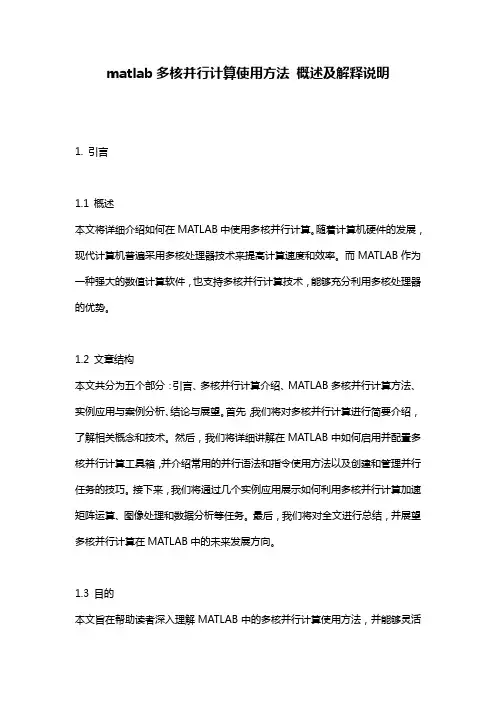
Figure 1. MEMS-based accelerometer. Image courtesy MEMSIC Inc. www.memsic.com
Figure 2. Electrostatic comb drive. Image courtesy Compliant Mechanisms Research Group, Brigham Young University. http://research.et.byu.edu/llhwww/intro/memsintro.html
MEMS devices typically consist of thin, high-aspect ratio, movable beams or electrodes suspended over a fixed electrode ( Figures 1 and 2 ). They integrate mechanical elements on silicon substrates using microfabrication.The electrode deformation caused by the ap-plication of voltage between the movable and fixed electrodes can be used for actuation, switching, and other signal and information processing functions.FEM provides a convenient tool for charac-terizing the inner workings of MEMS devices so as to predict temperatures, stresses, dy-namic response characteristics, and possible failure mechanisms.
MEMS Devices
1 Workers are MATLAB computational engines that run separately from your MATLAB session.2 MATLAB Digest www.mathworks.com
One of the most common MEMS switches is the cantilever series (Figure 3). This con-sists of beams suspended over a ground electrode.
Figure 4 shows the modeled geometry. The top electrode is 150µm in length, and 2µm in thickness. Young’s modulus E is 170 GPa, and the Poisson ratio υ is 0.34. The bottom electrode is 50µm in length, 2µm in thickness, and located 100µm from the left-most end of the top electrode. The gap be-tween the top and bottom electrodes is 2µm.
When a voltage is applied between the top electrode and the ground plane, electro-static charges are induced on the surface of the conductors, which give rise to electro-static forces acting normal to the surface of the conductors. Since the ground plane is fixed, the electrostatic forces deform only the top electrode. When the beam deforms, the charge redistributes on the surface of the conductors. The resultant electrostatic forces and the deformation of the beam also change. This process continues until a state of equilibrium is reached.
Applying FEM to Coupled Electro-Mechanical Analysis
For simplicity, we will use the relaxation-based algorithm rather than the Newton
method to couple the electrostatic and the mechanical domains2. The steps are as follows:
1. Solve the electrostatic FEA problem in the nondeformed geometry with constant po-tential V0 on the movable electrode.
2. Compute load and boundary conditions for the mechanical solution using the calcu-lated values of the charge density along the movable electrode.
The electrostatic pressure on the movable electrode is given by
aaWhere, |D|= Magnitude of the electric flux density ε = Electric permittivity next to the movable electrode 3. Solve the mechanical FEA to compute the deformation of the movable electrode. 4. Using the calculated displacement of the movable electrode, update the charge density along the movable electrode.
aaWhere,|Ddef (x)|= Magnitude of the electric flux
density in the deformed electrode |D0 (x)|= Magnitude of the electric flux
density in the undeformed electrode
G = Distance between the movable and fixed electrodes in the absence of actuation υ(x)= Displacement of the movable electrode at position x along its axis 5. Repeat steps 2 – 4 until the electrode deformation values in the last two itera-tions converge. The electrostatic analysis (step 1) involves five steps: • Draw the cantilever switch geometry. • Specify the Dirichlet boundary conditions as a constant potential of 20V to the movable electrode. • Mesh the exterior domain. • Solve for the unknown electric potential in the exterior domain. • Plot the solution (Figure 5). We can quickly perform each of these tasks via the Partial Differential Equatian Toolbox™ interface.