
多元线性回归的SPSS实现
- 格式:ppt
- 大小:922.00 KB
- 文档页数:46

t i e an dl l t 多元回归分析在大多数的实际问题中,影响因变量的因素不是一个而是多个,我们称这类回问题为多元回归分析。
可以建立因变量y 与各自变量x j (j=1,2,3,…,n)之间的多元线性回归模型:其中:b 0是回归常数;b k (k =1,2,3,…,n)是回归参数;e 是随机误差。
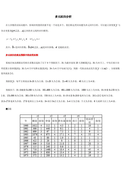
多元回归在病虫预报中的应用实例:某地区病虫测报站用相关系数法选取了以下4个预报因子;x 1为最多连续10天诱蛾量(头);x 2为4月上、中旬百束小谷草把累计落卵量(块);x 3为4月中旬降水量(毫米),x 4为4月中旬雨日(天);预报一代粘虫幼虫发生量y (头/m2)。
分级别数值列成表2-1。
预报量y :每平方米幼虫0~10头为1级,11~20头为2级,21~40头为3级,40头以上为4级。
预报因子:x 1诱蛾量0~300头为l 级,301~600头为2级,601~1000头为3级,1000头以上为4级;x 2卵量0~150块为1级,15l~300块为2级,301~550块为3级,550块以上为4级;x 3降水量0~10.0毫米为1级,10.1~13.2毫米为2级,13.3~17.0毫米为3级,17.0毫米以上为4级;x 4雨日0~2天为1级,3~4天为2级,5天为3级,6天或6天以上为4级。
表2-1x 1x 2x 3x 4y 年 蛾量 级别 卵量 级别 降水量 级别 雨日 级别 幼虫密度级别1960102241121 4.31211011961300144030.111141196269936717.511191196318764675417.14745541965431801 1.9121111966422220101013119678063510311.82322831976115124020.612171197171831460418.444245419728033630413.433226319735722280213.224216219742641330342.243219219751981165271.84532331976461214017.515328319777693640444.7432444197825516510101112数据保存在“DATA6-5.SAV”文件中。
线性回归分析的SPSS操作本节内容主要介绍如何确定并建立线性回归方程。
包括只有一个自变量的一元线性回归和和含有多个自变量的多元线性回归。
为了确保所建立的回归方程符合线性标准,在进行回归分析之前,我们往往需要对因变量与自变量进行线性检验。
也就是类似于相关分析一章中讲过的借助于散点图对变量间的关系进行粗略的线性检验,这里不再重复。
另外,通过散点图还可以发现数据中的奇异值,对散点图中表示的可能的奇异值需要认真检查这一数据的合理性。
1、一元线性回归分析1.数据以本章第三节例3的数据为例,简单介绍利用SPSS如何进行一元线性回归分析。
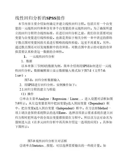
数据编辑窗口显示数据输入格式如下图7-8(文件7-6-1.sav):图7-8:回归分析数据输入2.用SPSS进行回归分析,实例操作如下:2.1.回归方程的建立与检验(1)操作①单击主菜单Analyze / Regression / Linear…,进入设置对话框如图7-9所示。
从左边变量表列中把因变量y选入到因变量(Dependent)框中,把自变量x选入到自变量(Independent)框中。
在方法即Method一项上请注意保持系统默认的选项Enter,选择该项表示要求系统在建立回归方程时把所选中的全部自变量都保留在方程中。
所以该方法可命名为强制进入法(在多元回归分析中再具体介绍这一选项的应用)。
具体如下图所示:图7-9 线性回归分析主对话框②请单击Statistics…按钮,可以选择需要输出的一些统计量。
如Regression Coefficients(回归系数)中的Estimates,可以输出回归系数及相关统计量,包括回归系数B、标准误、标准化回归系数BETA、T值及显著性水平等。
Model fit项可输出相关系数R,测定系数R2,调整系数、估计标准误及方差分析表。
上述两项为默认选项,请注意保持选中。
设置如图7-10所示。
设置完成后点击Continue返回主对话框。
图7-10:线性回归分析的Statistics选项图7-11:线性回归分析的Options选项回归方程建立后,除了需要对方程的显著性进行检验外,还需要检验所建立的方程是否违反回归分析的假定,为此需进行多项残差分析。

SPSS数据统计分析与实践主讲:周涛副教授北京师范大学资源学院2007-11-20教学网站:/Courses/SPSS1第十三章多元线性回归本章内容:一、多元线性模型基本原理二、SPSS实例2Chapter Topicsz The Multiple Regression Modelz Contribution of Individual Independent Variablesz Coefficient of Determinationz Model Building34The Multiple Regression Modelipi p i i i X X X Y εββββ++•••+++=22110Relationship between 1 dependent & 2 or more independent variables is a linear functionPopulation Y-interceptPopulation slopesDependent (Response) variable for sampleIndependent (Explanatory) variables for sample modelRandom Erroripi p i i i e X b X b X b b Y ˆ++•••+++=221105Sample Multiple Regression ModelX 2X 1Ypi p i i i X b X b X b b Yˆ+•••+++=22110ipi p i i i e X b X b X b b Y ++•••+++=22110e i6Oil (Gal)Temp Insulation 275.30403363.80273164.30401040.8073694.30646230.90346366.7096300.60810237.802310121.4063331.406510203.50416441.10213323.0038352.505810Multiple Regression Model: Example(0F)Develop a model forestimating heating oil used for a single family home in the month of January based on averagetemperature and amount of insulation in inches.7三维散点图与散点图矩阵regression_oil.sav8Sample Regression Model: Examplepip i i i X b X b X b b Y ˆ+•••+++=22110Co efficien ts In te rce p t562.1510092X V a ria b le 1-5.436580588X V a ria b le 2-20.01232067Outputi i i X .X ..Yˆ21012204375151562−−=For each degree increase in temperature, the average amount of heating oil used is decreased by 5.437 gallons, holding insulationconstant.For each increase in one inch of insulation, the use of heating oil is decreased by 20.012 gallons, holding temperatureconstant.9Using The Model to Make Predictions96927860122030437515156201220437515156221....X .X ..Y ˆii i =•−•−=−−=Estimate the average amount of heating oil used for a home if the average temperature is 300 and the insulation is 6 inches.The estimated heating oilused is 278.97 gallons10Coefficient of Multiple DeterminationRegression S tatisticsM ultiple R 0.982654757R S quare 0.965610371A djus ted R S quare 0.959878766S tandard E rror 26.01378323O bs ervations 15OutputSSTSSR r ,Y =212Adjusted r 2•reflects the number of explanatoryvariables and sample size•is smaller than r 2RMSE MS n n p R adjtotal 2211111=−=−−−−−()11DeterminationRegression S tatisticsM ultiple R 0.982654757R S quare 0.965610371A djus ted R S quare 0.959878766S tandard E rror 26.01378323O bs ervations 15Output复相关系数(多元相关系数)•表示模型中所有自变量(x1,x2)与应变量y 之间线性回归关系的密切程度•实际上它是yi 与其估计值(y hat )的简单线性相关系数DeterminationRegression S tatisticsM ultiple R0.982654757R S quare0.965610371A djus ted R S quare0.959878766S tandard E rror26.01378323O bs ervations1512Residual Plots∧z Residuals Vs Y iz May need to transform Y variablez Residuals Vs X1z May need to transform X1variablez Residuals Vs X2z May need to transform X2variablez Residuals Vs Timez May have autocorrelation1314Insulation Residual Plot024681012Residual Plots: ExampleOutputNo Discernable PatternTemperature Residual Plot-60-40-200204060020406080R e s i d u a l sTesting for OverallSignificance•Shows if there is a linear relationship between all of the X variables together and Y•Use F test Statistic•Hypotheses:H0: β1= β2 = …= βp= 0 (No linear relationship) H1: At least one βi≠0 ( At least one independentvariable affects Y)15Output: ExampleANOVAdf SS M S F Significance F Re gre ssion2228014.6114007.3168.4712028 1.65411E-09 Re sidua l128120.603676.7169Tota l14236135.2p = 2, the number ofexplanatory variables n -1MRSMSEp value= F Test Statistic1617F0 3.89z H 0: β1= β2 = …= βp = 0z H 1: At least one βI ≠0z α= .05z df = 2 and 12z Critical Value(s):Test Statistic:Decision:Conclusion:Reject at α= 0.05There is evidence that At least one independentvariable affects Yα= 0.05F =Example Solution168.47( Output)Test for Significance:Individual Variables•Shows if there is a linear relationship between thevariable X i and Y•Use t test Statistic•Hypotheses:H0: βi = 0 (No linear relationship)H1: βi≠0 (Linear relationship between X i and Y)18t Test StatisticOutput: Examplet Test Statistic for X1(Temperature) Co efficien ts S tan d ard E rro r t S tatIn te rce p t562.15100921.0931043326.65094X V a ria b le 1-5.43658060.336216167-16.1699X V a ria b le 2-20.012321 2.342505227-8.54313 t Test Statistic for X2(Insulation)1920z H 0: β1= 0H 1: β1≠0z df = 12Critical Value(s):Test Statistic:Decision:Conclusion:Reject H 0at α= 0.05There is evidence of a significant effect of temperature on oil consumption.0 2.1788-2.1788.025Reject H 0Reject H 0.025Does temperature have a significant effect on monthlyconsumption of heating oil? Test at α= 0.05.t Test : Example Solutiont Test Statistic = -16.169921Confidence Interval Estimate For The SlopeProvide the 95% confidence interval for the population slope β1 (the effect of temperature on oil consumption).111b p n S t b −−±CoefficientsLower 95%Upper 95%Intercept 562.151009516.1930837608.108935X Variable 1-5.4365806-6.169132673-4.7040285X Variable 2-20.012321-25.11620102-14.90844-6.169≤β1≤-4.704The average consumption of oil is reduced by between4.7 gallons to 6.17 gallons per each increase of 10 F.22zContribution of One X i to Model (holding all others constant)zDenote by SSR(X i | all variables except i )SSR : extra sum of squares , which measures the marginal reduction in the error sum of squares when one or several predictor variables are added to the regression model, given that other predictor variables are already in the modelz= Coefficient of partial determination of X 1 with Y holding X 2constantz Evaluate Separate ModelszUseful in Selecting Independent VariablesTesting Portions of Model221.Y r23Testing Portions of Model: SSRContribution of X 1given X 2has been included:SSR(X 1⎮X 2)=SSR(X 1and X 2)-SSR(X 2)From ANOVA section of regression fori i i X b X b b Yˆ22110++=From ANOVA section ofregression fori i X b b Yˆ220+=Partial F Test For Contribution of Xiz Hypotheses:z H0:Variable X i does not significantly improvethe model given all others includedH1: Variable Xisignificantly improves the model given all others includedz Test Statistic:z F=MSE )othersallX(SSRiWith df= 1 and (n -p -1)2425Coefficient of Partial Determination)X X (SSR )X and X (SSR SST )X X (SSR r .Y 212121221+−=i i i X b X b b Yˆ22110++=From ANOVA section of regression forFrom ANOVA section ofregression fori i X b b Yˆ220+=ExampleTest at the α= .05 levelto determine if thevariable of averagetemperaturesignificantly improvesthe model given thatinsulation is included.2627ExampleH 0: X 1 does not improve model (X 2included)H 1: X 1does improve modelα= .05, df = 1 and 12Critical Value = 4.75A N O V A S SR e g r e ssi o n51076.47R e si d u a l 185058.8T o ta l236135.27176760765101522821,,,MSE )X X (SSR F −==ANOVA SS M SRegression 228014.6263114007.313Residual 8120.603016676.716918Total236135.2293(For X 1and X 2)(For X 2)= 261.47Conclusion: Reject H 0. X 1 does improve model28Collinearityz High Correlation Between Explanatory Variablesz No New Information Provided z Leads to Unstable CoefficientszDepending on the explanatory variableszVIF Used to Measure CollinearityVIF :Variance Inflation Factor (方差膨胀因子),R VIF jj 211−=2j R = Coefficient of MultipleDetermination of X j with all the othersModel Buildingz Goal is to Develop Model with Fewest Explanatory Variablesz Easier to interpretz Lower probability of collinearityz Stepwise Regression Procedurez Provide limited evaluation of alternativemodelsz Best-Subset Approachz Uses the C p Statistic2930Model Building (C p Statistic )zC p Statistic 由C.L. Mallows 于1964年提出np MSE SSE MSE p n MSE MSE p C mp mm p p −+=−−+=2))((式中MSE p 指模型中含有p 个参数(包括常熟项)时的误差均方,MSE m 为所有自变量均引入模型时的误差均方。

SPSS多元线性回归分析实例操作步骤多元线性回归是一种常用的统计分析方法,用于探究多个自变量对因变量的影响程度。
SPSS(Statistical Package for the Social Sciences)是一款常用的统计软件,可以进行多元线性回归分析,并提供了简便易用的操作界面。
本文将介绍SPSS中进行多元线性回归分析的实例操作步骤,帮助您快速掌握该分析方法的使用。
步骤一:准备数据在进行多元线性回归分析之前,首先需要准备好相关的数据。
数据应包含一个或多个自变量和一个因变量,以便进行回归分析。
数据可以来自实验、调查或其他来源,但应确保数据的质量和可靠性。
步骤二:导入数据在SPSS软件中,打开或创建一个新的数据集,然后将准备好的数据导入到数据集中。
可以通过导入Excel、CSV等格式的文件或手动输入数据的方式进行数据导入。
确保数据被正确地导入到SPSS中,并正确地显示在数据集的各个变量列中。
步骤三:进行多元线性回归分析在SPSS软件中,通过依次点击"分析"-"回归"-"线性",打开线性回归分析对话框。
在对话框中,将因变量和自变量移入相应的输入框中。
可以使用鼠标拖拽或双击变量名称来快速进行变量的移动。
步骤四:设置分析选项在线性回归分析对话框中,可以设置一些分析选项,以满足具体的分析需求。
例如,可以选择是否计算标准化回归权重、残差和预测值,并选择是否进行方差分析和共线性统计检验等。
根据需要,适当调整这些选项。
步骤五:获取多元线性回归分析结果点击对话框中的"确定"按钮后,SPSS将自动进行多元线性回归分析,并生成相应的分析结果。
结果包括回归系数、显著性检验、残差统计和模型拟合度等信息,这些信息可以帮助我们理解自变量对因变量的贡献情况和模型的拟合程度。
步骤六:解读多元线性回归分析结果在获取多元线性回归分析结果之后,需要对结果进行解读,以得出准确的结论。