ncl操作手册

ncl绘图基本流程下载温馨提示:该文档是我店铺精心编制而成，希望大家下载以后，能够帮助大家解决实际的问题。

文档下载后可定制随意修改，请根据实际需要进行相应的调整和使用，谢谢!并且，本店铺为大家提供各种各样类型的实用资料，如教育随笔、日记赏析、句子摘抄、古诗大全、经典美文、话题作文、工作总结、词语解析、文案摘录、其他资料等等，如想了解不同资料格式和写法，敬请关注!Download tips: This document is carefully compiled by theeditor. I hope that after you download them,they can help yousolve practical problems. The document can be customized andmodified after downloading,please adjust and use it according toactual needs, thank you!In addition, our shop provides you with various types ofpractical materials,such as educational essays, diaryappreciation,sentence excerpts,ancient poems,classic articles,topic composition,work summary,word parsing,copy excerpts,other materials and so on,want to know different data formats andwriting methods,please pay attention!NCL（NCAR Command Language）是一种专门用于气象、海洋和气候数据处理和可视化的编程语言。

图文详解Windows平台上NCL的安装NCL在Linux下的安装非常容易，只需下载适当版本的文件，设置好环境变量即可使用。

NCL在Windows下的安装则要麻烦一些，需要先安装一个虚拟Linux环境（Cygwin/X）。

以下内容详细介绍NCL在Windows平台上的安装过程，希望仅具备Windows基本操作技能的用户也能轻松安装NCL。

一、NCL简介二、准备工作三、安装Cygwin/X四、熟悉Cygwin/X环境五、安装NCL六、运行NCL范例七、语法高亮显示（此部分供有兴趣的用户参考）八、.hluresfile文件（此部分供有兴趣的用户参考）九、FAQ十、获取帮助一、NCL简介NCL（NCAR Command Language）是由NCAR的“Computational & Information Systems Laboratory”开发的。

NCL是一种编程语言，专门用于分析和可视化数据。

主要用于以下三个领域：文件输入/输出（File input and output）：资料处理（Data processing）：图形显示（Graphical display）：可生出出版级别的黑白、灰度或彩色图。

从5.0起，NCL和NCAR Graphics已经打包在一起发行。

2009年3月4日，NCL发布了最新的5.1.0版，该版本更新了地图投影，修正了一些bug，增加了更多的函数及资源。

下图为新增的含中国省界的地图（见图1-1）。

二、准备工作2.1 安装环境安装环境为WinXP Professional SP3，并做如下假定：计算机名：TEAM用户名：Grissom安装目录：D:\download用户在实际安装中，请根据自己系统的信息替换本教程中的计算机名和用户名。

特别说明：用户名中不能出现空格，否则会在使用中出现一些问题。

2.2 下载Cygwin/XCygwin/X=Cygwin+X。

通俗地说，Cygwin/X可以在Windows平台上实现命令行+图形的Linux模拟环境。

服务器操作手册（LMCB Service tool manual）受控文件编号：Field Component Ma nual更改页版本：第A版页码：第1/1 页TrustCon-CL日期：2006-04-25更改记录序号更改文件号更改内容描述更改日期签名1 首次归档说明：版本：第A版页码：第 1 /18 页TrustCon-CL日期：2006-04-25目录1 简介2 结构说明3 LMCB SVT1 菜单系统4 LMCB SVT2 菜单系统5 快捷键6 服务器功能版本：第A版页码：第2页TrustCon-CL日期：2006-02-251. 简介在TrustCon-CL控制柜中，服务器可以用来查看和设置所有与电梯和驱动相关状态和参数；—监控软件状态，系统输入和输出，系统信息—设置参数等所有的参数设置及状态参看，都在3子菜单下面：1—SYSTEM(SVT1) 电梯的逻辑控制菜单2—TOOL(SVT1) 一些其它的工具菜单3—DRIVE(SVT2) 变频驱动菜单2. 结构说明服务器进入SVT1后界面如下图所示：版本：第A版页码：第3页TrustCon-CL日期：2006-02-25 下图是进入SVT2的界面，按钮功能与进入SVT1时相同；版本：第A版页码：第4页TrustCon-CL日期：2006-02-25 3 LMCB SVT1 菜单系统用服务器按相应的数字（0－9）键可以进入对应的菜单；如果需要往前翻页可以按“GOON”,如果往后翻页可以按“GOBACK”如果需要进入某一功能或对参数进行确认按“ENTER”版本：第A版页码：第5页TrustCon-CL日期：2006-02-25 3.1 SVT1 系统菜单版本：第A版页码：第6页TrustCon-CL日期：2006-02-25 3.2 SVT1 工具菜单3.3 服务器上电菜单如果按“M”键则显示下面界面：版本：第A版页码：第7页TrustCon-CL日期：2006-02-253.3 SVT1菜单3.3.1按“M”键进入如下界面(M)在此界面如果按照下表按键，则会出现相应的界面：按键顺序相应界面1 进入System菜单2 进入Tools菜单SHIFT+2(UP)GOON或SHIFT+GOONSHIFT+1(ON)SHIFT+13.3.2按“1”键进入系统菜单（M-1如下界面）版本：第A版页码：第8页TrustCon-CL日期：2006-02-25 在此界面如果按照下表按键，则会出现相应的界面：按键顺序相应界面1 进入Status菜单2 进入Test菜单3 进入Setup菜单M 退回到最上一级菜单Clear 退回上一级菜单3.3.3按“1”键进入状态菜单（M-1-1如下界面）在此界面如果按照下表按键，则会出现相应的界面：按键顺序相应界面1 进入Calls菜单2 进入Input菜单3 进入Output菜单4 进入Group菜单5 进入ICSS菜单6 进入Cmd菜单GOON或可以往前或往后翻页SHIFT+GOONM 返回到最上一级菜单F 返回到第二级菜单Clear 退回上一级菜单版本：第A版页码：第9页TrustCon-CL日期：2006-02-25 3.3.4按“2”键进入测试菜单（M-1-2如下界面）在此界面如果按照下表按键，则会出现相应的界面：按键顺序相应界面1 进入Events菜单2 进入Diagnosis菜单3 进入Part菜单4 进入RSL菜单5 进入Selftest菜单可以往前或往后翻页GOON或SHIFT+GOONM 返回到最上一级菜单F 返回到第二级菜单Clear 退回上一级菜单3.3.5按“3”键进入设置菜单（M-1-3如下界面）版本：第A版页码：第10页TrustCon-CL日期：2006-02-25在此界面如果按照下表按键，则会出现相应的界面：按键顺序相应界面1 进入INSTALL菜单2 进入RSL菜单3 进入ALLOWED菜单4 进入POS.菜单5 进入DCS-RUN菜单6 进入ELD-FUNC.菜单可以往前或往后翻页GOON或SHIFT+GOONM 返回到最上一级菜单F 返回到第二级菜单Clear 退回上一级菜单版本：第A版页码：第11页TrustCon-CL日期：2006-02-25 3.3.6按“1”键进入设置菜单（M-1-3-1如下界面）在此界面如果按照下表按键，则会出现相应的界面：按键顺序相应界面1－9 进入System至Security菜单可以往前或往后翻页GOON或SHIFT+GOONM 返回到最上一级菜单F 返回到第二级菜单S 返回到设置菜单Clear 退回上一级菜单3.3.7按“3”键进入设置菜单（M-1-3-3如下界面）在此界面如果按照下表按键，则会出现相应的界面：版本：第A版页码：第12页TrustCon-CL日期：2006-02-25 按键顺序相应界面1 进入Allowed-Enable菜单3 进入ALLOWED-Menu菜单ENTER 确认所显示的功能可以往前或往后翻页GOON或着SHIFT+GOONM 返回到最上一级菜单F 返回到第二级菜单S 返回到设置菜单Clear 退回上一级菜单3.4按“2”键进入设置菜单（M-2如下界面）按键顺序相应界面1 进入Search IO菜单2,3或者9 访问功能Erase IO, Setup INST或者Opr.MemoryENTER 确认所显示的功能GOON或可以往前或往后翻页SHIFT+GOONF 返回到第二级菜单S 返回到设置菜单Clear 退回上一级菜单4 LMCB SVT2功能版本：第 A 版 页码：第 13 页 日期：2006-02-25TrustCon-CL功能树表如下MODULEDBSS = 331 = MONITOR33 = SETUP 311 = CATEGORY A 312 = CATEGORY B 313 = CATEGORY C 32 = DIAGNOSTICS 321 = CURRENT FAULT LOG322 = SAVED FAULT LOG323 = CLEAR CURRENT FAULT LOG331 = CONTRACT DATA 3311 = FIELD ADJUST3312 = VELOCITY REGULATOR 3313 = BRAKE / DBR 3314= MOTOR 3315= I REGULATOR 3316 = TIMIMG3317 = DRIVE SCALING 3318 = CLOCKS & PWM 333 = SYSTEM PARA.INI 332 = MOTOR TUNE 314 = POSITION324 =CLEAR SAVED FAULT3319 = ENHANCED 335 = LOAD3310 = level334 = Height Learn按键顺序相应界面版本：第A版页码：第14页TrustCon-CL日期：2006-02-251 进入监控菜单2 进入事件记录菜单3 进入参数设置菜单M 退回上一级菜单4.1监控菜单按键顺序相应界面1 进入监控类别1菜单2 进入监控类别2菜单3 进入监控类别3菜单M 返回最上一级菜单4.2事件记录菜单按键顺序相应界面1 进入当前故障菜单2 进入保存的故障菜单3 复位当前故障4 复位所有保存的故障M 返回最上一级菜单4.3参数设置菜单按键顺序相应界面1 进入常用参数菜单2 进入电机位置自学习菜单3 进入参数初始化菜单4 进入井道自学习菜单5 进入称重装置设置菜单M 返回最上一级菜单4.4常用参数菜单版本：第A版页码：第15页TrustCon-CL日期：2006-02-25按键顺序相应界面1 进入工地调整参数菜单2 进入速度调整参数菜单3 进入制动器开关菜单4 进入电机参数菜单5 进入电流调整参数菜单6 进入时间参数菜单7 进入驱动器容量参数菜单8 进入定时及PWM相关参数菜单9 进入电梯机械参数设置菜单0 进入平层参数菜单M 返回最上一级菜单5 快捷键S4-S9快捷键能快速的进入服务器中的一些常用的特定功能。

2011.3.231.知道了ncl软件的脚本后缀为.ncl，运行该.ncl脚本的命令为：ncl xxx.ncl2.当然在这之前需先进入要使用的数据所在的目录下：cd /wk3/zhang/MITAG ;然后再进入远程机上的ncl软件，即输入ncl就进入了该软件！（与grads类似）3.将.grb2文件转化为.nc格式的文件：先建立一个脚本表示打开某文件的函数：addfile（"文件绝对或相对路径名xxx.grib2","r"）其中第二个可以写成"r"（只是可读）、"w"（可读可写）、"c"（若前面打开的文件不存在，则创建了一个新文件，且该文件默认可写入新的东东哦!!）"r" for read-only,"w"for read-write,"c" is set,assuming the user has permissions to write in the specified directory and the format is writable, the file is created if it does not exit.If it does exit,an error message is printed and the default missing value for files is returned.Opens a data file that is(or is to be)written in a supported file format.其中"r":表示该打开的文件可读4.在NCL的脚本文件.ncl中；于GrADS中的*起到一样的作用为注释行的意思，其后的语句是不被执行的5.NCL中执行外部命令的函数：system("外部命令的完整形式")Executes a shell command.6.NCL中也可以写循环：do i=0, dimsizes(names)-1ncdf_out->$names(i)$=grib_in->$name(i)$end do把grb2的大文件转化成.nc的确不是一个好主意因为转化成.nc之后太大了，而且转化过程也太过漫长了啊！！！[NCL]2.NCL简单语法、读取nc文件[这个贴子最后由first在2007/04/14 12:42pm 编辑]进入ncl的两种方法：1.直接在shell命令行输入ncl，就能进入ncl，然后一条一条执行命令，这种是交互式的执行方式。

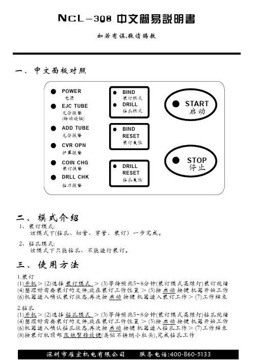
NCL-308中文简易说明书一、中文面板对照二、模式介绍1、装订模式:该模式下(钻孔、切管、穿管、装订）一步完成。

2、钻孔模式:
该模式下只能钻孔、不能进行装订。

三、使用方法
11.装订
()开机＞()选择＞()等待预热~分钟(装订模式亮绿灯)装订就绪
()整理好需要装订的文件,放在装订工作位置＞()按按键机器开始工作
()机器进入确认装订状态,再次按按键机器进入装订工作＞()工作结束
23584567装订模式启动启动218.钻孔()按装订机顶部(类似不锈纲小杠头),完成钻孔工作
开机
压纸臂释放键＞()选择＞()等待预热~分钟(装订模式亮绿灯)钻孔就绪
()整理好需要装订的文件,放在装订工作位置＞()按按键机器开始工作
()机器进入确认钻孔状态,再次按按键机器进入钻孔工作＞()工作结束
()23584567钻孔模式启动启动如若有误,敬请赐教。

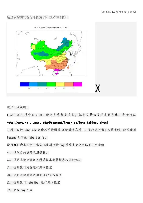
这里以绘制气温分布图为例，效果如下图：X这里几点说明：1.ncl不支持中文显示，所有文字都是英文，但是支持很多样式的字体，参考网址http://www.ncl。

ucar。

edu/Document/Graphics/font_tables。

shtml2.图下方的labelbar只能在图的周围,不能放置在图内。

要想显示图下方的图例，就要使用legend而不是labelbar了。

使用NCL脚本绘制一张如上图所示的png图片主要分为以下几个步骤一、读取各站点的气温数据。

二、将站点数据使用各种差值函数转换成格点数据。

三、使用源对地图进行基本设置四、使用源对等值线填充进行基本设置五、使用源对labelbar进行基本设置六、生成png图片接下来将按照这几个步骤,详细介绍。

一、读取各站点的气温数据NCL支持的数据格式主要有netCDF文件(.nc .cdf）、HDF4(。

hd 。

hdf）、HDF4-EOS（.hdfeos)、GRID-1/GRIB-2(。

grb.grib）、CCMHistory Tape(。

ecm)，除此之外呢，它支持二进制文件和ascii文件，这两者是我们最熟悉的。

这里我们使用ascii文件，更多文件读取方式参考http：//www。

ncl.ucar。

edu/Applications/list_io.shtml为了批量生成产品图片，需要配置文件设置数据来源以及图片生成后存放位置.config.txt 文件如下：One Hour of Temperature2010111502./t1//root/WorkSpace/MICAPS_surface/t1/10111502.000第一行是标题第二行是输出png图路径第三行是输入数据文件路径第四行是数据文件名在NCL脚本（temperature.ncl）中使用以下几行代码就可以了filepath = '。

/config。

txt' ;参数文件路径argu = asciiread（filepath，-1，’string’）；以字符串形式读取参数文件入数组argu lines = asciiread（argu（2)+argu（3）,-1，'string’) ；以字符串形式读取数据文件入数组linesstation = stringtofloat(str_get_field（lines（3:：），1,' '））；从数组lines中获取站号lon = stringtofloat(str_get_field(lines（3：:)，2,’ ’)） ;从数组lines中获取经度值lonlat = stringtofloat(str_get_field(lines(3：:）,3,’ '）） ;从数组lines中获取纬度值latheight = stringtofloat（str_get_field（lines（3：：），4，' ')）；从数组lines 中获取海拔高度R = stringtofloat（str_get_field(lines(3：:）,5,' ’）) ；从数组lines中获取站点数据值由于数据文件10111502。

NCARG_ROOT美元/ bin添加到你的搜索路径。

为了运行NCL脚本显示他们的直接输出一个X11窗口,你需要显示环境变量设置正确。

通常你可以测试这个马上通过调用一个X应用程序是否这告诉xander的机器,可以让程序由“巴菲”被显示在监视器。

再一次,与上面的NCARG_ROOT环境变量中,您可能想要将这些行添加到适当的”。

在您的主目录*”文件。

如果上面的不工作,那么请检查与您的系统管理员。

”。

在您的主目录hluresfile”文件。

为了更好地定制NCL图形环境,我们强烈建议你复制一个.hluresfile到您的主目录。

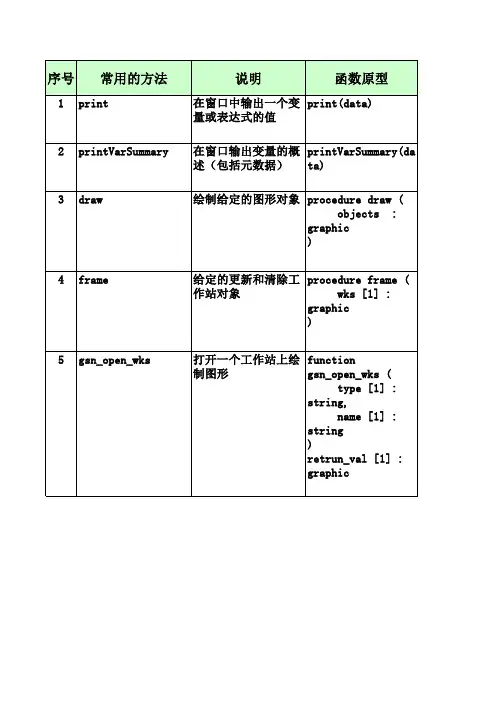
您可以定制这个文件对你的喜欢,但至少,你想改变默认的Explanation of example 1Load the NCL script that contains the functions and procedures (the ones that start with "gsn_") that are used in this example. The statement in NCL works much like include works in C and Fortran 90 programs.Start every NCL script with the statement and end it with the statement.variable, and the second argument its type. In this case, the two new statements are redundant, because in NCL you can declare variables by initializing them (as you do in the next two lines).For an overview of NCL's variable types, see the "NCL data types overview" section of the NCL Reference Manual.and terminated by "/)". Arrays in NCL are modeled after arrays in the C programming language; that is, they are row-major and begin at index 0 (instead of column-major and index 1 as in Fortran).an NCAR Graphics metafile (NCGM), or a PostScript file (regular, encapsulated, or encapsulated interchange).The function gsn_open_wks opens one of these types of workstations so you can draw graphics to it. The first argument (a string) indicates where you want the graphical output drawn ("x11" for an X11 window, "ncgm" for an NCGM, and "ps", "eps", or "epsi" for a PostScript file). The second argument (also a string) determines the name of the file if you draw the graphical output to an NCGM or a PostScript file (name.ncgm for an NCGM file, and name.{ps,eps,epsi} for a PostScript file, where name is the second string you pass in). The second argument also comes into playwhen resource files are discussed in example 8 and 9.The value returned from gsn_open_wks is a special variable of type graphic, which is an NCL variable type to define graphical objects.to do anything with this return value). The first argument is the workstation you want to draw the XY plot to (the variable returned from the previous call to gsn_open_wks). The next two arguments are the variables containing the X and Y arrays that you want to plot. These two arguments can be of type float, double, or integer and can be 1-dimensional or multi-dimensional (explained below). The last argument is a logical value indicating whether you have set any "resources" for changing the look of a plot. To get the default XY plot that NCL provides, pass the value False for the last argument (in NCL,logical values are set with the special keywords True or False, which both must be capitalized).The gsn_xy function draws the XY plot with tick marks selected at "nice" values. No title or X/Y axis labels are provided in the default plot, but these can be easily added as shown in the next few plots. You can also change the style of the tick marks as shown in example 7.By default, when a plot is drawn to an X11 window or an NCGM file, it has a black background and a white foreground. If a plot is drawn to a PostScript file, it has a white background and a black foreground. In later examples, you will learn how to specify the background and foreground colors, and when you do this, the plot has the same colors, no matter which workstation you draw it to.Since you opened a workstation type of "x11", the gsn_xy function produces an X11 window on which you need to click with the left mouse button to advance to the next frame.Line 14:Draw an XY plot with three curves, each curve having nine points.time you are not using new to declare the array, because in NCL you can create variables by assigning values to them. NCL is able to determine the dimensionality and type of a variable by the way it is initialized.they may also contain ancillary information about the variable. This additional information is often called "metadata." Metadata is divided into three categories: attributes, named dimensions, and coordinate variables.Variables can have an unlimited number of attributes assigned to them, and each attribute is assigned to a variable using the "@" symbol.In lines 20-21, you are creating an attribute called "long_name" for both the x and y2 variables. For more information on variable properties in NCL, see the "Variables" section in the "Basics."By default, if an attribute called "long_name" is set for either the X or Y data arrays, (as is commonly done in netCDF files), then gsn_xy uses this attribute to label the X and/or Y axis in the XY plot (unless you have overridden this by setting resources as shown below).the values in the x array with the values in each of the three curves in the y2 array. If a 3 x 9 X array had been declared in addition to the 3 x 9 Y array, then each value in the Y array would have been paired with the corresponding value in the X array.Note that if more than one curve is drawn in an XY plot, then gsn_xy draws each curve with a unique dash pattern. There are 16 different dash patterns available; see the list of "dash patterns" in the graphics documentation.Note the new X and Y axis labels that result from the attribute "long_name" being set for each axis.line colors and thicknesses, adding titles, changing fonts, creating label bars and legends, changing map projections, modifying the size of a plot, masking out certain areas, etc. There are also resources for changing the data of a plot, like setting minimum and maximum values, selecting strides or subsets of data, and setting missing values.Most resources have default values that are either hard-coded or set dynamically by NCL when you run the NCL script. For example, the line thickness for a curve is hard-coded to a value of 1.0, but the minimum and maximum values of a curve are set dynamically according to the actual minimum and maximum data values used in the XY plot. You only need to set a resource if you want to change its default value.Resources are grouped by the type of graphical object or data they describe, and these groupings are discussed here and in other examples.To set resources for use by the gsn_* suite of functions, first define a variable of type logical and set its value to True, then specify the resources as attributes of this logical variable. As stated above, a variable can have an unlimited number of attributes. This variable that you create should then get passed to the appropriate gsn_* plotting routine for the resources to take effect.Important note: This method for setting resources is specific to the gsn_* suite of functions and procedures. Setting resources using straight NCL code is quite different, and is covered in the "Going beyond the basics" section of this document.colors specified here are represented by integer index values, where each index maps to a color in a predefined color table (also called a "color map"). Since a color table has not been defined in this example, a default color table with 32 indices is provided by NCL (later examples will show how to create your own color map). To see the default color table, go to the "Color tables" section of the NCAR Graphics Reference Manual. In the default color table, the integer values 2, 3, and 4 represent the colors "red", "green", and "blue" respectively.If you had wanted the same line color for each curve, but wanted it something other than "1", then you could have used the singular resource, xyLineColor.XY plot resources belong to the "XyPlot" group and start with the letters "xy". Each XyPlot resource is documented with its type and its default value in the XyPlot resource descriptions.thickness and a value of 5.0 increases the line thickness by a factor of 5, and so on. Again, you could have used the singularresource xyLineThicknessF to set all the curves to the same thickness.and/or lines to draw each curve.Since you are creating the same plot as before, you want to keep the same resources that you set for the previous XY plot. You can just add more attributes to the resources variable to customize the plot some more.If you had wanted to go back to all the default resources before creating the next XY plot, you could have either used a new variable name for the resources, or deleted the current list of resources with the delete(resources) command and started over with a new list.and start with "ti.an index into a font table. A table of all the available fonts along with their names and index values appears in the "Font table" section of the NCAR Graphics Reference Manual.Note that predefined strings, like those listed in the font table, are case-insensitive, and that you could have specified the font with "helvetica" or "HELVETICA" or any another combination of uppercase and lowercase characters.lines that can be drawn: regular lines ("Lines"), markers only ("Markers"), and lines with markers ("MarkLines"). In this plot, you are using this resource to invoke all three kinds of lines. The xyMarkers resource defines the type of markers you want to use. There are seventeen marker styles to choose from.get the same marker color and size for all the lines that have markers. The default marker size is 0.01, so a value of 0.03 triples the marker size.you can use environment variables in NCL in a file path name by prefixing a "$" to the name.The first argument of asciiread is the file name, the second argument (a 1-dimensional integer array) is the dimensionality of the data you are reading in, and the third argument (a string) is the type of the data. In this case, the ASCII data file has 4 columns of data with 129 rows each, so a dimensionality of (/129,4/) is used to read in the data.values from data (remember, arrays in NCL start at index 0, not index 1). If you had wanted to select elements 50 to 100 of the first set of 129 values, you would have used the notation "(49:99,0)".to represent longitude values from 0.0 to 360.0 in steps of 360/128, you need to convert each value by subtracting 1 and multiplying it by 360/128. In NCL, you can do scalar arithmetic on a whole array using the same notation as if it were a scalar value. You can also multiply, divide, add, and subtract arrays in one step as long as they are the appropriate size for doing such array computations.Lines 63-64 could also have been combined into one line:the delete command. If you plan to set some new resources, the variable resources must be again set to True, since delete removes all information relating to it. You could have also just used a new variable name.to customize how to label the XY plot curves (there are no labels by default). You can indicate what labels you want withthe xyExplicitLabels resource. The xyLineLabel* resources used here change the font size and color of the line labels.of the NCL script, but it's a good idea to get in the habit of cleaning up variables that you no longer need.Example 7 - two XY plots on one frameThis example illustrates the use of the routines ftcurvp and ftcurvpi and creates two XY plots on the same frame. It also illustrates how to draw text and polylines in a specified area of the viewport.The function ftcurvp calculates an interpolatory spline under tension through a sequence of functional values for a periodic function, and ftcurvpi calculates an integral of an interpolatory spline between two specified points.To run this example, you must download the following file:gsun07n.ncland then type:ncl gsun07n.ncl(Click on frame to see it enlarged.)value to start at, the floating point value to end with, and the number of evenly spaced points to create in between.xi is a 1-dimensional array (10 elements) containing the abscissae for the input function, yi. The variable period is a scalar value specifying the period of the input function, and xo is a 1-dimensional array containing the abscissae for the interpolated values. ftcurvp returns a 1-dimensional array thatcontaining the lower limit of the integration, the second argument is a scalar value containing the upper limit of the integration, and the third argument is a scalar value specifying the period of the input function. The last two arguments are 1-dimensional arrays (both 10 elements each) containing theplot, so setting both tmXTBorderOn and tmXTOn to False turns off the drawing of the top border and tick marks ("XT" stands for "X Top").Setting tmXBMode to "Manual" allows you to define where to place major tick marks. Starting with the value tmXBTickStartF, major tick marks are placed at intervals separated by a distance of tmXBTickSpacingF until tmXBTickEndF is exceeded.the MapTransformation resources, was introduced in example 5. There are other types of non-map transformation resources that you can set for reversing the data in the X or Y axis direction and setting the upper or lower bounds of the axis values and using log scaling. There's also a setof IrregularTransformation resources for managing forward and reverse transformations in an irregular rectangular coordinate space.To control the X and Y axis limits of the data values, you need to use the Transformation resources trXMinF, trXMaxF, trYMinF, and trYMaxF.The first curve you are about to plot goes from -1.0 to 5.0 in the X direction, and from -1.01 to 3.02 in the Y direction. The second curve goes from 0.0 to 2.7 in the X direction and -1.0 to 3.0 in the Y direction. By setting trXMinF to xl (-1.0), trXMaxF to xr (5.0), trYMinF to -2.0 and trYMaxF to 3.0, only the data from the curves that go from -1.0 to 5.0 in the X direction and -2.0 to 3.0 in the Y direction are plotted. Note that for the second curve, these limits are actually outside the range of the actual data values.Lines 70-73:plot to the second plot was a few resources for setting the line mode to "Markers" and the data in the gsn_xy arguments, this second plot is drawn in the exact same place as the first plot, and has the same tick marks and X/Y axis values. (Remember, the frame advance resource gsnFrame wasaccording to the data space of the plot (rather than NDC coordinates), which is passed as the second argument to gsn_text. In this case, you areprevious call to gsn_open_wks, and the second argument is the plot id of the plot to draw the polyline on (returned from a previous call to one of the gsn_* plotting functions). To draw the polyline on the XY plots you just drew, pass xy as the plot id. The next two arguments are the X and Y locations of each point defining the polyline to plot (they must be in the same data space as the data in xy), and the last argument is a logical value indicatingend up being at -1, 0, 1, 2, and 3 (no tick mark at 4).of gsn_text_ndc is the workstation variable returned from the previous call to gsn_open_wks and the second argument is the string to draw. The next two arguments are the X and Y locations of the text in NDC coordinates, and the last argument is a logical value indicating whether you have set anyDraw and label a period legend (two arrows with the word "period" between them) below the first plot indicating the period of the input function. Since箱线图*********************************************; box_1.ncl;; Concepts illustrated:; - Drawing box plots; - Explicitly setting the X tickmark labels in a box plot;;*********************************************load "$NCARG_ROOT/lib/ncarg/nclscripts/csm/gsn_code.ncl"load "$NCARG_ROOT/lib/ncarg/nclscripts/csm/gsn_csm.ncl"load "$NCARG_ROOT/lib/ncarg/nclscripts/csm/contributed.ncl"load "$NCARG_ROOT/lib/ncarg/nclscripts/csm/shea_util.ncl";*********************************************begin;**********************************************; Create some fake data;**********************************************yval = new((/3,5/),"float",-999.)yval(0,0) = -3.yval(0,1) = -1.yval(0,2) = 1.5yval(0,3) = 4.2yval(0,4) = 6.yval(1,0) = -1.yval(1,1) = 0.yval(1,2) = 1.yval(1,3) = 2.5yval(1,4) = 4.yval(2,0) = -1.5yval(2,1) = 0.yval(2,2) = .75yval(2,3) = 2.yval(2,4) = 6.5x = (/-3., -1., 1./);**********************************************; create plot;**********************************************wks = gsn_open_wks("ps","box") ; create postscript fileres = True ; plot mods desiredres@tmXBLabels = (/"Control","-2Xna","2Xna"/) ; labels for each boxres@tiMainString = "Default Box Plot";***********************************************; the function boxplot will except three different; resource lists. In this default example, we set; two of them to False.;**********************************************plot = boxplot(wks,x,yval,False,res,False)draw(wks) ; boxplot does not call these frame(wks) ; for youend设置颜色和粗细box_2.ncl;; Concepts illustrated:; - Drawing box plots; - Setting the color of individual boxes in a box plot ; - Setting the width of individual boxes in a box plot ;;*********************************************load "$NCARG_ROOT/lib/ncarg/nclscripts/csm/gsn_code.ncl" load "$NCARG_ROOT/lib/ncarg/nclscripts/csm/gsn_csm.ncl" load "$NCARG_ROOT/lib/ncarg/nclscripts/csm/contributed.ncl" load "$NCARG_ROOT/lib/ncarg/nclscripts/csm/shea_util.ncl" ;*********************************************begin;**********************************************; Create some fake data;**********************************************yval = new((/3,5/),"float",-999.)yval(0,0) = -3.yval(0,1) = -1.yval(0,2) = 1.5yval(0,3) = 4.2yval(0,4) = 6.yval(1,0) = -1.yval(1,1) = 0.yval(1,2) = 1.yval(1,3) = 2.5yval(1,4) = 4.yval(2,0) = -1.5yval(2,1) = 0.yval(2,2) = .75yval(2,3) = 2.yval(2,4) = 6.5x = (/-3., -1., 1./);**********************************************; create plot;**********************************************wks = gsn_open_wks("ps","box");**********************************************; resources for plot background;**********************************************res = True ; plot mods desiredres@tmXBLabels = (/"Control","-2Xna","2Xna"/) ; labels for each box res@tiMainString = "Tailored Box Plot";**********************************************; resources for polylines that draws the boxes;**********************************************llres = Truellres@gsLineThicknessF = 2.5 ; line thickness;**********************************************; resources that control color and width of boxes;**********************************************opti = Trueopti@boxWidth = .25 ; Width of box (x units) opti@boxColors = (/"blue","red","green"/) ; Color of box(es);***********************************************plot = boxplot(wks,x,yval,opti,res,llres) ; All 3 options used...draw(wks) ; box plot does not callframe(wks) ; these for youend例3 -矢量图这个例子中读入三个netCDF文件并创建四个矢量图从这三个文件,使用数据。

NCL基本使用及实例演示```export NCARG_ROOT=/你的NCL安装路径export PATH=$NCARG_ROOT/bin:$PATHexport NCARG_LIB=/你的NCL库路径（可选）```接下来，我们将演示一些NCL的基本功能。

1.绘制简单曲线图```load "$NCARG_ROOT/lib/ncarg/nclscripts/csm/gsn_code.ncl" beginx=(/0,1,2,3,4,5,6,7,8,9/)y=x^2wks = gsn_open_wks("png", "line_plot")res = Trueplot = gsn_csm_xy(wks, x, y, res)gsn_panel(wks, plot)gsn_frame(wks)end```上面的代码首先加载了NCL的一些常用函数和库，然后定义了x和y两个变量，并赋予它们一些值。

接下来，我们创建了一个绘图工作空间（wks），并定义了一些绘图参数（res）。

然后，使用gsn_csm_xy函数绘制了一条简单的曲线图，并使用gsn_panel和gsn_frame函数将图形保存到文件中。

2.绘制等值线图```beginwks = gsn_open_wks("png", "contour_plot")res = Truedata = (/(/1, 2, 3, 4, 5/), (/6, 7, 8, 9, 10/), (/11, 12, 13, 14, 15/), (/16, 17, 18, 19, 20/), (/21, 22, 23, 24, 25/)/) plot = gsn_csm_contour(wks, data, res)gsn_panel(wks, plot)gsn_frame(wks)end```上面的代码中，我们定义了一个二维数组data，并创建了一个包含5个等级的等值线图。