尺度不变的额特征提取代码
- 格式:doc
- 大小:103.50 KB
- 文档页数:16

PyCharm是一种流行的集成开发环境(IDE),用于编写Python代码。
SIFT(尺度不变特征转换)是一种计算机视觉算法,用于检测和描述图像中的局部特征。
在本文中,我们将介绍如何使用PyCharm编写SIFT特征提取的代码。
SIFT特征提取是一种在计算机视觉领域广泛应用的技术,它可以检测图像中的角点和边缘,并生成具有旋转和尺度不变性的特征描述子。
这使得SIFT特征在图像匹配、目标识别和三维重构等领域具有很高的实用价值。
在PyCharm中编写SIFT特征提取的代码需要以下步骤:1. 安装OpenCV库:OpenCV是一个开源的计算机视觉库,它包含了许多用于图像处理和计算机视觉领域的函数和工具。
在PyCharm中,我们可以使用pip命令来安装OpenCV库。
2. 导入OpenCV库:在PyCharm中,我们使用import语句来导入OpenCV库,以便在代码中调用OpenCV中的函数和类。
3. 加载图像:使用OpenCV库中的imread函数来加载要进行特征提取的图像,将其存储在一个变量中以备后续使用。
4. 创建SIFT对象:通过调用OpenCV库中的SIFT_create函数来创建一个SIFT对象,以便对图像进行特征提取操作。
5. 提取特征点和描述子:使用SIFT对象的detectAndCompute函数来提取图像中的关键点和对应的描述子,这些描述子将用于后续的特征匹配和识别操作。
6. 显示特征点:通过调用OpenCV库中的drawKeypoints函数来在图像上绘制出提取出的特征点,以便可视化和检查特征提取的效果。
7. 保存结果图像:使用OpenCV库中的imwrite函数将包含特征点的图像保存到指定的文件路径。
通过上述步骤,我们可以在PyCharm中编写出SIFT特征提取的代码,并在图像上成功提取出关键点和描述子。
这样的代码可以被应用到图像匹配、目标识别和其他计算机视觉任务中,为实际应用提供了便利。
尺度不变特征变换SIFT算法Matlab程序代码尺度不变特征变换(SIFT算法)Matlab程序代码测试例子的说明(Lowe的代码)2010-06-01 21:26目前网络上可以找到的关于SIFT算法Matlab测试代码的资源就是:1加拿大University of British Columbia大学计算机科学系教授David G.Lowe发表于2004年Int Journal of Computer Vision,2(60):91-110的那篇标题为"Distivtive Image Features from Scale-Invariant Keypoints"的论文。
作者在其学术网站上发表的Matlab程序代码(注意,这个程序代码的初始版本是D.Alvaro and J.J.Guerrero,来自Universidad de Zaragoza。
)2美国加州大学洛杉矶分校(University of California at Los Angeles)Andrea Vedaldi博士研究生给出的基于David Lowe发表的论文给利用Matlab和C语言混合编程给出的Sift detector and descriptor的实现过程。
Andrea Vedaldi Ph.D.Candidate/VisionLab/UCLAAndreaVedaldi(vedaldi@)Boelter Hall 3811(Vision Lab-map)University of California,LA(UCLA)(formerly University of Padova DII-map)News 4/10/2008-Minor tweaks to the MATLAB/SIFT code to eliminate dependencies on LAPACK(easier to compile)25/1/2008-VLFeat new version and website.1/11/2007-VicinalBoost code is now available.Bio.Andrea Vedaldi was born in Verona,Italy,in 1979.He received the DIng from the University of Padova,Italy,in 2003 and the MSc in Computer Science(CS)from the University of California,Los Angles(UCLA)in 2005.He is the recepient of the UCLA 2005 outstanding master in CS award and he is currently enrolled in the UCLA Ph.D program.Popular code VisionLab Features Library:SIFT,MSER andmore(beta).Collaborators Stefano Soatto,University of California at Los Angeles,Los Angeles,USA.Serge Belongie,University of Californiaat San Diego,San Diego,USA.Paolo Favaro,Heriot-WattUniversity,Riccarton,Edi nburgh,UK.Hailin Jin,Adobe System Incorporated,California,USA.Andrew Rabinowich,University ofCalifornia at San Diego,San Diego,USA.Gregorio Guidi,University of California at Los Angeles,Los Angeles,USA.Brian Fulkerson,Universityof California at Los Angeles,Los Angeles,USA.3以后陆续有许多基于Sift 算法实现图像目标匹配和目标识别等方面的应用,大多都是基于上述的代码和算法原理来进行的。
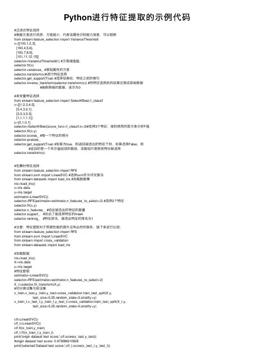
Python进⾏特征提取的⽰例代码#过滤式特征选择#根据⽅差进⾏选择,⽅差越⼩,代表该属性识别能⼒很差,可以剔除from sklearn.feature_selection import VarianceThresholdx=[[100,1,2,3],[100,4,5,6],[100,7,8,9],[101,11,12,13]]selector=VarianceThreshold(1) #⽅差阈值值,selector.fit(x)selector.variances_ #展现属性的⽅差selector.transform(x)#进⾏特征选择selector.get_support(True) #选择结果后,特征之前的索引selector.inverse_transform(selector.transform(x)) #将特征选择后的结果还原成原始数据#被剔除掉的数据,显⽰为0#单变量特征选择from sklearn.feature_selection import SelectKBest,f_classifx=[[1,2,3,4,5],[5,4,3,2,1],[3,3,3,3,3],[1,1,1,1,1]]y=[0,1,0,1]selector=SelectKBest(score_func=f_classif,k=3)#选择3个特征,指标使⽤的是⽅差分析F值selector.fit(x,y)selector.scores_ #每⼀个特征的得分selector.pvalues_selector.get_support(True) #如果为true,则返回被选出的特征下标,如果选择False,则#返回的是⼀个布尔值组成的数组,该数组只是那些特征被选择selector.transform(x)#包裹时特征选择from sklearn.feature_selection import RFEfrom sklearn.svm import LinearSVC #选择svm作为评定算法from sklearn.datasets import load_iris #加载数据集iris=load_iris()x=iris.datay=iris.targetestimator=LinearSVC()selector=RFE(estimator=estimator,n_features_to_select=2) #选择2个特征selector.fit(x,y)selector.n_features_ #给出被选出的特征的数量selector.support_ #给出了被选择特征的maskselector.ranking_ #特征排名,被选出特征的排名为1#注意:特征提取对于预测性能的提升没有必然的联系,接下来进⾏⽐较;from sklearn.feature_selection import RFEfrom sklearn.svm import LinearSVCfrom sklearn import cross_validationfrom sklearn.datasets import load_iris#加载数据iris=load_iris()X=iris.datay=iris.target#特征提取estimator=LinearSVC()selector=RFE(estimator=estimator,n_features_to_select=2)X_t=selector.fit_transform(X,y)#切分测试集与验证集x_train,x_test,y_train,y_test=cross_validation.train_test_split(X,y,test_size=0.25,random_state=0,stratify=y)x_train_t,x_test_t,y_train_t,y_test_t=cross_validation.train_test_split(X_t,y,test_size=0.25,random_state=0,stratify=y)clf=LinearSVC()clf_t=LinearSVC()clf.fit(x_train,y_train)clf_t.fit(x_train_t,y_train_t)print('origin dataset test score:',clf.score(x_test,y_test))#origin dataset test score: 0.973684210526print('selected Dataset:test score:',clf_t.score(x_test_t,y_test_t))#selected Dataset:test score: 0.947368421053import numpy as npfrom sklearn.feature_selection import RFECVfrom sklearn.svm import LinearSVCfrom sklearn.datasets import load_irisiris=load_iris()x=iris.datay=iris.targetestimator=LinearSVC()selector=RFECV(estimator=estimator,cv=3)selector.fit(x,y)selector.n_features_selector.support_selector.ranking_selector.grid_scores_#嵌⼊式特征选择import numpy as npfrom sklearn.feature_selection import SelectFromModelfrom sklearn.svm import LinearSVCfrom sklearn.datasets import load_digitsdigits=load_digits()x=digits.datay=digits.targetestimator=LinearSVC(penalty='l1',dual=False)selector=SelectFromModel(estimator=estimator,threshold='mean')selector.fit(x,y)selector.transform(x)selector.threshold_selector.get_support(indices=True)#scikitlearn提供了Pipeline来讲多个学习器组成流⽔线,通常流⽔线的形式为:将数据标准化,#--》特征提取的学习器————》执⾏预测的学习器,除了最后⼀个学习器之后,#前⾯的所有学习器必须提供transform⽅法,该⽅法⽤于数据转化(如归⼀化、正则化、#以及特征提取#学习器流⽔线(pipeline)from sklearn.svm import LinearSVCfrom sklearn.datasets import load_digitsfrom sklearn import cross_validationfrom sklearn.linear_model import LogisticRegressionfrom sklearn.pipeline import Pipelinedef test_Pipeline(data):x_train,x_test,y_train,y_test=datasteps=[('linear_svm',LinearSVC(C=1,penalty='l1',dual=False)),('logisticregression',LogisticRegression(C=1))]pipeline=Pipeline(steps)pipeline.fit(x_train,y_train)print('named steps',d_steps)print('pipeline score',pipeline.score(x_test,y_test))if __name__=='__main__':data=load_digits()x=data.datay=data.targettest_Pipeline(cross_validation.train_test_split(x,y,test_size=0.25,random_state=0,stratify=y))以上就是Python进⾏特征提取的⽰例代码的详细内容,更多关于Python 特征提取的资料请关注其它相关⽂章!。
一、介绍SIFT算法SIFT(Scale-Invariant Feature Transform)算法是一种用于图像处理和计算机视觉领域的特征提取算法,由David Lowe在1999年提出。
SIFT算法具有旋转、尺度、光照等方面的不变性,能够对图像进行稳健的特征点提取,被广泛应用于物体识别、图像匹配、图像拼接、三维重建等领域。
二、SIFT算法原理SIFT算法的主要原理包括尺度空间极值点检测、关键点定位、关键点方向确定、关键点描述等步骤。
其中,尺度空间极值点检测通过高斯差分金字塔来检测图像中的极值点,关键点定位则利用DoG响应函数进行关键点细化,关键点方向确定和关键点描述部分则通过梯度方向直方图和关键点周围区域的梯度幅度信息来完成。
三、使用Matlab实现SIFT算法在Matlab中实现SIFT算法,需要对SIFT算法的每个步骤进行详细的编程和调试。
需要编写代码进行图像的高斯金字塔和高斯差分金字塔的构建,计算尺度空间极值点,并进行关键点定位。
需要实现关键点的方向确定和描述子生成的算法。
将所有步骤整合在一起,完成SIFT算法的整体实现。
四、SIFT算法复杂代码的编写SIFT算法涉及到的步骤较多,需要编写复杂的代码来实现。
在编写SIFT算法的Matlab代码时,需要考虑到算法的高效性、可扩展性和稳定性。
具体来说,需要注意以下几点:1. 高斯差分金字塔和高斯金字塔的构建:在构建高斯差分金字塔时,需要编写代码实现图像的高斯滤波和图像的降采样操作,以得到不同尺度空间的图像。
还需要实现高斯差分金字塔的构建,以检测图像中的极值点。
2. 尺度空间极值点检测:在检测图像中的极值点时,需要编写代码实现对高斯差分金字塔的极值点检测算法,以找到图像中的潜在关键点。
3. 关键点的定位:关键点定位阶段需要编写代码实现对尺度空间极值点的精确定位,消除低对比度点和边缘响应点,并进行关键点的精细化操作。
4. 关键点的方向确定和描述子生成:在这一步骤中,需要编写代码实现对关键点周围区域的梯度幅度信息的计算和关键点方向的确定,以及生成关键点的描述子。
基于色标和尺度不变特征的实时特征提取方法徐斌;于乃功【摘要】With the background of mobile robot vision and with the aim of features required by monocular vision, a method for realtime feature extraction on the base of block of color and the Scale Invariant Feature Transform (SIFT) feature point operator is presented.The localization of feature includes color labeling location and feature points location. The color labeling location is aim to find the centre of gravity point of the color label from the scaling picture. The feature points location is on the base of color labeling {ocation, cuts a small image from the origin image, extracts the SIFT feature points of the object from the small image. The position of the tracked object are calculated by the max or min feature points, it provides foundation for the object tracking. The experimental results show it's effective.%以移动机器人视觉系统为背景,以单目视觉所需要的特征点为目标,提出一种基于颜色块和尺度不变特征点算子的实时特征提取方法;目标的定位分为色标定位和特征点定位两个过程,色标定位用来寻找在缩变图像上目标颜色块的重心点,特征点定位是在色标定位的基础上,切出小图像并提取目标的尺度不变特征点,根据极值特征点计算目标位置,为下一步的目标跟踪提供基础;实验结果验证了方法的有效性.【期刊名称】《计算机测量与控制》【年(卷),期】2011(019)002【总页数】4页(P409-411,414)【关键词】单目视觉;颜色块;目标跟踪;特征提取【作者】徐斌;于乃功【作者单位】北京工业大学,电子信息与控制工程学院,北京100124;华北科技学院机电工程系,河北,燕郊,101601;北京工业大学,电子信息与控制工程学院,北京100124【正文语种】中文【中图分类】TP3910 引言机器人视觉系统在机器人领域具有重要的作用。
dae特征提取代码DAE(Denoising Autoencoder)是一种用于无监督特征学习的深度学习模型,可以通过学习数据的表达来提取有用的特征。
DAE的主要思想是将输入数据加入噪声,然后用一个神经网络模型将加入噪声的数据重构为原始数据,通过最小化重构误差来训练模型。
以下是一个使用Python和TensorFlow实现DAE特征提取的代码示例:```pythonimport numpy as npimport tensorflow as tf#加载数据def load_data(:#加载数据的代码#定义DAE模型class DAE:def __init__(self, input_dim, hidden_dim, learning_rate):self.input_dim = input_dimself.hidden_dim = hidden_dimself.learning_rate = learning_rateself.build_modeldef build_model(self):#定义输入层self.inputs = tf.placeholder(tf.float32, [None,self.input_dim])#加入噪声noisy_inputs = self.inputs +tf.random_normal(tf.shape(self.inputs))#定义编码器self.encoder_weights =tf.Variable(tf.random_normal([self.input_dim, self.hidden_dim])) self.encoder_bias =tf.Variable(tf.random_normal([self.hidden_dim]))self.encoder_output = tf.nn.sigmoid(tf.matmul(noisy_inputs, self.encoder_weights) + self.encoder_bias)#定义解码器self.decoder_weights =tf.Variable(tf.random_normal([self.hidden_dim, self.input_dim])) self.decoder_bias =tf.Variable(tf.random_normal([self.input_dim]))self.decoder_output = tf.matmul(self.encoder_output,self.decoder_weights) + self.decoder_bias#定义损失函数self.loss = tf.reduce_mean(tf.square(self.inputs -self.decoder_output))#定义优化器self.optimizer =tf.train.AdamOptimizer(self.learning_rate).minimize(self.loss) def train(self, data, epochs, batch_size):with tf.Session( as sess:#初始化变量sess.run(tf.global_variables_initializer()#训练模型for epoch in range(epochs):np.random.shuffle(data)total_loss = 0for i in range(0, len(data), batch_size):batch = data[i:i+batch_size]_, loss = sess.run([self.optimizer, self.loss],feed_dict={self.inputs: batch})total_loss += lossavg_loss = total_loss / (len(data) // batch_size)print("Epoch:", epoch+1, "Loss:", avg_loss)#提取特征features = sess.run(self.encoder_output,feed_dict={self.inputs: data})return features#加载数据data = load_data#设置超参数input_dim = data.shape[1]hidden_dim = 100learning_rate = 0.001epochs = 100batch_size = 32#创建DAE模型dae = DAE(input_dim, hidden_dim, learning_rate)#训练模型并提取特征features = dae.train(data, epochs, batch_size)```上述代码中,首先定义了一个`load_data(`函数用于加载数据集,这里需要根据具体情况进行实现。

orb特征提取代码生成的标题:使用ORB算法实现图像特征提取使用ORB算法的图像特征提取在计算机视觉领域得到了广泛的应用。
ORB算法是一种基于FAST角点检测和BRIEF描述符的图像特征提取算法。
它具有旋转不变性和尺度不变性等特点,可以有效地解决图像匹配和物体跟踪等问题。
下面我们就来一步步讲解使用ORB算法进行图像特征提取的详细过程。
首先,我们需要导入OpenCV库和NumPy库,在Python中使用以下代码即可完成:```pythonimport cv2import numpy as np```接着,我们可以定义一个函数,来读取并显示图像文件,代码如下:```pythondef show_image(img_file):img = cv2.imread(img_file)cv2.imshow("image", img)cv2.waitKey(0)cv2.destroyAllWindows()```在显示图像的同时,我们也可以使用ORB算法提取图像的特征点和描述符。
ORB算法基于FAST角点检测和BRIEF描述符,可以有效地提取图像的特征信息。
下面是使用ORB算法提取特征点和描述符的代码:```pythondef extract_ORB_feature(img_file):img = cv2.imread(img_file)gray = cv2.cvtColor(img, cv2.COLOR_BGR2GRAY)orb = cv2.ORB_create()keypoints, descriptors = orb.detectAndCompute(gray, None)print("Number of keypoints detected: ",len(keypoints))return keypoints, descriptors```该函数会返回ORB算法提取出的关键点(keypoints)和描述符(descriptors)。
尺度不变特征变换算法一、前言尺度不变特征变换算法(Scale-Invariant Feature Transform,SIFT)是一种用于图像处理和计算机视觉的算法,由David Lowe于1999年提出。
SIFT算法可以在不同尺度和旋转下找到图像中的关键点,并提取出这些关键点的局部特征描述符,从而实现对图像的匹配、识别等任务。
二、SIFT算法原理1. 尺度空间构建SIFT算法首先通过高斯滤波器构建尺度空间,以便在不同尺度下检测图像中的关键点。
高斯滤波器可以模拟人眼对图像的模糊效果,使得在不同尺度下能够检测到具有相似形状但大小不同的物体。
2. 关键点检测在构建好尺度空间后,SIFT算法通过DoG(差分高斯)金字塔来寻找关键点。
DoG金字塔是由相邻两层高斯金字塔之差得到的,它可以有效地检测出具有不同尺度和方向的局部极值点。
3. 方向分配为了使得特征描述子具有旋转不变性,在确定关键点位置后,SIFT算法还需要计算每个关键点的主方向。
它通过计算关键点周围像素的梯度方向直方图来确定主方向,从而使得特征描述子能够在不同角度下进行匹配。
4. 特征描述在确定了关键点位置和主方向之后,SIFT算法通过计算关键点周围像素的梯度幅值和方向来生成特征描述子。
这个过程中,SIFT算法使用了一个16×16的窗口,并将其分成4×4个小窗口,在每个小窗口中计算8个梯度方向的直方图,最终生成一个128维的特征向量。
5. 特征匹配在提取出两幅图像中所有关键点的特征描述子后,SIFT算法采用欧氏距离来计算两个特征向量之间的相似度,并使用比率测试来判断是否为匹配点。
如果两个特征向量之间的距离小于一定阈值,并且与次近邻之间距离比例大于一定比例,则认为是匹配点。
三、SIFT算法优缺点1. 优点:(1)尺度不变性:SIFT算法可以在不同尺度下检测到具有相似形状但大小不同的物体;(2)旋转不变性:SIFT算法可以计算每个关键点的主方向,从而使得特征描述子能够在不同角度下进行匹配;(3)鲁棒性:SIFT算法对于光照、视角、噪声等因素有较好的鲁棒性。
OPENCV特征提取代码总结OpenCV是一个计算机视觉库,提供了许多用于图像处理和计算机视觉任务的函数和算法。
其中特征提取是OpenCV中一个非常重要的功能,它可以从图像中提取出能够表达图像特征的向量。
下面是几个常见的特征提取方法的代码总结。
1. Harris角点检测算法代码Harris角点检测算法是一种常用的角点检测算法,可以检测图像中的角点。
它的代码如下:```import cv2import numpy as npdef harris_corner_detector(image):gray = cv2.cvtColor(image, cv2.COLOR_BGR2GRAY)#计算图像的梯度dx = cv2.Sobel(gray, cv2.CV_64F, 1, 0, ksize=3)dy = cv2.Sobel(gray, cv2.CV_64F, 0, 1, ksize=3)# 计算Harris角点响应函数dx2 = cv2.multiply(dx, dx)dy2 = cv2.multiply(dy, dy)dxy = cv2.multiply(dx, dy)k=0.04det = cv2.subtract(cv2.multiply(dx2, dy2), cv2.multiply(dxy, dxy))trace = cv2.add(dx2, dy2)response = cv2.divide(det, trace + k)#寻找响应值大于阈值的角点corners = []threshold = 0.01for i in range(response.shape[0]):for j in range(response.shape[1]):if response[i, j] > threshold:corners.append(cv2.KeyPoint(j, i, 1, -1, response[i, j]))return corners# 调用Harris角点检测算法image = cv2.imread('image.jpg')corners = harris_corner_detector(image)#在图片上绘制出检测到的角点cv2.drawKeypoints(image, corners, image)cv2.imshow('image', image)cv2.waitKey(0)cv2.destroyAllWindows```2.SIFT特征提取算法代码SIFT(Scale-Invariant Feature Transform)是一种尺度不变的特征提取算法,可以提取出图像的关键点和对应的描述子。
特征提取模型代码特征提取是机器学习中非常重要的一个环节,通常特征提取模型代码是实现特征提取的核心代码。
在本文中,我们将分步骤地讨论特征提取模型代码,以便更好地理解这个过程。
1. 导入必要的库在开始编写特征提取代码之前,我们需要导入一些必要的库。
根据不同的任务和需要,导入的库可能有所不同。
但是,通常情况下,我们需要导入numpy、pandas、scikit-learn等库。
```pythonimport numpy as npimport pandas as pdfrom sklearn.feature_extraction.text import CountVectorizer, TfidfVectorizer```2. 加载数据特征提取的第一步是加载数据。
在加载数据时,我们需要指定文件路径或URL或者其他可以获取数据的方式。
然后,将数据转换为特定格式的数据框或张量,以便在后续步骤中使用。
```pythondata = pd.read_csv("data.csv")X = data["text"].valuesy = data["label"].values```3. 特征提取特征提取是特征工程的核心步骤之一。
它的主要目的是从原始数据中提取有意义的特征。
这些特征可以是文本中的单词或短语、图像中的纹理或颜色、声音中的频率模式等。
下面是在文本数据上使用CountVectorizer和TfidfVectorizer进行特征提取的示例代码。
```python# CountVectorizercv = CountVectorizer()X_cv = cv.fit_transform(X)# TfidfVectorizertfidf = TfidfVectorizer()X_tfidf = tfidf.fit_transform(X)```4. 特征选择在进行特征提取之后,我们需要对提取出的特征进行选择。
hog特征提取代码
hog特征提取是一种用于图像处理和计算机视觉中的特征提取方法,它可以提取出图像中的纹理、边缘和形状等特征,具有很好的鉴别能力和抗干扰性。
以下是hog特征提取代码示例:
1. 导入必要的库和模块
import cv2
import numpy as np
from skimage.feature import hog
2. 读取图像
img = cv2.imread('test.jpg', cv2.COLOR_BGR2GRAY)
3. 计算hog特征
fd, hog_image = hog(img, orientations=8,
pixels_per_cell=(16, 16), cells_per_block=(1, 1),
visualize=True, multichannel=False)
其中,orientations参数表示方向数,pixels_per_cell参数表示每个cell的像素大小,cells_per_block参数表示每个block的cell数量,multichannel参数表示是否为多通道图像。
4. 显示hog特征图像
cv2.imshow('HOG Image', hog_image)
cv2.waitKey(0)
cv2.destroyAllWindows()
以上就是简单的hog特征提取代码示例,可以根据具体需求进行
参数调整和优化。
多尺度特征提取代码特征提取是计算机视觉和图像处理中的重要任务,它可以帮助我们理解图像中的信息并进行后续的分析和识别。
在这里,我将从多个角度介绍特征提取的代码实现。
首先,特征提取的方法有很多种,比如SIFT、SURF、HOG、LBP 等。
这些方法都有对应的开源库或者工具包,比如OpenCV、Scikit-image、Dlib等。
你可以根据你的需求选择合适的方法和工具。
以OpenCV为例,以下是一个简单的多尺度特征提取的代码示例:python.import cv2。
# 读取图像。
image = cv2.imread('image.jpg')。
# 转换为灰度图像。
gray = cv2.cvtColor(image, cv2.COLOR_BGR2GRAY)。
# 初始化SIFT检测器。
sift = cv2.SIFT_create()。
# 检测关键点和计算描述符。
keypoints, descriptors = sift.detectAndCompute(gray, None)。
# 绘制关键点。
image_with_keypoints = cv2.drawKeypoints(image, keypoints, None)。
# 显示结果。
cv2.imshow('Image with Keypoints',image_with_keypoints)。
cv2.waitKey(0)。
cv2.destroyAllWindows()。
上面的代码演示了如何使用OpenCV中的SIFT算法进行多尺度特征提取。
首先读取图像,然后将其转换为灰度图像。
接着初始化SIFT检测器,检测关键点并计算描述符,最后绘制关键点并显示结果。
除了SIFT之外,还可以使用其他特征提取方法,比如SURF、HOG等。
它们的使用方式也类似,只是需要调用对应的函数和参数。
另外,如果你使用的是Python,还可以使用Scikit-image库进行特征提取。
视觉SLAM⼗四讲——特征提取和匹配主要内容1. 常⽤的特征提取的⽅法:SIFT SURF ORB 其中,SIFT(尺度不变特征变换,Scale-Invariant Feature Transform)最为经典,充分考虑了相机的运动,光照变化,以及尺度和旋转变化,但需要较⼤的计算量, 在普通pc cpu上⽆法实时计算SIFT特征进⾏定位与建图 考虑适当减低精度和健壮性,减⼩计算量,如下两种: FAST关键点:没有描述⼦ ORB (Oriented FAST and Rotated BRIEF): 改进了FAST检测⼦不具有⽅向性的问题,并采⽤速度极快的⼆进制描述⼦BRIEF。
2. ORB特征——FAST关键点 1)选取周围半径为3的圆上的像素点,检测连续超过本像素点正负p%门限的像素点个数,根据个数分别为FAST-9, FAST-11, FAST-12。
2)预处理,排除⾮⾓点像素,增加处理速度 3)避免⾓点集中,采⽤⾮极⼤值抑制,在⼀定区域仅保留响应极⼤值的⾓点 4)提取最终的⾓点数量N,选取前N个最⼤响应值5)尺度不变性:构建图像⾦字塔 6)旋转:灰度质⼼法3. ORB特征——BRIEF描述⼦ 4. 特征匹配 计算所有特征点描述⼦距离,表征了特征点的相似程度 (采⽤不同的距离度量范数,浮点型描述⼦-欧⽒距离,⼆进制描述⼦-汉明距离) 匹配算法: 快速近似最近邻(FLANN)5. 正确匹配筛选的依据:汉明距离⼩于最⼩距离的两倍,⼯程上的经验⽅法 在后⾯的运动估计中,还需要使⽤去除误匹配的算法参考链接代码#include <iostream>#include <opencv2/core/core.hpp>#include <opencv2/features2d/features2d.hpp>#include <opencv2/highgui/highgui.hpp>using namespace std;using namespace cv;int main ( int argc, char** argv ){if ( argc != 3 ){cout<<"usage: feature_extraction img1 img2"<<endl;return1;}//-- 读取图像Mat img_1 = imread ( argv[1], CV_LOAD_IMAGE_COLOR );Mat img_2 = imread ( argv[2], CV_LOAD_IMAGE_COLOR );//-- 初始化std::vector<KeyPoint> keypoints_1, keypoints_2;Mat descriptors_1, descriptors_2;Ptr<FeatureDetector> detector = ORB::create();Ptr<DescriptorExtractor> descriptor = ORB::create();// Ptr<FeatureDetector> detector = FeatureDetector::create(detector_name);// Ptr<DescriptorExtractor> descriptor = DescriptorExtractor::create(descriptor_name);Ptr<DescriptorMatcher> matcher = DescriptorMatcher::create ( "BruteForce-Hamming" );//-- 第⼀步:检测 Oriented FAST ⾓点位置detector->detect ( img_1,keypoints_1 );detector->detect ( img_2,keypoints_2 );//-- 第⼆步:根据⾓点位置计算 BRIEF 描述⼦descriptor->compute ( img_1, keypoints_1, descriptors_1 );descriptor->compute ( img_2, keypoints_2, descriptors_2 );Mat outimg1;drawKeypoints( img_1, keypoints_1, outimg1, Scalar::all(-1), DrawMatchesFlags::DEFAULT );imshow("ORB特征点",outimg1); imwrite ("ORB_Feature.png", outimg1);//-- 第三步:对两幅图像中的BRIEF描述⼦进⾏匹配,使⽤ Hamming 距离vector<DMatch> matches;//BFMatcher matcher ( NORM_HAMMING );matcher->match ( descriptors_1, descriptors_2, matches );//-- 第四步:匹配点对筛选double min_dist=10000, max_dist=0;//找出所有匹配之间的最⼩距离和最⼤距离, 即是最相似的和最不相似的两组点之间的距离for ( int i = 0; i < descriptors_1.rows; i++ ){double dist = matches[i].distance;if ( dist < min_dist ) min_dist = dist;if ( dist > max_dist ) max_dist = dist;}// 仅供娱乐的写法min_dist = min_element( matches.begin(), matches.end(), [](const DMatch& m1, const DMatch& m2) {return m1.distance<m2.distance;} )->distance; max_dist = max_element( matches.begin(), matches.end(), [](const DMatch& m1, const DMatch& m2) {return m1.distance<m2.distance;} )->distance; printf ( "-- Max dist : %f \n", max_dist );printf ( "-- Min dist : %f \n", min_dist );//当描述⼦之间的距离⼤于两倍的最⼩距离时,即认为匹配有误.但有时候最⼩距离会⾮常⼩,设置⼀个经验值30作为下限.std::vector< DMatch > good_matches;for ( int i = 0; i < descriptors_1.rows; i++ ){if ( matches[i].distance <= max ( 2*min_dist, 30.0 ) ){good_matches.push_back ( matches[i] );}}//-- 第五步:绘制匹配结果Mat img_match;Mat img_goodmatch;drawMatches ( img_1, keypoints_1, img_2, keypoints_2, matches, img_match );drawMatches ( img_1, keypoints_1, img_2, keypoints_2, good_matches, img_goodmatch );imshow ( "所有匹配点对", img_match );imshow ( "优化后匹配点对", img_goodmatch ); // 保存图像imwrite ("all_feature_matching.png", img_match);imwrite ("good_feature_matching.png", img_goodmatch);waitKey(0);return0;}结果输出。
一、介绍SIFT特征提取算法SIFT(Scale-Invariant Feature Transform)是一种用于图像处理和计算机视觉领域的特征提取算法,由David Lowe在1999年提出。
SIFT算法能够在不同尺度、旋转和光照条件下检测和描述图像中的关键特征点。
二、SIFT特征提取的原理1. 尺度空间极值检测SIFT算法首先通过高斯滤波器构建图像的尺度空间金字塔,在不同尺度上检测图像中的极值点,用于定位关键特征点。
2. 关键点定位在尺度空间金字塔上定位极值点,并通过尺度空间的拟合插值定位关键点的位置和尺度。
3. 方向确定对关键点周围的梯度方向进行统计,选择主要梯度方向作为关键点的方向。
4. 关键点描述基于关键点周围的梯度幅值和方向构建特征向量,用于描述关键点的外观特征。
三、MATLAB实现SIFT特征提取代码MATLAB提供了丰富的图像处理工具包,其中也包括对SIFT算法的支持。
下面给出MATLAB实现SIFT特征提取的简单示例代码:```matlab读入图像I = imread('image.jpg');I = single(rgb2gray(I));提取SIFT特征点[f, d] = vl_sift(I);显示特征点imshow(I);h1 = vl_plotframe(f);h2 = vl_plotsiftdescriptor(d, f);set(h1,'color','k','linewidth',3);set(h2,'color','g');```上述代码中,首先使用`imread`读入一张图像,并将其转化为灰度图像。
然后使用`vl_sift`函数提取图像中的SIFT特征点,其中`f`为特征点的位置和尺度,`d`为特征点的描述子。
最后使用`vl_plotframe`和`vl_plotsiftdescriptor`函数将特征点和特征描述子可视化出来。
图像特征提取的代码实现技巧图像特征提取是计算机视觉领域的一项基础任务。
通过提取图像中的关键特征,可以帮助计算机理解和分析图像,从而实现图像分类、目标检测、图像检索等应用。
本文将介绍图像特征提取的一些常见方法和实现技巧。
一、常见的图像特征描述方法1. SIFT (尺度不变特征转换)SIFT特征是一种基于尺度空间的特征描述子,具有尺度不变性和旋转不变性。
其基本流程包括尺度空间构建、关键点提取、关键点精确定位、关键点方向计算和关键点描述子生成等步骤。
2. SURF (加速稳健特征)SURF特征是对SIFT特征的一种改进,通过使用积分图像和快速Harris角点检测等方法,加快了特征提取的速度。
SURF特征也具有尺度不变性和旋转不变性。
3. ORB (Oriented FAST and Rotated BRIEF)ORB特征是一种二进制局部特征描述子,结合了FAST角点检测和BRIEF特征描述子。
ORB特征具有快速提取速度和良好的旋转不变性。
4. HOG (方向梯度直方图)HOG特征是一种基于图像梯度信息的特征描述子,通过计算图像中不同方向上的梯度直方图,来描述图像的纹理和形状特征。
HOG特征在目标检测和行人识别等任务中得到广泛应用。
5. LBP (局部二值模式)LBP特征是一种用来描述图像局部纹理特征的方法,通过比较图像中像素与其邻域像素的灰度值大小关系,将局部纹理模式编码为二进制数。
LBP特征在人脸识别、纹理分类等任务中具有较好的性能。
二、图像特征提取的实现技巧1.特征提取的图像预处理在进行特征提取之前,通常需要对原始图像进行预处理,以提高特征提取的效果。
例如,可以对图像进行灰度化、归一化、降噪等操作。
2.特征提取的关键点选择在进行特征提取时,需要选择合适的关键点进行特征计算,以保证提取到的特征具有代表性。
通常可以使用角点检测方法(如Harris 角点检测、FAST角点检测)来选择关键点。
3.特征描述子的生成和匹配特征描述子是用来描述关键点周围图像局部特征的向量表示。
dae特征提取代码清华大学开源的数据增强库DAE(Data Augmentation for End-to-end Speech Recognition)提供了用于语音识别任务的数据增强相关功能。
该库基于Kaldi,旨在提高语音识别模型在多样性和变化性方面的鲁棒性。
特征提取是语音识别任务中的重要步骤之一,它将原始的语音信号转化为一种更易于模型处理的表示形式。
下面是DAE库中提供的特征提取代码的示例。
```pythonimport numpy as npimport librosafrom dae.data_augmentation import SpecAugment#定义特征提取函数def extract_features(audio_path):#加载音频文件audio, sr = librosa.load(audio_path, sr=None)#提取语谱图特征spectrogram = librosa.stft(audio)spectrogram = np.abs(spectrogram)#应用数据增强augmented_spectrogram = augmenter.augment(spectrogram)#将语谱图特征转换为对数刻度log_spectrogram =librosa.amplitude_to_db(augmented_spectrogram, ref=np.max) #归一化处理normalized_spectrogram = (log_spectrogram -np.mean(log_spectrogram)) / np.std(log_spectrogram)#返回特征return normalized_spectrogram```请注意,上述代码只是DAE库中特征提取的一个示例,实际的特征提取过程可能因任务需求而有所调整。
对于语音识别任务,还可以考虑其他特征,如梅尔频谱倒谱系数(MFCC)等。
function [ pos, scale, orient, desc ] = SIFT( im, octaves, intervals, object_mask, contrast_threshold, curvature_threshold, interactive )% 功能:提取灰度图像的尺度不变特征(SIFT特征)% 输入:% im - 灰度图像,该图像的灰度值在0到1之间(注意:应首先对输入图像的灰度值进行归一化处理)% octaves - 金字塔的组数:octaves (默认值为4).% intervals - 该输入参数决定每组金字塔的层数(默认值为2).% object_mask - 确定图像中尺度不变特征点的搜索区域,如果没有特别指出,则算法将搜索整个图像% contrast_threshold - 对比度阈值(默认值为0.03).% curvature_threshold - 曲率阈值(默认值为10.0).% interactive - 函数运行显示标志,将其设定为1,则显示算法运行时间和过程的相关信息;% 如果将其设定为2,则仅显示最终运行记过(default = 1).% 输出:% pos - Nx2 矩阵,每一行包括尺度不变特征点的坐标(x,y)% scale - Nx3 矩阵,每一行包括尺度不变特征点的尺度信息(第一列是尺度不变特征点所在的组,% 第二列是其所在的层, 第三列是尺度不变特征点的sigma).% orient - Nx1 向量,每个元素是特征点的主方向,其范围在[-pi,pi)之间.% desc - Nx128 矩阵,每一行包含特征点的特征向量.% 参考文献:% [1] David G. Lowe, "Distinctive Image Features from Sacle-Invariant Keypoints",% accepted for publicatoin in the International Journal of Computer% Vision, 2004.% [2] David G. Lowe, "Object Recognition from Local Scale-Invariant Features",% Proc. of the International Conference on Computer Vision, Corfu,% September 1999.%% Xiaochuan ZHAO;zhaoxch@% 设定输入量的默认值if ~exist('octaves')octaves = 4;endif ~exist('intervals')intervals = 2;endif ~exist('object_mask')object_mask = ones(size(im));endif size(object_mask) ~= size(im)object_mask = ones(size(im));endif ~exist('contrast_threshold')contrast_threshold = 0.02; %0.03吧endif ~exist('curvature_threshold')curvature_threshold = 10.0;endif ~exist('interactive')interactive = 1;end% 检验输入灰度图像的像素灰度值是否已归一化到[0,1]if( (min(im(:)) < 0) | (max(im(:)) > 1) )fprintf( 2, 'Warning: image not normalized to [0,1].\n' );end% 将输入图像经过高斯平滑处理,采用双线性差值将其扩大一倍.if interactive >= 1fprintf( 2, 'Doubling image size for first octave...\n' );endtic;antialias_sigma = 0.5;if antialias_sigma == 0signal = im;elseg = gaussian_filter( antialias_sigma );if exist('corrsep') == 3signal = corrsep( g, g, im );elsesignal = conv2( g, g, im, 'same' );endendsignal = im;[X Y] = meshgrid( 1:0.5:size(signal,2), 1:0.5:size(signal,1) );signal = interp2( signal, X, Y, '*linear' );subsample = [0.5]; % 降采样率;%下一步是生成高斯和差分高斯(DOG)金字塔,这两个金字塔的数据分别存储在名为gauss_pyr{orient,interval}% 和DOG_pyr{orient,interval}的元胞数字中。
高斯金字塔含有s+3层,差分高斯金字塔含有s+2层。
if interactive >= 1fprintf( 2, 'Prebluring image...\n' );endpreblur_sigma = sqrt(sqrt(2)^2 - (2*antialias_sigma)^2);if preblur_sigma == 0gauss_pyr{1,1} = signal;elseg = gaussian_filter( preblur_sigma );if exist('corrsep') == 3gauss_pyr{1,1} = corrsep( g, g, signal );elsegauss_pyr{1,1} = conv2( g, g, signal, 'same' );endendclear signalpre_time = toc;if interactive >= 1fprintf( 2, 'Preprocessing time %.2f seconds.\n', pre_time );end% 第一组第一层的sigmainitial_sigma = sqrt( (2*antialias_sigma)^2 + preblur_sigma^2 );% 记录每一层和每一个尺度的sigmaabsolute_sigma = zeros(octaves,intervals+3);absolute_sigma(1,1) = initial_sigma * subsample(1);% 记录产生金字塔的滤波器的尺寸和标准差filter_size = zeros(octaves,intervals+3);filter_sigma = zeros(octaves,intervals+3);% 生成高斯和差分高斯金字塔if interactive >= 1fprintf( 2, 'Expanding the Gaussian and DOG pyramids...\n' );endtic;for octave = 1:octavesif interactive >= 1fprintf( 2, '\tProcessing octave %d: image size %d x %d subsample %.1f\n', octave,size(gauss_pyr{octave,1},2), size(gauss_pyr{octave,1},1), subsample(octave) );fprintf( 2, '\t\tInterval 1 sigma %f\n', absolute_sigma(octave,1) );endsigma = initial_sigma;g = gaussian_filter( sigma );filter_size( octave, 1 ) = length(g);filter_sigma( octave, 1 ) = sigma;DOG_pyr{octave} = zeros(size(gauss_pyr{octave,1},1),size(gauss_pyr{octave,1},2),intervals+2);for interval = 2:(intervals+3)% 计算生成下一层几何采样金字塔的标准差% 其中,sigma_i+1 = k*sigma.% sigma_i+1^2 = sigma_f,i^2 + sigma_i^2% (k*sigma_i)^2 = sigma_f,i^2 + sigma_i^2% 因此:% sigma_f,i = sqrt(k^2 - 1)sigma_i% 对于扩展的组(span the octave),k = 2^(1/intervals)% 所以% sigma_f,i = sqrt(2^(2/intervals) - 1)sigma_isigma_f = sqrt(2^(2/intervals) - 1)*sigma;g = gaussian_filter( sigma_f );sigma = (2^(1/intervals))*sigma;% 记录sigma的值absolute_sigma(octave,interval) = sigma * subsample(octave);% 记录滤波器的尺寸和标准差filter_size(octave,interval) = length(g);filter_sigma(octave,interval) = sigma;if exist('corrsep') == 3gauss_pyr{octave,interval} = corrsep( g, g, gauss_pyr{octave,interval-1} );elsegauss_pyr{octave,interval} = conv2( g, g, gauss_pyr{octave,interval-1}, 'same' );endDOG_pyr{octave}(:,:,interval-1) = gauss_pyr{octave,interval} - gauss_pyr{octave,interval-1};if interactive >= 1fprintf( 2, '\t\tInterval %d sigma %f\n', interval, absolute_sigma(octave,interval) );endendif octave < octavessz = size(gauss_pyr{octave,intervals+1});[X Y] = meshgrid( 1:2:sz(2), 1:2:sz(1) );gauss_pyr{octave+1,1} = interp2(gauss_pyr{octave,intervals+1},X,Y,'*nearest');absolute_sigma(octave+1,1) = absolute_sigma(octave,intervals+1);subsample = [subsample subsample(end)*2];endendpyr_time = toc;if interactive >= 1fprintf( 2, 'Pryamid processing time %.2f seconds.\n', pyr_time );end% 在交互模式下显示高斯金字塔if interactive >= 2sz = zeros(1,2);sz(2) = (intervals+3)*size(gauss_pyr{1,1},2);for octave = 1:octavessz(1) = sz(1) + size(gauss_pyr{octave,1},1);endpic = zeros(sz);y = 1;for octave = 1:octavesx = 1;sz = size(gauss_pyr{octave,1});for interval = 1:(intervals + 3)pic(y:(y+sz(1)-1),x:(x+sz(2)-1)) = gauss_pyr{octave,interval};x = x + sz(2);endy = y + sz(1);endfig = figure;clf;imshow(pic);resizeImageFig( fig, size(pic), 0.25 );fprintf( 2, 'The gaussian pyramid (0.25 scale).\nPress any key to continue.\n' );pause;close(fig)end% 在交互模式下显示差分高斯金字塔if interactive >= 2sz = zeros(1,2);sz(2) = (intervals+2)*size(DOG_pyr{1}(:,:,1),2);for octave = 1:octavessz(1) = sz(1) + size(DOG_pyr{octave}(:,:,1),1);endpic = zeros(sz);y = 1;for octave = 1:octavesx = 1;sz = size(DOG_pyr{octave}(:,:,1));for interval = 1:(intervals + 2)pic(y:(y+sz(1)-1),x:(x+sz(2)-1)) = DOG_pyr{octave}(:,:,interval);x = x + sz(2);endy = y + sz(1);endfig = figure;clf;imagesc(pic);resizeImageFig( fig, size(pic), 0.25 );fprintf( 2, 'The DOG pyramid (0.25 scale).\nPress any key to continue.\n' );pause;close(fig)end% 下一步是查找差分高斯金字塔中的局部极值,并通过曲率和照度进行检验curvature_threshold = ((curvature_threshold + 1)^2)/curvature_threshold;% 二阶微分核xx = [ 1 -2 1 ];yy = xx';xy = [ 1 0 -1; 0 0 0; -1 0 1 ]/4;raw_keypoints = [];contrast_keypoints = [];curve_keypoints = [];% 在高斯金字塔中查找局部极值if interactive >= 1fprintf( 2, 'Locating keypoints...\n' );endtic;loc = cell(size(DOG_pyr));for octave = 1:octavesif interactive >= 1fprintf( 2, '\tProcessing octave %d\n', octave );endfor interval = 2:(intervals+1)keypoint_count = 0;contrast_mask = abs(DOG_pyr{octave}(:,:,interval)) >= contrast_threshold;loc{octave,interval} = zeros(size(DOG_pyr{octave}(:,:,interval)));if exist('corrsep') == 3edge = 1;elseedge = ceil(filter_size(octave,interval)/2);endfor y=(1+edge):(size(DOG_pyr{octave}(:,:,interval),1)-edge)for x=(1+edge):(size(DOG_pyr{octave}(:,:,interval),2)-edge)if object_mask(round(y*subsample(octave)),round(x*subsample(octave))) == 1 if( (interactive >= 2) | (contrast_mask(y,x) == 1) )% 通过空间核尺度检测最大值和最小值tmp = DOG_pyr{octave}((y-1):(y+1),(x-1):(x+1),(interval-1):(interval+1));pt_val = tmp(2,2,2);if( (pt_val == min(tmp(:))) | (pt_val == max(tmp(:))) )% 存储对灰度大于对比度阈值的点的坐标raw_keypoints = [raw_keypoints; x*subsample(octave) y*subsample(octave)];if abs(DOG_pyr{octave}(y,x,interval)) >= contrast_thresholdcontrast_keypoints = [contrast_keypoints; raw_keypoints(end,:)];% 计算局部极值的Hessian矩阵Dxx = sum(DOG_pyr{octave}(y,x-1:x+1,interval) .* xx);Dyy = sum(DOG_pyr{octave}(y-1:y+1,x,interval) .* yy);Dxy = sum(sum(DOG_pyr{octave}(y-1:y+1,x-1:x+1,interval) .* xy));% 计算Hessian矩阵的直迹和行列式.Tr_H = Dxx + Dyy;Det_H = Dxx*Dyy - Dxy^2;% 计算主曲率.curvature_ratio = (Tr_H^2)/Det_H;if ((Det_H >= 0) & (curvature_ratio < curvature_threshold))% 存储主曲率小于阈值的的极值点的坐标(非边缘点)curve_keypoints = [curve_keypoints; raw_keypoints(end,:)];% 将该点的位置的坐标设为1,并计算点的数量.loc{octave,interval}(y,x) = 1;keypoint_count = keypoint_count + 1;endendendendendendendif interactive >= 1fprintf( 2, '\t\t%d keypoints found on interval %d\n', keypoint_count, interval );endendendkeypoint_time = toc;if interactive >= 1fprintf( 2, 'Keypoint location time %.2f seconds.\n', keypoint_time );end% 在交互模式下显示特征点检测的结果.if interactive >= 2fig = figure;clf;imshow(im);hold on;plot(raw_keypoints(:,1),raw_keypoints(:,2),'y+');resizeImageFig( fig, size(im), 2 );fprintf( 2, 'DOG extrema (2x scale).\nPress any key to continue.\n' );pause;close(fig);fig = figure;clf;imshow(im);hold on;plot(contrast_keypoints(:,1),contrast_keypoints(:,2),'y+');resizeImageFig( fig, size(im), 2 );fprintf( 2, 'Keypoints after removing low contrast extrema (2x scale).\nPress any key to continue.\n' );pause;close(fig);fig = figure;clf;imshow(im);hold on;plot(curve_keypoints(:,1),curve_keypoints(:,2),'y+');resizeImageFig( fig, size(im), 2 );fprintf( 2, 'Keypoints after removing edge points using principal curvature filtering (2x scale).\nPress any key to continue.\n' );pause;close(fig);endclear raw_keypoints contrast_keypoints curve_keypoints% 下一步是计算特征点的主方向.% 在特征点的一个区域内计算其梯度直方图g = gaussian_filter( 1.5 * absolute_sigma(1,intervals+3) / subsample(1) );zero_pad = ceil( length(g) / 2 );% 计算高斯金字塔图像的梯度方向和幅值if interactive >= 1fprintf( 2, 'Computing gradient magnitude and orientation...\n' );endtic;mag_thresh = zeros(size(gauss_pyr));mag_pyr = cell(size(gauss_pyr));grad_pyr = cell(size(gauss_pyr));for octave = 1:octavesfor interval = 2:(intervals+1)% 计算x,y的差分diff_x = 0.5*(gauss_pyr{octave,interval}(2:(end-1),3:(end))-gauss_pyr{octave,interval}(2:(end-1),1:(end-2 )));diff_y = 0.5*(gauss_pyr{octave,interval}(3:(end),2:(end-1))-gauss_pyr{octave,interval}(1:(end-2),2:(end-1 )));% 计算梯度幅值mag = zeros(size(gauss_pyr{octave,interval}));mag(2:(end-1),2:(end-1)) = sqrt( diff_x .^ 2 + diff_y .^ 2 );% 存储高斯金字塔梯度幅值mag_pyr{octave,interval} = zeros(size(mag)+2*zero_pad);mag_pyr{octave,interval}((zero_pad+1):(end-zero_pad),(zero_pad+1):(end-zero_pad)) = mag;% 计算梯度主方向grad = zeros(size(gauss_pyr{octave,interval}));grad(2:(end-1),2:(end-1)) = atan2( diff_y, diff_x );grad(find(grad == pi)) = -pi;% 存储高斯金字塔梯度主方向grad_pyr{octave,interval} = zeros(size(grad)+2*zero_pad);grad_pyr{octave,interval}((zero_pad+1):(end-zero_pad),(zero_pad+1):(end-zero_pad)) = grad;endendclear mag gradgrad_time = toc;if interactive >= 1fprintf( 2, 'Gradient calculation time %.2f seconds.\n', grad_time );end% 下一步是确定特征点的主方向% 方法:通过寻找每个关键点的子区域内梯度直方图的峰值(注:每个关键点的主方向可以有不止一个)% 将灰度直方图分为36等分,每隔10度一份num_bins = 36;hist_step = 2*pi/num_bins;hist_orient = [-pi:hist_step:(pi-hist_step)];% 初始化关键点的位置、方向和尺度信息pos = [];orient = [];scale = [];% 给关键点确定主方向if interactive >= 1fprintf( 2, 'Assigining keypoint orientations...\n' );endtic;for octave = 1:octavesif interactive >= 1fprintf( 2, '\tProcessing octave %d\n', octave );endfor interval = 2:(intervals + 1)if interactive >= 1fprintf( 2, '\t\tProcessing interval %d ', interval );endkeypoint_count = 0;% 构造高斯加权掩模g = gaussian_filter( 1.5 * absolute_sigma(octave,interval)/subsample(octave) );hf_sz = floor(length(g)/2);g = g'*g;loc_pad = zeros(size(loc{octave,interval})+2*zero_pad);loc_pad((zero_pad+1):(end-zero_pad),(zero_pad+1):(end-zero_pad)) = loc{octave,interval};[iy ix]=find(loc_pad==1);for k = 1:length(iy)x = ix(k);y = iy(k);wght = g.*mag_pyr{octave,interval}((y-hf_sz):(y+hf_sz),(x-hf_sz):(x+hf_sz));grad_window = grad_pyr{octave,interval}((y-hf_sz):(y+hf_sz),(x-hf_sz):(x+hf_sz));orient_hist=zeros(length(hist_orient),1);for bin=1:length(hist_orient)diff = mod( grad_window - hist_orient(bin) + pi, 2*pi ) - pi;orient_hist(bin)=orient_hist(bin)+sum(sum(wght.*max(1 - abs(diff)/hist_step,0)));end% 运用非极大抑制法查找主方向直方图的峰值peaks = orient_hist;rot_right = [ peaks(end); peaks(1:end-1) ];rot_left = [ peaks(2:end); peaks(1) ];peaks( find(peaks < rot_right) ) = 0;peaks( find(peaks < rot_left) ) = 0;% 提取最大峰值的值和其索引位置[max_peak_val ipeak] = max(peaks);% 将大于等于最大峰值80% 的直方图的也确定为特征点的主方向peak_val = max_peak_val;while( peak_val > 0.8*max_peak_val )% 最高峰值最近的三个柱值通过抛物线插值精确得到A = [];b = [];for j = -1:1A = [A; (hist_orient(ipeak)+hist_step*j).^2 (hist_orient(ipeak)+hist_step*j) 1];bin = mod( ipeak + j + num_bins - 1, num_bins ) + 1;b = [b; orient_hist(bin)];endc = pinv(A)*b;max_orient = -c(2)/(2*c(1));while( max_orient < -pi )max_orient = max_orient + 2*pi;endwhile( max_orient >= pi )max_orient = max_orient - 2*pi;end% 存储关键点的位置、主方向和尺度信息pos = [pos; [(x-zero_pad) (y-zero_pad)]*subsample(octave) ];orient = [orient; max_orient];scale = [scale; octave interval absolute_sigma(octave,interval)];keypoint_count = keypoint_count + 1;peaks(ipeak) = 0;[peak_val ipeak] = max(peaks);endendif interactive >= 1fprintf( 2, '(%d keypoints)\n', keypoint_count );endendendclear loc loc_padorient_time = toc;if interactive >= 1fprintf( 2, 'Orientation assignment time %.2f seconds.\n', orient_time );end% 在交互模式下显示关键点的尺度和主方向信息if interactive >= 2fig = figure;clf;imshow(im);hold on;display_keypoints( pos, scale(:,3), orient, 'y' );resizeImageFig( fig, size(im), 2 );fprintf( 2, 'Final keypoints with scale and orientation (2x scale).\nPress any key to continue.\n' );pause;close(fig);end% SIFT 算法的最后一步是特征向量生成orient_bin_spacing = pi/4;orient_angles = [-pi:orient_bin_spacing:(pi-orient_bin_spacing)];grid_spacing = 4;[x_coords y_coords] = meshgrid( [-6:grid_spacing:6] );feat_grid = [x_coords(:) y_coords(:)]';[x_coords y_coords] = meshgrid( [-(2*grid_spacing-0.5):(2*grid_spacing-0.5)] );feat_samples = [x_coords(:) y_coords(:)]';feat_window = 2*grid_spacing;desc = [];if interactive >= 1fprintf( 2, 'Computing keypoint feature descriptors for %d keypoints', size(pos,1) ); endfor k = 1:size(pos,1)x = pos(k,1)/subsample(scale(k,1));y = pos(k,2)/subsample(scale(k,1));% 将坐标轴旋转为关键点的方向,以确保旋转不变性M = [cos(orient(k)) -sin(orient(k)); sin(orient(k)) cos(orient(k))];feat_rot_grid = M*feat_grid + repmat([x; y],1,size(feat_grid,2));feat_rot_samples = M*feat_samples + repmat([x; y],1,size(feat_samples,2));% 初始化特征向量.feat_desc = zeros(1,128);for s = 1:size(feat_rot_samples,2)x_sample = feat_rot_samples(1,s);y_sample = feat_rot_samples(2,s);% 在采样位置进行梯度插值[X Y] = meshgrid( (x_sample-1):(x_sample+1), (y_sample-1):(y_sample+1) );G = interp2( gauss_pyr{scale(k,1),scale(k,2)}, X, Y, '*linear' );G(find(isnan(G))) = 0;diff_x = 0.5*(G(2,3) - G(2,1));diff_y = 0.5*(G(3,2) - G(1,2));mag_sample = sqrt( diff_x^2 + diff_y^2 );grad_sample = atan2( diff_y, diff_x );if grad_sample == pigrad_sample = -pi;end% 计算x、y方向上的权重x_wght = max(1 - (abs(feat_rot_grid(1,:) - x_sample)/grid_spacing), 0);y_wght = max(1 - (abs(feat_rot_grid(2,:) - y_sample)/grid_spacing), 0);pos_wght = reshape(repmat(x_wght.*y_wght,8,1),1,128);diff = mod( grad_sample - orient(k) - orient_angles + pi, 2*pi ) - pi;orient_wght = max(1 - abs(diff)/orient_bin_spacing,0);orient_wght = repmat(orient_wght,1,16);% 计算高斯权重g = exp(-((x_sample-x)^2+(y_sample-y)^2)/(2*feat_window^2))/(2*pi*feat_window^2);feat_desc = feat_desc + pos_wght.*orient_wght*g*mag_sample;end% 将特征向量的长度归一化,则可以进一步去除光照变化的影响.feat_desc = feat_desc / norm(feat_desc);feat_desc( find(feat_desc > 0.2) ) = 0.2;feat_desc = feat_desc / norm(feat_desc);% 存储特征向量.desc = [desc; feat_desc];if (interactive >= 1) & (mod(k,25) == 0)fprintf( 2, '.' );endenddesc_time = toc;% 调整采样偏差sample_offset = -(subsample - 1);for k = 1:size(pos,1)pos(k,:) = pos(k,:) + sample_offset(scale(k,1));endif size(pos,1) > 0scale = scale(:,3);end% 在交互模式下显示运行过程耗时.if interactive >= 1fprintf( 2, '\nDescriptor processing time %.2f seconds.\n', desc_time );fprintf( 2, 'Processing time summary:\n' );fprintf( 2, '\tPreprocessing:\t%.2f s\n', pre_time );fprintf( 2, '\tPyramid:\t%.2f s\n', pyr_time );fprintf( 2, '\tKeypoints:\t%.2f s\n', keypoint_time );fprintf( 2, '\tGradient:\t%.2f s\n', grad_time );fprintf( 2, '\tOrientation:\t%.2f s\n', orient_time );fprintf( 2, '\tDescriptor:\t%.2f s\n', desc_time );fprintf( 2, 'Total processing time %.2f seconds.\n', pre_time + pyr_time + keypoint_time + grad_time + orient_time + desc_time );end。