iSIGHT中优化算法分类

ｓ ｎ ｌ ｆ ｃ ｒ ａ ｎ ｈ ｒ ｚ ｎ ａ ａ ｈ ｎｉ ｅ ｔ ｒ ｗ ａ ａ ｅ ｓ ａ ｎ ｔ ｎ ｅ，ｔ ｅ Ａｄａ ｔｖ ｉ ｕ ａ ｅ ｎ ｅ ・ ｐｉ ｄ ｅ ｏ ｅ ｔ ｉ ｏ ｉ ｏ ｔ ｌｍ ｃ ｉ ｎｇ ｃ ｎ ｅ ｓｔ ｋ ｎ ａ ｎ ｉ ｓａ ｃ ｈ ｐ ｉ ｅ Ｓ ｍ ｌ ｔｄ Ａ ｎ ａ
Ａｂｓｒ ｔ：Ｄｅ ｏ ｍ ａｉ ｎ ａ ｄ ｖ ｂ ａｉ ｎ ｏ ｈ ｐｉ ｌ ｓｏ ｅ ｏ ｈ ａｎ ｒ ａ ｏ ｓｗｈ ｃ ｆｅ ｔｔｅ ｍ ａ ｈｉ ｎｇ ｔａｃ ｆ ｒ ｔｏ ｎ ｉ ｒ ｔｏ ｆｔ ｅ ｓ ｎｄ ｅｉ ｎ ｆｔ ｅｍ ｉ ｅ ｓ ｎ ｉ ｈ ａ ｆ ｃ ｈ ｃ ｎｉ
Ｌ Ｊａ ｚ ａ Ｕ ｉｎ—ｈ ｏ，ＹＩ Ｇｕ —ｕ，ＭＩＬｉｎ Ｎ ｏ ｆ ａ ｇ，Ｓ ＵＮ ｎ — ａ Ｍｉ ｇ ｎ ｎ
（ ｃ ｏ ｌ ｆＭａ ｕａ ｔｒｎ ｃｅ ｃ ｎ ｎ ｉｅ ｒ ｇ ｉｈ ａ ｉｅｓｔ Ｓ ｈ ｏ ｎ ｆｃｕ ｉｇＳ ｉｎ ｅａ ｄ Ｅ ｇｎ ｅｉ ，Ｓｃ ｕ ｎ Ｕｎｖ ｒｉ ｏ ｎ ｙ，Ｃ ｅ ｇ ｕ６ ０ ６ ｈ ｎ ｄ １ ０ ５，Ｃ ｉａ ｈｎ ）
利 用 ｉＩ Ｓ ＧＨＴ和 ＡＰ ＤＬ构 建 了一 套 结 构 优 化 集 成 系 统 ， 现 机 床 主 轴 的 多 目标 优 化 设 计 。 针 对 某 型 号 实
卧式加 工 中心 的主 轴 ， 用 自适应模 拟 退 火算法对 其结 构参 数进 行 优化 。 分析 结 果表 明机 床 主轴 动 应 静 态性能 有一 定程 度 的提 高 ， 优化 方 法是 可行 有 效的 。
ｅ ｏ ｔ ｒ ｙ ｔｍ ｏ ｈ ｐｎ ｌ ｍｕｔ ｏ ｊｃｉｅｏ ｔ ｚ ｔ ｎ ｗａ ｕｌ ｕ ｉｇ ｉ Ｉ ｄ ｓｆ ｅｓｓ ｗａ ｅ ｆ ｒｔｅ ｓ ｉｄｅ ｌ ｂｅ ｔ ｐｉ ａｉ ｓｂ ｉ ｓｎ Ｓ ＧＨＴ ａ ｄ ＡＰ ｉ ｖ ｍｉ ｏ ｔ ｎ ＤＬ．Ｔ ｅ ｈ

摘要多学科设计优化( MDO ) 于20世纪80年代作为一个新的研究领域诞生，其主要是对相互影响、相互作用的子系统组成的复杂工程系统进行设计，以使系统的综合性能达到最优的一种设计方法。

它是算法研究的一个重要应用领域。

在设计优化的过程中，算法选取的好坏直接关系到优化过程的效率和优化结果的准确性。

本文对多学科设计优化领域中涉及的几种智能优化算法的特点进行了总结。

在此基础上提出了时间、精度、解决问题的个数等几个比较指标，首次将精度作为比较指标，并且创新性地提出一个针对工程问题的有效比较指标，即短时寻优能力。

首选，对多学科优化机设体系进行了系统的分析研究，了解和阅读了iSIGHT方面的有关外文资料，熟悉了iSIGHT应用背景、各部分功能、iSIGHT 的优化技术、策略的及掌握iSIGHT的使用。

接着，利用iSIGHT软件进行案例运行得出数据。

对数据结果进行分析，画出坐标图。

最后，利用所学的知识得出比较结果。

关键词：智能算法；多学科设计优化；iSIGHTAbstractMultidisciplinary design optimization (MDO) was born as a new research area in 1980s.It is mainly to the mutual influence，the interaction between subsystems of complex engineering system design，in order to make the system synthesis performance optimum design method.It is one of the important algorithms application fields.In the process of design optimization，algorithm is directly related to select optimal process efficiency and accuracy of the optimization results.This paper summarized characteristics of several intelligent algorithms concerned with multidisciplinary design optimization，and on the basis，put forward several criteria such as time，precision，numbers of problems settled. It was the first time to use the precision as criterion of comparison. This paper originally introduced short-time optimizing capacity to aim at engineering problems. It received a series of instructional conclusions by running the cases selected. The cell phone example validates correctness of these conclusions.Firstly，Do research work on multidisciplinary design optimization technology by the system，realize and read relevant foreign text date about iSIGHT. Acquaint with the technique and strategy of iSIGHT etc，and master iSIGHT.Secondly，using an iSIGHT software，it is concluded that the operation data，The results of data analysis and drawing coordinates figure.Finally，draw comparison results by using of learning knowledge.Keywords:intelligent algorithms；multidisciplinary design optimization ( MDO ) ；iSIGHT目录摘要 (1)Abstract (2)1绪论 (5)1.1研究的目的及意义 (5)1.2国内外研究的现状 (7)1.3本文的研究内容 (9)2多学科设计优化概述与iSIGHT简介 (10)2.1多学科设计优化概述 (10)2.1.1 多学科设计优化的定义 (10)2.1.2 MDO问题的表述 (10)2.2iSIGHT软件的介绍 (12)2.2.1 iSIGHT软件简介 (12)2.2.2 iSIGHT图形用户界面 (12)3智能算法比较 (16)3.1遗传算法 (16)3.1.1 遗传算法基本概念 (16)3.1.2 遗传算法定义 (17)3.1.3 遗传算法的特征 (17)3.1.4 遗传算法的应用 (19)3.2模拟退火算法 (19)3.2.1 模拟退火的算法简介 (19)3.2.2 模拟退火的理论基础 (20)3.2.3 模拟退火的实现 (20)3.3智能算法特点 (21)3.4算法选择模型 (22)3.4.1 算法比较指标的确定 (22)3.4.2 算法比较模型 (24)3.4.3 案例的选择 (25)3.4.4 数据收集和整理 (26)3.4.5 模型建立 (32)总结 (36)参考文献 (37)致谢 (38)附录一运行结果数据 (39)附录二相对时间 (42)附录三相对精度 (44)附录四翻译和英文原文 (46)1绪论1.1 研究的目的及意义如今，科学技术正处于多学科交叉和渗透的时代。

iSIGHT集成ANSYS在桁架优化设计中的应用作者：白星,冀维金来源：《中国机械》2013年第06期摘要：利用大型有限元分析软件ANSYS对三维桁架进行参数化建模，采用iSIGHT优化设计平台构建了三维桁架优化设计系统，对该结构进行了优化分析，得到了最合理的结构形式和尺寸，在满足工程要求的情况下进行重量最轻优化设计，节省了大量的工程材料。

优化结果表明该方法应用于结构优化设计是有效可行的。

关键词： ANSYS；三杆桁架；iSIGHT；优化设计1.引言在工程实践中经常会遇到桁架问题，三杆桁架结构式一种较为常见的结构，而桁架优化问题常是关注的焦点。

优化设计是一种寻找确定最优化设计方案的技术。

所谓最优设计，指的是一种方案可以满足所有的设计要求，并且所需的支出（如重量、体积、面积、应力、费用等）最小[1]。

最优化设计方案是一个最有效的方案。

设计方案的任何方面都可以优化，即所有可以参数化的选项都可以做优化设计。

工程上优化问题一般是采用数学规划并借助计算机编程来实现，但随着工程化优化设计的应用越来越广，计算机不能解决所有的问题。

本文采用大型有限元分析软件ANSYS对三杆桁架实现参数化建模，并采用iSIGHT软件对其集成优化，使其得到最优的设计尺寸，节省了大量的工程材料，并缩短了计算时间。

2.基本思路优化设计就是根据具体的实际问题建立其优化设计的数学模型[2]，然后根据数学模型的特性，并采用一定的最优化方法，寻找既能满足约束条件又能使目标函数最优的设计方案。

文中通过选用ANSYS作为主流分析软件对其进行分析，并在iSIGHT软件平台上将ANSYS集成起来的方法进行优化分析。

iSIGHT作为一种优化设计的工具，具有丰富的优化算法和多种代理模型方法，是一个开放的集成平台，它提供的过程集成界面可以方便地将各种工具（如商业CAD 软件、各种有限元计算分析软件及用户自行开发的程序等）集成在一起[3]。

ANSYS参数化设计过程中的关键部分是生成分析文件并保证其正确性，在分析文件中，模型的建立必须是参数化的，结果也必须用参数来提取，分析文件应当覆盖整个分析过程并且是简练的。

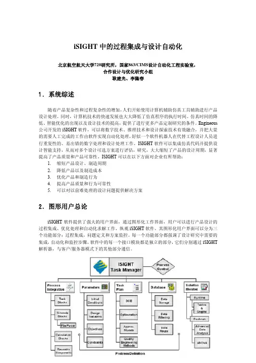
达索系统SIMULIA平台多参多学科优化软件Isight国内CAE仿真经过近二十年的发展，企业目前已不仅仅关注仿真本身，而是更多的考虑以下的三大领域：(1) 关注点从一般仿真分析向优化分析的过渡；(2) CAE仿真分析专业化，规范化和流程化；(3) CAE仿真分析问题的复杂化，涉及跨领域多学科复合问题。

我们将对上述三点分别进行解说。

1.1 从仿真分析到优化的过渡对于现今机械行业的从业人员来说，计算机辅助仿真分析方法已经被大家熟知并被广泛应用于各行各业，以实现仿真数字样机虚拟试验替代物理样机真实试验的最终目标。

随着国内CAE仿真分析水平的提升，在仿真分析方法和模式已经比较成熟的基础上，为了更有效的应用仿真分析结果，达到仿真分析结果指导产品设计的目的，优化方法和相应优化软件逐渐被引入到CAE部门的工作环节中。

如何应用优化软件搭建优化流程，以及通过什么样的优化方法和模式实现优化过程，成为很多企业CAE团队关注的问题。

根据上述需求，达索系统提供了Isight软件，作为多参数多学科优化工具平台，可以结合仿真分析工具（例如ABAQUS）实现仿真优化流程的搭建，解决产品设计与仿真联合优化的问题。

1.2 仿真规范化和流程化随着企业CAE团队的日益壮大与成熟，以及仿真数据的积累，这些企业都对仿真规范流程的搭建提出了迫切需求。

如今高性能计算资源极大丰富，并且可预见到在不久的将来量子计算机的发展和实用化将会带来计算资源的飞跃式增长。

对于CAE行业来说，计算机硬件将不再是仿真分析的瓶颈与桎梏，而大量的仿真模型处理任务和大量的待处理仿真数据将成为CAE团队的极大负担。

首先，如何将仿真流程规范化；其次，如何结合软件工具将相应流程固化；最终，如何尽可能使仿真流程自动化。

以上三点已经成为CAE行业想要发展壮大必须解决的问题。

在Isight中，我们可以通过有机的组合应用流程组件和应用组件创建仿真流程模板，通过源生应用组件和二次开发实现与第三方软件之间的调用和信息交互，通过Isight丰富的开发接口创建和开发仿真模板和定制模块。

1
根据图形界面结构图，现在论述各个功能模块的主要作用
2．1 任务管理
在 iSIGHT 中，任务管理是唯一可以方位软件所有模块的入口。任务管理负责控制设计 学习的执行。用户通过任务管理可以引导、管理任务的执行过程。在任务管理模块，克斯使 用的控制手段包括： 开始、停止、暂停、继续任务执行 选择运行模式－包括简单执行，任务计划和单一设计学习 多机器分布式任务 实行并行处理 检测点基础上的重新运行 单步调试
4
基础，为下述构建块的使用奠定了基础。 “构建块”的使用：在 iSIGHT 里，在系统里使用了“构建块”方法来定义模型的执行。 每一个构造块表示过程中的一个步骤。在 iSIGHT 中的基本构造块包括：任务块，计算块， 仿真块和定制块（自定义的用于支持商业化软件，如电子表格和 MSC/NASTRAN 模型的定 制块） 。其中各主要构造块的说明如下： 任务块：任务可以包含子任务或者 iSIGHT 中其他类型构造块。通过任务可以实现 层次化过程的表达，任务大大增强了在建立集成过程和设计执行策略时的柔性。 条件块：设计过程除了简单的顺序执行，还有其他的执行方式，通过条件块“If” ， “Case”和“While” ，可以方便用户建立过程控制逻辑。 计算块：计算块允许用户执行一些中间计算，例如单位转换，创建辅助参数或者执 行工具命令语言（Tcl）等。 仿真代码块：任意仿真代码可以通过 iSIGHT 的仿真代码块连接到系统中使用。用 户通过仿真代码块可以定义执行协议， 执行协议使描述设计问题求解中， 需要输入 什么文件，输出什么文件，执行程序的位置以及如何执行的执行手段综合。 电子表格 Excel 块： iSIGHT 为了方便实际使用电子表格的用户， 直接提供了与 Excel 的接口。这可以通过 iSIGHT 的 Visual Basic 插件直接创建 Excel 仿真代码块。 重用组件： 通过重用组件可以更加简化过程集成。 在设计过程中创建一个构造块以 后，可以把它保存到重用库里，这样就可以在不同组之间共享，或者作为模板来生 成相似过程块。极大的方便了过程的建立。 并行处理技术： 系统分析过程有时因为执行仿真代码会产生昂贵的费用。 在整个设计过 程里，因为所需系统分析的数量往往导致成倍成辈增加。但是在大多系统里，仿真代码可以 彼此独立运行，在许多设计分析技术里，多数设计点可以不同进行分析。因此在计算资源可 用的前提下，通过控制仿真代码和设计点的同步执行计算能力可以显著节省工程时间。 ISIGHT 软件提供了两种类型的并行执行方式：并行任务和并行设计技术的执行。 并行任务：在一个层次性的多任务定义里，存在一些任务，它们彼此之间不直接交 换数据。在这种情形下，称其为独立任务。整体问题中的独立任务就可以通过并行 执行来减少整个执行过程的时间。 设计技术并行执行： iSIGHT 的许多设计探索工具需要运行内在彼此独立的数据点。 这种情况下通过同时提供这些执行点的能力来实施并行技术处理。 松耦合、紧耦合相辅相成：在 iSIGHT 中，在 IPC 通信协议基础上，采用了松耦合和紧 密耦合结合的控制方式， 松耦合主要体现在对应用软件的仿真程序的执行方面； 紧密耦合表 现在可以集成基于 CORBA 的仿真代码进行设计过程的控制和优化。

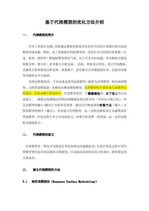
基于代理模型的优化方法介绍一，代理模型的简介许多工程设计问题，需要通过模拟实验来评估采用不同设计参数时的目标函数和约束函数。

例如，为了找到最佳的机翼形状，常常针对不同的形状参数（长度，曲率，材料等）模拟机翼周围的气流。

对于许多实际问题，单次模拟可能需要数分钟、数小时、甚至数天才能完成。

因此，类似设计优化、设计空间搜索、灵敏性分析和假设分析这种，需要数千、甚至数百万次模拟的任务，直接对原模型求解将是不可能的。

改善这种情况的一个办法就是使用近似模型（被称为代理模型，响应曲面模型，元模型或模拟器）来模拟高精度模拟模型。

代理模型的计算结果与原模型非常接近，但是求解计算量较小。

代理模型采用一个数据驱动的、自下而上的办法来建立。

一般假定原模拟过程的内部精确处理过程未知（有时也可能已知），但是该模型的输入-输出行为则非常重要。

通过在仔细选择的有限个点（输入）计算原模型的响应（输出），从而建立代理模型。

这一过程也被称为行为建模或者黑箱模型，但是这两个名字会造成歧义。

如果只涉及唯一的变量，这一过程也被称为曲线拟合。

二，代理模型的意义代理模型是一种包含试验设计和近似算法的建模技术，在设计优化过程中用代理模型替代原有的高精度分析模型，可以提高仿真优化的寻优效率，降低算法的计算成本。

三，建立代理模型的方法3.1 响应面模型法（Response Surface Methodology）响应面分析法是利用合理的试验设计方法并通过实验得到一定数据，采用多元二次回归方程来拟合因素与响应值之间的函数关系，通过对回归方程的分析来寻求最优工艺参数，解决多变量问题的一种统计方法。

计算原理：由于响应面法描述的是一组独立输入变量与系统输出响应之间某种近似关系，因此通常可用下式来描述输入变量和输出响应之间的关系。

()()εyy~x+=x式中，－响应实际值，是未知函数；－响应近似值，是一个已知的多项式；－近似值与实际值之间的随机误差，通常服从的标准正态分布。

基于isight的塔架门框结构的优化设计引言：伴随着社会经济的发展，建筑行业和建筑材料行业也在不断发展壮大。

传统的塔架门框结构的设计和制造已不能满足现代建筑的需求。

iSight是一款先进的塔架门框结构设计软件，它可以通过计算机模拟、分析和优化传统塔架门框结构。

在此基础上，本文以《基于iSight的塔架门框结构的优化设计》为主题，来探讨使用iSight 软件对塔架门框结构进行优化设计的方法，以期改善建筑材料的制造效率和节能等。

一、iSight介绍iSight是由美国麦迪逊数字图形有限公司开发的一款高级后处理软件，主要用于塔架门框结构的设计、分析和优化。

它具有以下优点：首先，对结构的变形、屈曲、弯曲、刚度和可靠性进行分析，使其能够根据使用情况选择最佳材料；其次，它可以进行实时优化，以期改善建筑材料的制造效率和节能率；另外，它还可以进行结构的几何校核，使设计和制造的工作更加准确和便捷。

二、iSight优化设计技术1、材料选择及参数优化：在执行iSight优化设计时，首先要选择合适的材料，以确定其参数，如弹性模量、材料厚度和其他属性。

接下来，进行参数优化，以便可以根据建筑需求和使用情况选择出最佳材料，并可以进行结构分析，以检查是否符合要求。

2、实时优化：iSight优化设计中的实时优化技术可以根据建筑需求和使用情况，模拟结构变形、屈曲、弯曲、刚度和可靠性，以改善建筑材料的制造效率和节能等。

实时优化的关键是，能够快速、准确地检测出一座建筑结构中的每一处缺陷，并尽可能地改善这些缺陷，以提高整体结构的可靠性和可承载性。

三、iSight的应用iSight可以用于几乎所有的建筑物的塔架门框结构的设计，其中包括大型建筑物和小型建筑物，如住宅、学校、桥梁、隧道、车站等。

使用iSight技术可以改善建筑材料的制造效率和节能率，降低建筑物的维护成本，并减少采购建筑材料的成本。

此外，iSight的设计技术还可以大大减少施工运行中发生的问题，减少不必要的施工损失。

14
专家系统技术（Expert System ）
启发式搜索（Directed Heuristic Search） 对整个设计空间使用专家知识 需要输入输出关系的知识 Engineous 拥有所有权的软件, 获得专利权
15
定制一种技术
调整参数（Tuning parameters） 简单的（Simple）
iSIGHT 基本培训
优 化
优化特征（ Optimization Features ）
任务计划（Task Plan）—技术组合
定制计划（ Customized Plan ） 预定义计划（ Predefined Plans ）
计划策略（ Plan Strategies ） 自动化技术选项 顾问/向导（Advisor/Guide）工具 – 问题空
使用时能够得到
5
标准的系统计划
优先计划（ Priority Ranked Plan ） 缺省，如果没有其它选择 基于知识的计划（ Knowledge Based Plan ） 局部计划（Exploitive） 全局计划（Explorative） 罚函数方向（ Penalty Direct ） 如果开始知道不可行区域
件
12
直接罚函数法（Direct Penalty ）
Hooke-Jeeves 外部罚函数（Exterior Penalty ） 罚函数法经常用于可行性设计仍没有确定时 罚函数法给目标函数增加了一个惩罚条件，
使之由约束问题转化为无约束问题
13
全局技术（Exploratory ）
遗传算法（Genetic Algorithm） 模仿自然选择的过程 选择种群大小和代次 模拟退火（Simulated Annealing） 模拟金属冷却期间的退火过程

优化算法分类范文优化算法是指经过改进或简化后的算法，可以提高计算机程序的性能和效率。

优化算法可以分为多种类型，下面将介绍最常见的几种。

1.贪婪算法：贪婪算法是一种利用贪心策略进行决策的算法。

它通过每次都选择局部最优解来实现全局最优解。

贪婪算法的特点是简单，易于实现，但不能保证获得全局最优解。

贪婪算法常用于求解最优路径、背包问题等。

2.分治算法：分治算法是一种将一个复杂问题拆分成多个子问题进行解决的算法。

每个子问题都是相互独立的，可以独立并行求解，最后通过合并子问题的解来得到原问题的解。

分治算法的典型应用有归并排序、快速排序等。

3.动态规划算法：动态规划算法是一种通过将问题划分为多个子问题，并存储子问题的解来避免重复计算的算法。

动态规划算法通常采用自底向上的方式进行计算，先计算出最小的子问题的解，然后根据已计算出的子问题解推导出更大规模的问题解。

动态规划算法适用于具有重叠子问题和最优子结构性质的问题，如背包问题、最短路径问题等。

4.回溯算法：回溯算法是一种通过穷举所有可能解来求解问题的算法。

在回溯过程中，不断地选择一个可能的解，然后进行下一步的探索，如果发现该解不能达到目标，就回退到上一步重新选择。

回溯算法适用于求解组合问题、排列问题、图的遍历等。

5.遗传算法：遗传算法是一种模仿自然界生物进化过程的优化算法。

它通过模拟基因的选择、交叉和变异来产生新的个体，然后根据适应度评估函数来选择优秀个体，再进行交叉和变异，不断迭代直到找到最优解。

遗传算法常用于求解问题、优化问题和机器学习问题。

6.模拟退火算法：模拟退火算法是一种模拟物质退火过程的全局优化算法。

它通过模拟退火的过程，逐渐放松约束条件，以接受更差的解并避免陷入局部最优解，最终找到全局最优解。

模拟退火算法常用于解决 traveling salesman problem、图着色问题等。

优化算法的目标是提高程序的性能和效率，因此在选择优化算法时，需要根据问题的性质、规模、约束条件等因素综合考虑。

� University of Southampton
� US Navy
� University of Tokyo
� University of Toronto

� Virginia Polytechnic Institute
13
国内客户对Isight的认可
� 自2003年正式成立进入中国市场以来，Isight迅速获得了国内航空、航天、 船舶、汽车、电子、兵器、高校等领先的研究部门认可，诸如： � 航天三院三部、一院12所、二院207所、航天802所、航空608所等； � 兵器201所、船舶701、船舶702所、核一院、电子14所等； � 一汽、长安、哈尔滨汽轮机厂、玉柴机器等； � 清华大学、北京航空航天大学、西北工业大学、北京理工大学等。
� U.S. Army TACOMARDEC
� Nippon Institute of Technology � Northwestern University � Tokyo Institute of Technology � Tsinghua University � University College of London � University of Aachen � University of Florida � University of Illinois
Isight 欧美市场占有率超过56%
日韩市场占有率超过70%
Isight4.5
中国市场占有率超过80%
GGEE公公司司超超过过 1100 年年 $$11220000万万开开 发发、、孵孵化化和和推推
广广
EEnnggiinneeoouuss 公公司司成成立立，，唐唐 兆兆成成博博士士为为创创 始始人人和和主主席席

优化算法分类范文概念：在计算机科学和运筹学中，优化算法又称为优化方法、算法或方法，是用于计算问题中最优解的算法。

它们根据定义的目标函数和约束条件，通过和迭代的过程来寻找问题的最优解。

1.经典算法分类：1.1穷举法：穷举法是一种简单直观的优化算法，通过遍历所有可能的解空间，然后找到满足条件的最优解。

缺点是计算复杂性高，当问题规模大时，计算时间会变得非常长。

1.2贪心算法：贪心算法是一种每一步都选择当下最优解的算法。

它通过局部最优解的选择来达到全局最优解。

但是贪心算法不能保证总是找到全局最优解，因为局部最优解并不一定能够达到全局最优解。

1.3动态规划：动态规划是一种将问题拆分成子问题并分解求解的方法。

它通过存储子问题的解来避免重复计算，从而提高计算效率。

动态规划通常用于求解具有重叠子问题结构的问题。

2.进化算法分类：2.1遗传算法：遗传算法是一种模拟自然进化过程的优化算法。

它通过使用选择、交叉、变异等操作，利用种群的进化过程来寻找最优解。

遗传算法适用于解决优化问题的空间较大或连续优化问题。

2.2粒子群优化算法：粒子群优化算法是一种模拟鸟群觅食行为的优化算法。

它通过模拟粒子在空间中的移动过程来寻找最优解。

粒子群优化算法适用于解决连续优化问题。

2.3蚁群算法：蚁群算法是一种模拟蚂蚁觅食行为的优化算法。

它通过模拟蚂蚁在空间中的移动过程来寻找最优解。

蚁群算法适用于解决离散优化问题和组合优化问题。

3.局部算法分类：3.1爬山法：爬山法是一种局部算法，它通过在当前解的邻域中选择最优解来不断迭代地改进解。

但是爬山法容易陷入局部最优解，无法找到全局最优解。

3.2模拟退火算法：模拟退火算法是一种模拟金属退火过程的优化算法。

它通过在解空间中随机选择解，并根据一定的退火策略逐渐降低温度来寻找最优解。

3.3遗传局部算法：遗传局部算法是遗传算法和局部算法的结合。

它首先使用遗传算法生成一组解，并使用局部算法对这些解进行改进和优化。

优化算法分类范文优化算法是解决实际问题的重要手段，它通过改进现有算法或设计全新算法的方式来提高问题的求解效率和质量。

优化算法按照不同的优化目标、技术思路和应用领域可划分为多个分类。

一、按照优化目标分类1.最优化算法：最优化算法着重于在给定的约束条件下，寻找最优解，常用于求解数学规划问题。

其中，凸优化算法和非凸优化算法是常见的两种类型。

-凸优化算法：凸优化算法可用于求解凸优化问题，通过寻找一个唯一的最小化或最大化值来满足约束条件。

常用的凸优化算法有梯度下降法、牛顿法、共轭梯度法等。

-非凸优化算法：非凸优化算法可用于求解非凸优化问题，其中目标函数或约束函数包含非凸部分。

常见的非凸优化算法有遗传算法、模拟退火算法、粒子群算法等。

2.多目标优化算法：多目标优化算法着重于同时优化多个目标函数，常用于多目标决策问题的求解。

其中，多目标进化算法是常用的一类多目标优化算法，包括支配排序遗传算法、多目标粒子群算法等。

3.非线性优化算法：非线性优化算法用于求解非线性优化问题，其中目标函数或约束条件包含非线性部分。

常见的非线性优化算法有拟牛顿法、信赖域方法、束方法等。

二、按照技术思路分类1.迭代优化算法：迭代优化算法通过迭代的方式逐渐接近最优解，常用于求解非线性优化问题。

其中，梯度下降法和牛顿法是常见的迭代优化算法。

2.随机优化算法：随机优化算法通过引入随机性来提高效率，并且可以避免陷入局部最优解。

常见的随机优化算法有遗传算法、模拟退火算法、粒子群算法等。

3.集成优化算法：集成优化算法通过将多个优化算法进行组合来提高算法的整体性能。

常见的集成优化算法有蚁群算法、遗传算法等。

三、按照应用领域分类1.智能优化算法：智能优化算法用于求解复杂问题和优化全局的非线性问题，典型的智能优化算法包括粒子群算法、遗传算法、蚁群算法、人工免疫算法等。

2.图像处理优化算法：图像处理优化算法用于改善图像质量、加速图像处理过程等，常见的图像处理优化算法包括模糊优化、降噪算法、去马赛克等。

优化算法分类范文优化算法是一种通过改进算法的设计和实现来提高计算机程序性能的方法。

它可以在不改变程序功能的前提下，减少计算时间、空间或其他资源的消耗。

优化算法可以应用于各种计算任务，例如图像处理、数据挖掘、机器学习和网络优化等领域。

优化算法可以分为多个分类。

下面将介绍一些常见的优化算法分类。

1.算法：算法通过在问题的解空间中最优解。

其中，穷举算法是最简单的一种方法，它通过枚举所有可能的解来找到最优解。

其他常见的算法包括贪婪算法、回溯算法、遗传算法和模拟退火算法等。

2.动态规划算法：动态规划算法通过将问题分解为子问题，并以一种递归的方式求解子问题，最终得到问题的最优解。

动态规划算法通常用于解决具有重叠子问题和最优子结构特性的问题。

3.近似算法：近似算法通过在有限时间内找到问题的近似最优解来解决NP难问题。

近似算法通常以牺牲精确性为代价，以获得计算效率。

常见的近似算法包括近似比例算法、贪婪算法和局部算法等。

4.随机算法：随机算法是一种基于随机性质的优化算法。

它通过引入随机性来避免算法陷入局部最优解，从而更有可能找到全局最优解。

随机算法包括蒙特卡洛方法、遗传算法和模拟退火算法等。

5.并行算法：并行算法是一种利用多个处理单元同时执行任务的算法。

它可以通过将问题划分为多个子问题，并在多个处理单元上同时求解来提高计算效率。

并行算法可应用于多核处理器、分布式系统和图形处理器等平台上。

6.启发式算法：启发式算法是一种基于经验和直觉的优化算法。

它通过利用问题的特定知识和启发式规则来指导过程，从而加速求解过程。

启发式算法包括人工神经网络、模糊逻辑和遗传算法等。

7.混合算法：混合算法是一种将多种优化算法结合起来使用的方法。

它可以通过利用各种算法的优势来克服单一算法的缺点，从而得到更好的性能。

混合算法通常通过分阶段或交替地使用不同的算法来求解问题。

总之，优化算法是一种通过改进算法设计和实现来提高计算机程序性能的方法。

不同的优化算法可以应用于不同类型的问题，并且可以根据问题的特点选择合适的算法。

4.1 iSIGHT优化基本问题4.1.1 iSIGHT集成软件的条件从一般意义上来说，只要是可执行文件（*.exe、*.bat）iSIGHT都可以进行驱动。

但是为了实现优化过程的自动化，要求所集成的数值分析软件能进行后台求解计算，且要有明确包含优化变量的输入、输出文件。

4.1.2 常用的输入文件的类型就目前市面上的数值分析软件而言，有以下两类文件可以作为输入文件：模型信息文件如上所述，数值分析软件一般分为三个模块，在数值建模结束后前处理程序便生成一个模型信息文件做为求解模块的输入文件，该模型文件包含了数值模型的各种信息，因此在优化的时候该文件便可以当作输入文件。

如，MSC.MARC的*.dat文件，LS—DYNA的的*.K文件等。

命令流或过程记录文件为了实现参数话建模与分析，好多数值分析软件中在提供菜单操作的同时也提供了相应地命令操作，并且可以把命令编程文件进行读入建模和分析，该文件常称为命令流文件。

另外，一些软件可以自动记录用户的每一步操作，并能输出相应地命令流文件，软件也可以读入该文件实现建模和分析，该命令流文件习惯称之为过程记录文件。

在使用模型信息文件当作输入文件的优化过程中，优化中在每次迭代过程中没有了建立模型的环节，因此其效率相对较高！而在用命令流或过程记录文件当作输入文件的优化中，在每次迭代分析时都从建模开始，故其计算所需要的时间相对较长。

然而，正是由于其每次迭代分析时都是从头开始建模分析，所以在相关变量的优化设计中，由于对模型信息文件的修改往往不能正确地反映模型的变化，故这时候就需要过程记录文件做为输入文件。

4.2 iSIGHT集成优化的一般步骤在工程上利用iSIGHT进行集成优化一般包括前期工作准备、过程集成、变量与算法设置以及过程监控与结果分析等步骤。

4.2.1 前期准备工作在集成优化之前的准备工作主要包括数值分析软件选择、初始计算以及熟悉相关文件等。

根据优化问题所要求的分析与求解任务，选择合适的数值分析软件进行优化设计计算。

isight优化基本问题4.1 iSIGHT优化基本问题4.1.1 iSIGHT集成软件的条件从⼀般意义上来说，只要是可执⾏⽂件（*.exe、*.bat）iSIGHT都可以进⾏驱动。

但是为了实现优化过程的⾃动化，要求所集成的数值分析软件能进⾏后台求解计算，且要有明确包含优化变量的输⼊、输出⽂件。

4.1.2 常⽤的输⼊⽂件的类型就⽬前市⾯上的数值分析软件⽽⾔，有以下两类⽂件可以作为输⼊⽂件：模型信息⽂件如上所述，数值分析软件⼀般分为三个模块，在数值建模结束后前处理程序便⽣成⼀个模型信息⽂件做为求解模块的输⼊⽂件，该模型⽂件包含了数值模型的各种信息，因此在优化的时候该⽂件便可以当作输⼊⽂件。

如，MSC.MARC的*.dat⽂件，LS—DYNA的的*.K⽂件等。

命令流或过程记录⽂件为了实现参数话建模与分析，好多数值分析软件中在提供菜单操作的同时也提供了相应地命令操作，并且可以把命令编程⽂件进⾏读⼊建模和分析，该⽂件常称为命令流⽂件。

另外，⼀些软件可以⾃动记录⽤户的每⼀步操作，并能输出相应地命令流⽂件，软件也可以读⼊该⽂件实现建模和分析，该命令流⽂件习惯称之为过程记录⽂件。

在使⽤模型信息⽂件当作输⼊⽂件的优化过程中，优化中在每次迭代过程中没有了建⽴模型的环节，因此其效率相对较⾼！⽽在⽤命令流或过程记录⽂件当作输⼊⽂件的优化中，在每次迭代分析时都从建模开始，故其计算所需要的时间相对较长。

然⽽，正是由于其每次迭代分析时都是从头开始建模分析，所以在相关变量的优化设计中，由于对模型信息⽂件的修改往往不能正确地反映模型的变化，故这时候就需要过程记录⽂件做为输⼊⽂件。

4.2 iSIGHT集成优化的⼀般步骤在⼯程上利⽤iSIGHT进⾏集成优化⼀般包括前期⼯作准备、过程集成、变量与算法设置以及过程监控与结果分析等步骤。

4.2.1 前期准备⼯作在集成优化之前的准备⼯作主要包括数值分析软件选择、初始计算以及熟悉相关⽂件等。

1054Optimization TechniquesThis chapter provides information related to iSIGHT’s optimization techniques. Theinformation is divided into the following sections:“Introduction,” on page106 introduces iSIGHT’s optimization techniques.“Internal Formulation,” on page107 shows how iSIGHT approaches optimization.“Selecting an Optimization Technique,” on page112 lists all availableoptimization techniques in iSIGHT, divides them into subcategories, and definesthem.“Optimization Strategies,” on page121 outlines strategies that can be used to select optimization plans.“Optimization Tuning Parameters,” on page124 lists the basic and advanced tuning parameters for each iSIGHT optimization technique.“Numerical Optimization Techniques,” on page147 provides an in-depth look at various methods of direct and penalty numerical optimization techniques.Technique advantages and disadvantages are also discussed.“Exploratory Techniques,” on page175 discusses Adaptive Simulated Annealing and Multi-Island Genetic Algorithm optimization techniques.“Expert System Techniques,” on page178 provides a detailed look at iSIGHT’s expert system technique, Directed Heuristic Search (DHS), and discusses how itallows the user to set defined directions.“Optimization Plan Advisor,” on page190 provides details on how theOptimization Plan Advisor selects an optimization technique for a problem.“Supplemental References,” on page195 provides a listing of additionalreferences.106Chapter 4 Optimization TechniquesIntroductionThis chapter describes in detail the optimization techniques that iSIGHT uses, and howthey can be combined to conform to various optimization strategies. After you havechosen the optimization techniques that will best suit your needs, proceed to theOptimization chapter of the iSIGHT User’s Guide. This book provides instructions oncreating or modifying optimization plans. If you are a new user, it is recommended thatyou understand the basics of optimization plans and techniques before working withthe advanced features. Also covered in the iSIGHT User’s Guide are the various waysto control your optimization plan (e.g., executing tasks, stopping one task, stopping alltasks).Approximation models can be utilized during the optimization process to decreaseprocessing cost by minimizing the number of exact analyses. Approximation modelsare defined using the Approximations dialog box, or by loading a description file withpredefined models. Approximation models do not have to be initialized if they are usedinside an optimization Step. The optimizer will check and initialize the models, ifnecessary. For additional information on using approximation with optimization, seeChapter8 “Approximation Techniques”, or refer to the iSIGHT User’s Guide.iSIGHT combines the best features of existing exploitive and exploratory optimizationtechniques to supplement your knowledge about a given design problem. Exploitationis a feature of numerical optimization. It is the immediate focusing of the optimizer ona local region of the parameter space. All runs of the simulation codes are concentratedin this region with the intent of moving to better design points in the immediatevicinity. Exploration avoids focusing on a local region, but evaluates designsthroughout the parameter space in search of the global optimum.Domain-independent optimization techniques typically fall under three classes:numerical optimization techniques, exploratory techniques, and expert systems. Thetechniques described in this chapter are divided into these three categories.This chapter also provides information about optimization techniques including theirpurpose, their internal operations, and advantages and disadvantages of the techniques.For instructions on selecting a technique using the iSIGHT graphical user interface,refer to the iSIGHT User’s Guide.Internal Formulation 107Internal FormulationDifferent optimization packages use different mathematical formulas to achieveresults. The formulas shown below demonstrate how iSIGHT approaches optimization. The following are the key aspects to this formulation:All problems are internally converted to a single, weighted minimization problem.More than one iSIGHT parameter can make up the objective. Each individual objective has a weight multiplier to support objective prioritization, and a scale factor for normalization. If the goal of an individual objective parameter is maximization, then the weight multiplier gets an internal negative sign.If your optimization technique is a penalty-based technique, then the minimizationproblem is the same as described above with a penalty term added.Objective :MinimizeSubject to :Equality Constraints:Inequality Constraints:Design Variables: for integer and realor iSIGHT Input Parameter member of set S for discrete parametersWhere :SF = scale factor with a default of 1.0W = weight a default of 1.0W i SF i ---------i ∑F i ×x ()h k x ()T et arg –()W k SF k---------0k 1=;=×…K ,W j SF j---------LB g j x ()–()×0≤W j SF j ---------g j x ()UB –()×0j 1…L ,,=;≤LB SF -------iSIGHTInputParameter SF ------------------------------------------------------------------------------UB SF-------≤≤108Chapter 4 Optimization TechniquesThe penalty term is as follows:base + multiplier * summation of (constraint violation ** violation exponent)The default values for these parametesr are: 10.0 for penalty base, 1000.0 forpenalty multiplier, and 2 for the violation exponent. These defaults can beoverridden with Tcl API procedures discussed in the iSIGHT MDOL ReferenceGuide.All equality constraints, h(x), have a bandwidth of+-DeltaForEqualityConstraintViolation. This bandwidth allows a specified rangewithin which the constraint is not considered violated. The default bandwidth is.00001, and applies to all equality constraints. You can override this default withthe API procedure api_SetDeltaForEqualityConstraintViolation.All inequality constraints, g(x), are considered to be nonlinear. This setting cannot be overridden. If an iSIGHT output parameter has a lower and upper bound, thissetting is converted into two inequality constraints of the preceding form. Similarto the objective, each constraint can have a weight factor and scale factor.iSIGHT design variables, x, can be of type real, integer, or discrete. If the type is real or integer, the value must lie within user-specified lower and upper bounds. Ifno lower and upper bound is specified, the default value of 1E15 is used. Thisdefault can be overridden though the Parameters dialog box, or through the MDOLdescription file.There is one default bound for each optimization plan, and a common global(default) bound value (1E15). During the execution of an optimization plan, theplan's bound value overrides the common value. When no optimization plan isused, the default common value is used.The significance of the default bound is that, from the optimization techniquespoint of view, iSIGHT treats each design variable as if it has both a lower andupper bound. If the type is discrete, iSIGHT expects that the value of the variablewill always be one of the values provided in the user-supplied constraint set.Internally, iSIGHT will have a lower bound of 0, and an upper bound of n-1, wheren is the number of allowed values. The set of values can be supplied through theinterface, or through the API procedures api_SetInputConstraintAllowedValuesand api_AddInputConstraintAllowedValues. The optimization technique controlsthe values of the design variables, and iSIGHT expects the technique to insure thatthey are never allowed to violate their bounds.Internal Formulation109 To demonstrate the use of iSIGHT’s internal formulation, some simple modifications to the beamSimple.desc file can be made.Note:This description file can be found in the following location, depending on your operating system:UNIX and Linux:$(ISIGHT_HOME)/examples/doc_examplesWindows NT/2000/XP:$(ISIGHT_HOME)/examples_NT/doc_examplesMore information on this example can be found in the iSIGHT MDOL Reference Guide.For illustrative purposes, there are two objectives in this problem:minimize Deflectionminimize MassThe calculations shown in the following sections were done using the following values as parameters:BeamHeight = 40.0FlangeWidth = 40.0WebThickness = 1.0FlangeThichness = 1.0After executing a single run from Task Manager, the corresponding output values can be obtained:Mass = 118.0Deflection = 0.14286Stress = 21.82929110Chapter 4 Optimization TechniquesObjective FunctionAll optimization problems in iSIGHT are internally converted to a single, weightedminimization problem. More than one iSIGHT parameter can make up the objective.Each objective has a weight multiplier to support objective prioritization, and a scalefactor for normalization. If the goal of an individual objective parameter ismaximization, then the weight multiplier gets and internal negative sign.Hence, the calculation of the objective function in this example is the following:(Mass)*(Objective Weight)/(Objective Scale Factor) + (Deflection)*(ObjectiveWeight)/(Objective Scale Factor)Substituting the values for this problem, we get:(118.0)*(0.0078)/(1.0) + (0.14286)*(169.49)/(1.0) = 25.13158Penalty FunctionThe Penalty Function value is always computed by iSIGHT for constraint violations.The calculation of the penalty term is as follows:base + multiplier * (constraint violation violation exponent)Constraint violations are computed in one the following manners:For the Upper Bound (UB): For the Lower Bound (LB): For the Equality Constraint:(Value - UB)(UB Constraint Weight)UB Constraint Scale Factor(Value - LB)(LB Constraint Weight)LB Constraint Scale Factor(Value - Target)(Equality Constraint Weight) Equality Constraint Scale FactorInternal Formulation 111In iSIGHT, the default values of the base, multiplier, and violation exponent are as follows:Base = 10.0Multiplier = 1.0Exponent = 2Constraint Scale Factor = 1.0 Constraint Weight = 1.0In the following example, you want to maximize a displacement output variable, but it must be less than 16.0. Suppose the current displacement calculated is 30.5. Also assume that you set our UB Constraint weight to 3.0, and the UB Constraint Scale Factor to 10.0. The equations would appear as follows:ObjectiveAndPenalty FunctionThe ObjectiveAndPenalty variable in iSIGHT is then just the sum of the Objective function value and the Penalty term. In this example, the ObjectiveAndPenalty variable would have the following value:25.13138 + 33990.645 = 34015.777It is the value of this variable that is used to set the value of the Feasibility variable in iSIGHT. Recall that the Feasibility variable in iSIGHT is what alerts you to feasible versus non-feasible runs. For more information on feasibility, see “iSIGHT Supplied Variables,” on page 101.Penalty = 10.0 + 1.0 * (30.5 - 16.0) * 3.010.02112Chapter 4 Optimization TechniquesSelecting an Optimization TechniqueThis section provides instructions that explain how to select an optimization plan. Akey part of this process is selecting an optimization technique. It provides an overviewof the techniques available in iSIGHT, and provides examples of which techniques youmay want to select based on certain types of design problems.Note:The following is intended to provide general information and guidelines.However, it is highly recommended that you experiment with several techniques, andcombinations of techniques, to find the best solution.Optimization Technique CategoriesThe optimization techniques in iSIGHT can be divided into three main categories:Numerical Optimization TechniquesExploratory TechniquesExpert System TechniquesThe techniques which fall under these three categories are outlined in the followingsections, and are defined in “Optimization Technique Descriptions,” on page114.Numerical Optimization TechniquesNumerical optimization techniques generally assume the parameter space is unimodal,convex, and continuous. The techniques including in iSIGHT are:ADS-based TechniquesExterior Penalty (page115)Modified Method of Feasible Directions (page116)Sequential Linear Programming (page117)Generalized Reduced Gradient - LSGRG2 (page115)Hooke-Jeeves Direct Search Method (page115)Selecting an Optimization Technique113 Method of Feasible Directions - CONMIN (page115)Mixed Integer Optimization - MOST (page116)Sequential Quadratic Programming - DONLP (page117)Sequential Quadratic Programming - NLPQL (page117)Successive Approximation Method (page117)The numerical optimization techniques can be further divided into the following two categories:direct methodspenalty methodsDirect methods deal with constraints directly during the numerical search process. Penalty methods add a penalty term to the objective function to convert a constrained problem to an unconstrained problem.Direct Methods Penalty MethodsGeneralized Reduced Gradient - LSGRG2Exterior PenaltyMethod of Feasible Directions - CONMIN Hooke-Jeeves Direct SearchMixed Integer Optimization - MOSTModified Method of Feasible Directions - ADSSequential Linear Programming - ADSSequential Quadratic Programming - DONLPSequential Quadratic Programming - NLPQLSuccessive Approximation MethodExploratory TechniquesExploratory techniques avoid focusing only on a local region. They generally evaluate designs throughout the parameter space in search of the global optimum. The techniques included in iSIGHT are:Adaptive Simulated Annealing (page114)Multi-Island Genetic Algorithm (page116)114Chapter 4 Optimization TechniquesExpert System TechniquesExpert system techniques follow user defined directions on what to change, how tochange it, and when to change it. The technique including in iSIGHT is DirectedHeuristic Search (DHS) (page114).Optimization Technique DescriptionsThe following sections contain brief descriptions of each technique available iniSIGHT.Adaptive Simulated AnnealingThe Adaptive Simulated Annealing (ASA) algorithm is very well suited for solvinghighly non-linear problems with short running analysis codes, when finding the globaloptimum is more important than a quick improvement of the design.This technique distinguishes between different local optima. It can be used to obtain asolution with a minimal cost, from a problem which potentially has a great number ofsolutions.Directed Heuristic SearchDHS focuses only on the parameters that directly affect the solution in the desiredmanner. It does this using information you provide in a Dependency Table. You canindividually describe each parameter and its characteristics in the Dependency Table.Describing each parameter gives DHS the ability to know how to move each parameterin a way that is consistent with its order of magnitude, and with its influence on thedesired output. With DHS, it is easy to review the logs to understand why certaindecisions were made.Selecting an Optimization Technique115 Exterior PenaltyThis technique is widely used for constrained optimization. It is usually reliable, and has a relatively good chance of finding true optimum, if local minimums exist. The Exterior Penalty method approaches the optimum from infeasible region, becoming feasible in the limit as the penalty parameter approaches ∞(γp→∞). Generalized Reduced Gradient - LSGRG2This technique uses generalized reduced gradient algorithm for solving constrained non-linear optimization problems. The algorithm uses a search direction such that any active constraints remain precisely active for some small move in that direction. Hooke-Jeeves Direct Search MethodThis technique begins with a starting guess and searches for a local minimum. It does not require the objective function to be continuous. Because the algorithm does not use derivatives, the function does not need to be differentiable. Also, this technique has a convergence parameter, rho, which lets you determine the number of function evaluations needed for the greatest probability of convergence.Method of Feasible Directions - CONMINThis technique is a direct numerical optimization technique that attempts to deal directly with the nonlinearity of the search space. It iteratively finds a search direction and performs a one dimensional search along this direction. Mathematically, this can be expressed as follows:Design i = Design i-1 + A * Search Direction iIn this equation, i is the iteration, and A is a constant determined during the one dimensional search.The emphasis is to reduce the objective while maintaining a feasible design. This technique rapidly obtains an optimum design and handles inequality constraints. The technique currently does not support equality constraints.116Chapter 4 Optimization TechniquesMixed Integer Optimization - MOSTThis technique first solves the given design problem as if it were a purely continuousproblem, using sequential quadratic programming to locate an initial peak. If all designvariables are real, optimization stops here. Otherwise, the technique will branch out tothe nearest points that satisfy the integer or discrete value limits of one non-realparameter, for each such parameter. Those limits are added as new constraints, and thetechnique re-optimizes, yielding a new set of peaks from which to branch. As theoptimization progresses, the technique focuses on the values of successive non-realparameters, until all limits are satisfied.Modified Method of Feasible DirectionsThis technique is a direct numerical optimization technique used to solve constrainedoptimization problems. It rapidly obtains an optimum design, handles inequality andequality constraints, and satisfies constraints with high precision at the optimum.Multi-Island Genetic AlgorithmIn the Multi-Island Genetic Algorithm, as with other genetic algorithms, each designpoint is perceived as an individual with a certain value of fitness, based on the value ofobjective function and constraint penalty. An individual with a better value of objectivefunction and penalty has a higher fitness value.The main feature of Multi-Island Genetic Algorithm that distinguishes it fromtraditional genetic algorithms is the fact that each population of individuals is dividedinto several sub-populations called “islands.” All traditional genetic operations areperformed separately on each sub-population. Some individuals are then selected fromeach island and migrated to different islands periodically. This operation is called“migration.” Two parameters control the migration process: migration interval, whichis the number of generations between each migration, and migration rate, which is thepercentage of individuals migrated from each island at the time of migration.Selecting an Optimization Technique117 Sequential Linear ProgrammingThis technique uses a sequence of linear sub-optimizations to solve constrained optimization problems. It is easily coded, and applicable to many practical engineering design problems.Sequential Quadratic Programming - DONLPThis technique uses a slightly modified version of the Pantoja-Mayne update for the Hessian of the Lagrangian, variable scaling, and an improved armijo-type stepsize algorithm. With this technique, bounds on the variables are treated in a projected gradient-like fashion.Sequential Quadratic Programming - NLPQLThis technique assumes that objective function and constraints are continuously differentiable. The idea is to generate a sequence of quadratic programming subproblems, obtained by a quadratic approximation of the Lagrangian function, and a linearization of the constraints. Second order information is updated by aquasi-Newton formula, and the method is stabilized by an additional line search. Successive Approximation MethodThis technique lets you specify a nonlinear problem as a linearized problem. It is a general program which uses a Simplex Algorithm in addition to sparse matrix methods for linearized problems. If one of the variables is declared an integer, the simplex algorithm is iterated with a branch and bound algorithm until the desired optimal solution is found. The Successive Approximation Method is based on the LP-SOLVE technique developed by M. Berkalaar and J.J. Dirks.Optimization Technique SelectionTable5-1 on page119, suggests some of the optimization techniques you may want to try based on certain characteristics of your design problem. Table5-2 on page120, suggests some of the optimization techniques you may want to try, based on certain characteristics of the optimization technique.118Chapter 4 Optimization TechniquesThe following abbreviations are used in the tables:Note : In the tables, similar techniques are represented by the same abbreviation/column. That is, the MMFD column represents the Modified Method of Feasible Directions techniques - ADS and the Method of Feasible Directions -CONMIN. The SQP column represents both DONLP and NLPQL versions of sequential quadratic programming.Optimization MethodsAbbreviation Modified Method of Feasible Directions - ADSMethod of Feasible Directions - CONMINMMFDSequential Linear Programming - ADSSLP Sequential Quadratic Programming - DONLPSequential Quadratic Programming - NLPQLSQP Hooke-Jeeves Direct Search MethodHJ Successive Approximation MethodSAM Directed Heuristic Search (DHS)DHS Multi-Island Genetic AlgorithmGA Mixed Integer Optimization - MOSTMOST Generalized Reduced Gradient - LSGRG2 LSGRG2Selecting an Optimization Technique 119* This is only true for NLPQL. DONLP does not handle user-supplied gradients.** Although the application may require some or all variables to be integer or discrete, the task process must be able to evaluate arbitrary real-valued design points.Table 5-1. Selecting Optimization Techniques Based on Problem Characteristics ProblemCharacteristicsPen Meth MMFD SLP SQP HJ SAM DHS GA Sim.Annl.MOST LSGRG2Only realvariablesx x x x x x x x x x**x Handles unmixedor mixedparameters oftypes real, integer,and discretex x x x x x Highly nonlinearoptimizationproblemx x x Disjointed designspaces (relativeminimum)x x x Large number ofdesign variables(over 20)x x x x x x Large number ofdesign constraints(over 1000)x x x x Long runningsimcodes/analysis(expensivefunctionevaluations)x x x x x Availability ofuser-suppliedgradients x x x x*x x120Chapter 4 Optimization TechniquesTable 5-2. Selecting Optimization Techniques Based on Technique CharacteristicsTechnique Characteristics MMFD SQP HJ SAM DHS GA SimulatedAnnealingMOST LSGRG2Does not requirethe objectivefunction to becontinuousx x x x xHandlesinequality andequalityconstraintsx*x x x x x x x xFormulationbased onKuhn-Tuckeroptimalityconditionsx x xSearches from aset of designsrather than asingle designx x**Used probabilisticrulesx xGets betteranswers at thebeginningxDoes not assumeparameterindependencex x x xDoes not need touse finitedifferencesx x x xOptimization Strategies121* This is only true for the Modified Method of Feasible Directions - ADS. The Method of Feasible Directions - CONMIN does not handle equality constraints.** First finds an initial peak from a single design, then searches a set of designs derived from that peak.Optimization StrategiesYou can specify a single optimization technique or a sequence of techniques, for a particular design optimization run. iSIGHT searches the design space by virtue of the behavior of the techniques, guided and bounded by any design variables and any constraints specified. Upon completion of an optimization run, you can switch techniques by either selecting another plan created with different techniques, or by modifying the current plan to apply a different optimization technique.Optimization plans with more than one technique can use strategies for combining the multiple optimization techniques. The following sections defines six optimization strategies.TechniqueCharacteristics MMFD SQP HJ SAM DHS GA Simulated Annealing MOST LSGRG2Not sensitive todesign variablevalues withdifferent orders ofmagnitudex x x Is easy tounderstandx Can be configuredso it searches in acontrolled, orderlyfashion xTable 5-2. Selecting Optimization Techniques Based on Technique Characteristics (cont.)122Chapter 4 Optimization TechniquesIn theory and in practice, a combination of techniques usually reflects an optimizationstrategy to perform one or more of the following objectives:“Coarse-to-Fine Search” on this page“Establish Feasibility, Then Search Feasible Region” on this page“Exploitation and Exploration,” on page123“Complementary Landscape Assumptions,” on page123“Procedural Formulation,” on page123“Rule-Driven,” on page124These multiple-technique optimization strategies are important to understand, and canserve as guidelines for those new to the iSIGHT optimization environment, or todesign engineers who are not optimization experts.Coarse-to-Fine SearchThe coarse-to-fine search strategy typically involves using the same optimizationtechnique more than once. For example, you may have defined a plan using theSequential Quadratic Programming technique twice, with the first instance calledSQP1 and the second instance called SQP2. The first instance, SQP1, may have a largefinite difference Step size, while the second instance, SQP2, may have a small finitedifference Step size.Advanced iSIGHT users may extend the coarse-to-fine search plan further bymodifying the number of design variables and constraints used in the search process,through the use of plan prologues and epilogues.Establish Feasibility, Then Search FeasibleRegionSome optimization techniques are most effective when started in the feasible region ofthe design space, while others are most effective when started in the infeasible region.If you are uncertain whether the initial design point is feasible or not, then anoptimization plan consisting of a penalty method, followed by a direct method,provides a general way to handle any problem.Optimization Strategies123 Advanced iSIGHT users can enhance the prologue at the optimization plan level so that the penalty technique is only invoked if the design is infeasible.Exploitation and ExplorationNumerical techniques are exploitive, and quickly climb to a local optimum. An optimization plan consisting of an exploitive technique followed by an explorative technique, such as a Multi-Island Genetic Algorithm or Adaptive Simulated Annealing, then followed up with another exploitive technique, serves a particular purpose. This strategy can quickly climb to a local optimum, explore for a promising region of the design space, then exploit.Advanced iSIGHT users can define a control section to allow the exploitive and explorative techniques to loop between each other.Complementary Landscape AssumptionsEach optimization technique makes assumptions about the underlying landscape in terms of continuity and modality. In general, numerical optimization assumes a continuous, unimodal design space. On the other hand, exploratory techniques work with mixed discrete and real parameters in a discontinuous space.If you are not sure of the underlying landscape, or if the landscape contains both discontinuities and integers, then you should develop a plan composed of optimization techniques from both categories.Procedural FormulationMany designers approach a design optimization problem by conducting a series of iterative, trial-and-error problem formulations to find a solution. Typically, the designer will vary a set of design variables and, depending on the outcome, change the problem formulation then run another optimization. This process is continued until a satisfactory answer is reached.If the series of formulations becomes somewhat repetitive and predictable, then the advanced iSIGHT user can automate this process by programming the formulation and。

isight nsga-ii案例以下是isight使用NSGA-II算法的一个案例：1. 初始化种群：随机生成一定数量的个体作为初始种群。

2. 非支配排序：利用Pareto最优解的概念将种群中的个体进行分级，非支配状态越高的个体层级越靠前。

首先找到种群中N(i)=0的个体，将其存入当前集合F1，然后对于当前集合F1中的每个个体j，考察它所支配的个体集 S(j)，将集合 S(j) 中的每个个体 k 的 n(k) 减去1，即支配个体 k 的解个体数减1（因为支配个体 k 的个体 j 已经存入当前集 F1），如 n(k)-1=0则将个体 k 存入另一个集F2。

最后，将F1 作为第一级非支配个体集合，并赋予该集合内个体一个相同的非支配序 i(rank)，然后继续对 H 作上述分级操作并赋予相应的非支配序，直到所有的个体都被分级。

重复步骤（a）-（b），直到所有个体处理完毕。

3. 拥挤距离：对于每个层级中的个体，计算其拥挤距离。

拥挤距离表示该解在目标空间中的分布情况，距离越小表示该解的分布越集中，即该解的竞争力越弱。

4. 选择操作：根据非支配排序和拥挤距离，从种群中选择一定数量的优秀个体进入下一代种群。

选择概率与非支配序和拥挤距离有关，非支配序越低、拥挤距离越大，被选择的概率越高。

5. 交叉和变异：对选中的个体进行交叉和变异操作，生成新的个体。

交叉操作可以采用单点交叉、多点交叉等方式，变异操作可以采用位反转、位翻转等方式。

6. 终止条件：重复步骤2-5，直到满足终止条件，如达到预设的最大迭代次数或种群中的最优解连续多次迭代没有明显提升等。

在以上过程中，NSGA-II算法可以在每一次迭代中找出种群中的Pareto最优解，并通过非支配排序和拥挤距离来指导算法搜索方向，从而使算法在多目标优化问题中表现出色。

同时，该算法不需要预设精英策略和共享参数等参数，可以自适应地处理不同规模和维度的多目标优化问题。