Virtual crack closure technique History, approach

第53卷第3期2021年6月Vol.53No.3Jun.2021南京航空航天大学学报Journal of Nanjing University of Aeronautics&Astronautics复合材料RTM十字形接头力学性能研究叶聪杰1，古兴瑾2，袁坚锋1，高苏旭2（1.上海飞机设计研究所，上海201210；2.南京航空航天大学航空学院，南京210016）摘要：针对某型飞机复合材料扰流板接头，选取典型十字连接区为研究对象，研究4点弯载荷作用下采用树脂传递模塑（Resin transfer moulding，RTM）成型工艺的十字接头典型件的极限承载能力，分析其损伤破坏模式，为复合材料RTM接头的设计强度分析提供参考。

论文通过典型细节件4点弯曲试验，测量了其极限承载能力，获得了试件典型破坏模式；同时基于商用ABAQUS有限元软件平台，建立了十字连接区典型细节件有限元模型，数值模拟了其损伤破坏过程。

通过比较数值模拟结果和试验结果，验证了数值模拟的可行性。

关键词：复合材料；树脂传递模塑；十字接头；数值模拟中图分类号：TB33文献标志码：A文章编号：1005⁃2615（2021）03⁃0381⁃07Mechanical Behavior of RTM Composite Cross JointsYE Congjie1，GU Xingjin2，YUAN Jianfeng1，GAO Suxu2（1.Shanghai Aircraft Design and Research Institute，Shanghai201210，China；2.College of Aerospace Engineering，Nanjing University of Aeronautics&Astronautics，Nanjing210016，China）Abstract:Aiming at the composite spoiler joint of a certain aircraft，the typical cross joint area is selected as the research object to study its ultimate load bearing capacity of the RTM（Resin transfer moulding）formed composite spoiler joint under the four point bending load.Its damage and failure mode is analyzed，and a reference for the design of RTM formed composite joints is provided.A finite element model of the typical detail of the cross connection area is established and its damage process is simulated using the commercial software ABAQUS.The simulated results agree well with the experimental data and thus the feasibility of the numerical simulations is verified.Key words:composite；resin transfer moulding（RTM）；cross joints；numerical simulation相对于金属材料，复合材料具有比较高的比强度、比刚度及良好的抗疲劳性和耐介质腐蚀性，因此在航空航天领域得到了广泛应用［1］。

Workshop 7Analysis of a DCB using VCCT (Abaqus/Standard)IntroductionIn this workshop we will consider crack growth in the double cantilever beam (DCB) specimen studied earlier using the virtual crack closure technique (VCCT). We will employ the same geometry, material properties as well as the mesh, boundary conditions and sets and surfaces defined in the cohesive surfaces model from the earlier workshop (see Figure W7–1 for geometry and load details).Figure W7–1 Schematic of the double cantilever beam specimen. PreliminariesIn this workshop, you will bond the two halves of the specimen and study crack growth resulting from the applied displacement. Previously, this problem was analyzed using both element-based and surface-based cohesive behavior. As part of this workshop, we will compare the results obtained from the VCCT model with those obtained using cohesive behavior.Open the model database file edited earlier (dcb-cohesive.cae). Begin by copying the model named coh-surfs to a model named vcct. If you did not complete the exercises with cohesive surfaces (Part 2 of the earlier workshop), follow the instructions given there to define the surfaces and sets, step, mesh, and contact properties and interaction before proceeding.The instructions that follow apply to the vcct model.W7.2Deleting obsolete features and defining the bond propertiesYou will begin by deleting features defined in the previous model that are not required in the VCCT model. Edit the contact interaction properties to delete the cohesive and damage properties inherited from the coh-surfs model. You will also define the bond properties at this stage.1.In the Model Tree, expand the Interactions Properties container and double-click the interaction property named coh.2.In the Edit Contact Property dialog box that appears, select Cohesive Behaviorfrom the list and click to delete it.3.In a similar fashion, delete Damage.4.In the editor, select Mechanical→Fracture Criterion and enter the data as shownin Figure W7–2:a.Select VCCT as the type.b.Select BK as the mixed mode behavior.c.Enter 0.1 as the tolerance.d.Enter 280 as the critical release rate for each mode and 2.284 asthe exponent.Figure W7–2 Bond properties.Editing contactAny contact formulation other than the finite sliding, surface-to-surface discretization can be used in conjunction with VCCT. As we used finite sliding for the cohesive surfaces model, we must change this to use small sliding.1.Expand the Interactions container in the Model Tree and double-click coh.2.In the Edit Interaction dialog box (see Figure W7–3) that appears, change thesliding formulation to Small sliding.3.In the Clearance tabbed page, select Uniform value across slave surface fromthe drop down menu next to Initial clearance. Enter 1e-7 in the data field, andclick OK.Note: The part instances are so positioned that there is no initial clearance between the bonded surfaces. After meshing, the nodes may have small initial overclosures that can cause several unnecessary severe discontinuity iterations. This is avoided by specifying a small initial clearance.Figure W7–3 Editing the predefined interaction for VCCT.Defining the bondYou will now define the bond.1.From the main menu bar, select Special→Crack→Create.2.In the Create Crack dialog box, select Debond using VCCT.3.In the Edit Crack dialog box:a.Select Step-1 as the initiation step.b.Select coh as the contact pair interaction.4.The editor appears as shown in Figure W7–4. Click OK to complete the operation.Figure W7–4 Bond definitionOutputEdit the default field output request to also include bond state BDSTAT and strain energy release rates ENRRT, found under the Failure/Fracture subsection (see Figure W7–4). These variables allow one to track the progression of damage at the interface through the course of a simulation, and are available for the slave surface.Figure W7–4 Editing the default field output requestJob1.In the Model Tree, double-click Jobs to create a job for this model. Name the jobdcb-vcct.2.Save your model database.3.Click mouse button 3 on the job name and select Submit from the menu thatappears. From the same menu, you may also select Monitor to monitor theprogress of the job and Results to automatically open the output database file for this job (dcb-vcct.odb) in the Visualization module.ResultsWhen the job is complete, open dcb-vcct.odb in the Visualization module.1.Plot the deformed shape and contour the stress distribution in the specimen.Animate the response (increasing the scale factor so that the deformation in theearly stages can be seen more clearly). Figure W7–8 shows the final specimenconfiguration and the Mises stress distribution at the end of the job.Figure W7–8 Mises stress distribution2.To locate the crack tip more precisely, contour the output variable BDSTAT (bondstate), which is a numerical estimate of the extent of damage at the interface. Itranges from 0 for slave nodes that are fully detached from the master surface to 1 for fully bonded slave nodes. Animating the response allows you to track crack-propagation. Figure W7–9 shows a contour plot of BDSTAT for a magnified view of the crack roughly half way through the simulation (t=0.5). One can also use the strain energy release rates (ENRRT) for the same purpose.Figure W7–9 Contour plot of bond state BDSTAT at time = 0.53.Create a force-displacement plot as described earlier.4.Save the curve as VCCT and plot it.5. A comparison of the force-displacement response obtained using VCCT with thatobtained using element-based and surface-based cohesive behavior is shown inFigure W7–10. The results are in excellent agreement.Figure W7–10 Comparison of force-displacement response between VCCT and element-based and surface-based cohesive methods.Note: A script that creates the complete model described in these instructions is available for your convenience. Run this script if you encounter difficulties following the instructions outlined here or if you wish to check your work. The script is namedws_composites_dcb_answer.pyand is available through the Abaqus fetch utility.。

COVER SHEETTitle: Simulation of Arbitrary Delamination Growth in Composite Structures Using the Virtual Crack Extension Method Authors: Brett R. DavisPaul A. WawrzynekAnthony R. IngraffeaABSTRACTA finite-element-based toolset has been developed to simulate arbitrary evolution of 3-D, geometrically explicit, interlaminar delaminations in composite structures. A new energy-based growth formulation uses the virtual crack extension (VCE) method to predict point-by-point growth along the delamination front. The VCE method offers an accurate and computationally efficient means to extract both energy release rate, , and rate of change of energy release rate, , from a single finite element analysis. A new VCE implementation is used to decouple and compute 3-D, mixed-mode, fracture parameters, permitting the use of mixed-mode growth criteria. The parameters create an influence matrix that relates an extension at one point to the energy release rate elsewhere along the delamination front. The use of the matrix, in conjunction with an iterative approach that continually updates the delamination configuration by re-meshing, enables the prediction of arbitrary delamination evolution. The numerical techniques and formulations implemented allow a delamination to grow by the rules of mechanics and physics, while reducing computational artifacts, e.g. mesh bias. The evolution of an initial embedded elliptical delamination under central point-loads into a circular configuration is simulated as a proof-of-concept for the new growth formulation.INTRODUCTIONLaminated, fiber-reinforced, composite materials are used in a variety of applications, including the aerospace and marine industries. Although laminated composite structures have been in use for decades, fully understanding and accurately predicting their failure mechanisms remains a significant challenge. The current work seeks to address this challenge for one of the most common modes of failure: delamination. A variety of finite-element-based approaches has been Cornell University, School of Civil and Environmental Engineering638 Frank H.T. Rhodes Hall, Ithaca, NY 14853, U.S.A.developed to handle the problem of progressive delamination growth. These include damage mechanics [1], cohesive crack models [2], nodal release methods via the virtual crack closure technique (VCCT) [3,4] and the extended finite element method (XFEM) [5]. This paper describes the development of a new approach, one that reduces computational limitations, freeing the mechanics and physics to dictate the evolution of the delamination.Perhaps the most widely utilized of the aforementioned are cohesive zone models and nodal release methods. However, these methods limit the characterization of delamination growth by constraining the evolution to the geometry of the predetermined finite element mesh. Cohesive zone elements use traction-displacement curves to govern behavior at the delamination front. When the traction-displacement relationship reaches its limit, i.e. maximum displacement, and zero traction, the cohesive element is eliminated, thus extending the delamination. Alternatively, fracture mechanics methods are used to calculate stress intensity factors or energy release rates at the front, and identify nodes to be released to extend the front. In either case, the delamination path will only follow existing element boundaries, restricting the direction and distance of the predicted advance of the front. These growth prediction approaches have the potential to produce saw-tooth, jagged delamination fronts that do not match physical configurations, as seen in Figure 1.To minimize these limitations, one can use a heavily refined mesh around the front, greatly inflating the computational cost, or one can produce meshes constructed with knowledge of the expected delamination growth pattern. However, this latter technique contradicts the notion of arbitrary evolution by linking a physical feature, delamination shape, with a computational artifact, the mesh. For example, with an initial circular flaw, one might design a mesh that contains an organization of elements in a concentric circular pattern around the initial delamination, Figure 2. However, of interest here is what happens when theFigure 1. Jagged saw-tooth delamination growth via the nodal release method - resulting inmesh biased constrained growth. From [3].initial delamination geometry is complex, and the growth pattern is unknown. Meshes should not provide a predetermined undue bias that obfuscates the physical results of a simulation.This work proposes a new, general approach for the simulation of geometrically explicit delamination evolution. The geometry of the delamination front is continually updated and the finite element model is appropriately re-meshed around the updated front. This procedure of updating the delamination configuration and then re-meshing ensures the arbitrary nature of the evolution. The advance of the delamination and creation of new surface area are governed by a new energy-based formulation.An incremental-iterative procedure utilizes the growth formulation to calculate point-wise advances along the delamination front. The geometry of the delamination drives the finite element simulation; the growth is not dictated by the finite element mesh, but by the mechanics and physics embedded within the energy-based growth formulation.To use effectively the new energy-based growth formulation, fracture mechanics parameters must be accurately and efficiently calculated. A novel contribution of the new energy-based growth formulation is the use of the first order derivative of the energy release rate with respect to the delamination length, the rate of energy release rate, . The parameter, in the 3-D sense, serves as an influence matrix that relates how an extension, , at one point affects the energy release rate, , elsewhere along the front. The virtual crack extension (VCE)Figure 2. Pre-designed finite element mesh that adheres to expectedgrowth pattern – resulting in mesh biased constrained growth.method has been determined to be the most appropriate fracture mechanics tool, since it can extract both energy release rates and rates of energy release rate with a single finite element analysis. Other means of calculating the parameter require a costly and time consuming finite difference approach. Another novelty presented is a VCE implementation that permits the decomposition of the energy fracture parameters, thus allowing the future use of mixed-mode fracture criteria.The simulation technique incorporates three main components: 1) explicitly representing delaminations with re-meshing capabilities, 2) fracture calculations using the VCE method, and 3) prediction of growth using the new energy-based formulation. It should be noted that the techniques developed are independent. The energy-based growth formulation can be implemented using the VCCT (which has been done by the authors), or even be applied within the XFEM environment. The simulation methodology developed aims to achieve arbitrary delamination growth through representing the delamination as a geometric feature while reducing finite element bias.The following sections will introduce the VCE method, providing background and a general framework. The implementation of the new 3-D, mixed-mode decoupling of energy release rates will be discussed. Verification results will be presented showing its effectiveness. The energy-based growth formulation will be introduced, describing the foundation and implementation of the method. Finally, the simulation of an embedded elliptical delamination subject to equal and opposite delamination face point loads is offered as a proof-of-concept for the new growth formulation.THE VIRTUAL CRACK EXTENSION METHODThe virtual crack extension (VCE) method, also known as the stiffness derivative method, is an energy approach first introduced by Dixon and Pook [6] and Watwood [7], and further developed by Hellen [8] and Parks [9]. Early VCE calculations utilized explicit perturbations of the finite element meshes to approximate the method’s required stiffness derivatives. Th e finite difference approach of calculating derivatives often introduces geometric approximation and numerical truncation errors. Haber and Koh [10] developed a variational approach that eliminated the need for perturbations for stiffness derivative calculations. Lin and Abel [11] derived a similar method, rooted in variational principle theory, but generalized and simplified the required integration of [10]. Additionally, and importantly to the energy-based growth formulation herein, the approach of [11] permits the derivation of expressions for higher order derivatives of energy release rates. Hwang utilized the formulation of [11], generalizing the direct-integration approach for 2-D [12], multiply cracked bodies [13], and planar 3-D cracks [14]. The salient features of the VCE method are the accurate calculation of energy release rates and their derivatives, with a single finite element analysis.Virtual Crack Extension FormulationThis section outlines the explicit expressions derived using the variational approach for the 3-D energy release rates and their derivatives. The followingformulation demonstrates the mathematical development of the VCE method. For a more complete mathematical derivation and discussion see [11] and [14].The potential energy, , of a finite element system is given by(1)where , , and are the nodal displacement vector, the global stiffness matrix and the applied nodal force vector, respectively.The energy release rate, , at front position is defined as the negative derivative of the potential energy with respect to an incremental front extension, , at that position.(2)For simplicity, it is assumed that nodal forces are not influenced by the incremental virtual extensions. Therefore, the variational force term, , goes to zero. The necessary parameters for a local energy release rate calculation at position require nodal displacements and the variation in stiffness due to an incremental crack extension. The simplification reduces equation (2) to:(3) It should be noted, however, if crack-face pressures, thermal, and/or body force loadings are considered, the variational force term must be included throughout the expressions and derivations.The expression for the first order derivative of the energy release rate follows from the previous equations, by taking the variation of in equation (3) with respect to another incremental crack extension, , at position .(4) The variation of displacements extends directly from the variation of the global finite element equilibrium equation, , with respect to an incremental crack extension, .(5)Rearranging equation (5) and applying the simplifying assumption of , yields the expression for the variation of nodal displacements:( )(6)The remaining derivations of the expressions for the stiffness derivatives can be found in [14]. These require a ‘strain-like’ matrix created by the virtual extensions applied to th e front elements. The ‘strains’ are created by geometry changes of the finite elements in parametric space. Through the Jacobian and basis functions, variations in the strain-displacement matrices can be formulated, providing the components necessary for the stiffness derivative integrals.Three-Dimensional Mixed-Mode Decomposition of Energy Release Rates Several methods have been proposed to decompose energy release rates using the VCE method. [15] attempted to draw concepts used from the decomposition of the -integral into and . However, inaccuracies were discovered in the term when mode-II was dominant. [10] proposed a general 2-D method using Betti’s reciprocal theorem and Yau’s mutual energy representation. [11] used a similar approach that marries actual displacement fields with analytic solutions for pure mode-I and pure mode-II behavior. This is comparable to methods used in the interaction -integral [16,17]. Ishikawa [18] developed a 2-D approach that first decomposed the displacements into mode-I and mode-II components using symmetry and skew-symmetry about the delamination front. The decomposed displacements were then used in standard VCE equations to calculate the mixed-mode energy release rates. This method was extended to 3-D by Nikishkov and Atluri [19] for the -integral, and identified by [14] as a feasible 3-D approach for mode decomposition within the VCE method. One limitation to the symmetric/skew-symmetric technique is that a symmetric mesh is required around the front. This limitation is overcome through use of a front template that will be discussed later in the implementation section.In the decomposition technique, displacement fields around a straight front can be separated into mode-I, II and III components. For an arbitrary front, the use of a local front coordinate system is required, Figure 3. A point-by-point coordinate transformation scheme is employed to essentially ‘straighten’ the front locally so the symmetric decomposition method can be used.Once the front is in a local orientation, the mode-I, mode-II, and mode-III deformations can be decomposed with respect to the delamination plane along the local axis. Taking advantage of the symmetry of the finite element meshFigure 3. Local delamination front coordinate system.surrounding the front, displacements at point ()and at (), are used to decompose mode-I, mode-II and mode-III displacements at .(7){}(8){}(9){}(10)With the displacements decomposed, and a transformed local stiffness derivative, denoted by the subscript , available, the following equation yields the mixed-mode energy release rates:, where (11) Virtual Crack Extension ImplementationThis section discusses the implementation of the VCE method, and the various numerical schemes employed to improve performance. The core of the VCE method has been implemented as a MATLAB post process. The MATLAB code reads in finite element information that identifies front nodes, elements, etc., and nodal displacements. The front is surrounded by a template comprising three rings of elements whose geometry can be carefully controlled. This satisfies the symmetric requirements of the mode decomposition method discussed previously and facilitates accurate fracture parameter calculations. The elements directly surrounding the front are either 20-noded brick or 15-noded wedge serendipity quarter-point elements,Figure 4.The VCE procedure is applied across the front elements. Non-zero contributions to the stiffness derivatives occur only over elements involved with the virtual extensions. These elements are isolated for stiffness derivative calculations that are summed appropriately for a given virtual extension. Certain considerations must be addressed when dealing with a 3-D delamination. Along a 3-D front, virtual extensions between adjacent positions have an interaction component that must be accounted for in second order stiffness derivative calculations (). Also, the 3-D virtual extensions have an area associated with them depending on the element size that must be used to normalize the energy release rates and their derivatives. Since the formulation utilizes the variational approach, the virtualextension applied can be of unit length; no optimized distance must be determined, thereby simplifying the implementation.To ease the effort of computations, the use of an intermediate global force derivative parameter is employed. For each element involved with a particular front node , first order stiffness derivatives are calculated then multiplied by the element nodal displacements.(12)The force derivative parameter is mapped into a global environment and summed over the elements for the current front position. The global force derivative for each front node is stored in a matrix. This matrix is of size: number of degrees of freedom by number of front nodes, and is utilized in the calculation of the variation in displacements. Significant computational cost lies in the execution of equation(6). Unlike the stiffness derivative, the variation in displacements is a global calculation. The virtual extensions have an influence on all points within the finite element model. Equation (6) requires -number of back solves with the symmetric global stiffness matrix and global force derivative. To accelerate the calculation and alleviate memory issues associated with the back solves, a standalone, parallelizable, sparse direct solver, MUMPS (MU ltifrontal M assively P arallel sparse direct S olver), is utilized.VCE calculations can be conducted at corner or midside nodes along the front. The selection of corner or midside nodes alters the profile of the virtual extension: the former is linear, the latter quadratic. It was determined through a previous numerical investigation that calculations at corner nodes outperformed midside nodes. This observation agrees with results published in the literature for other methods [20].Also incorporated in the implementation is the ability to carry out the numerical integration over one or two rings of elements, Figure 5. The single ring of integration comprises only quarter-point elements. The second ring utilizes the quarter-point elements and the next layer of surrounding brick elements. The theory behind adding the second ring is to improve results by effectivelyshifting Figure 4. 20-noded brick and 15-noded wedge quarter point elements used to surround thedelamination front.X2X1Figure 5. (a) 1-ring and (b) 2-ring elements involved in numerical integration for the VCE method.Top figures show the initial configuration. Bottom figures show the applied virtual extensions. the area of high virtual strain caused by the virtual extensions away from the singular elements, to elements where field gradients are not as severe. The singular elements around the delamination front experience negligible virtual strain, i.e. shape and volume change in the element, and the brunt is moved to the second ring, Figure 6. In the same numerical investigation alluded to earlier, the second ring of integration was shown to provide more accurate results for both energy release rates and rates of energy release rate.Herein, results will be reported only for the simplest, albeit still effective, form of the mixed-mode VCE method that uses quarter-point brick elements and a single ring of numerical integration at corner nodes along the front.Verification Results for 3-D, Mixed-Mode Virtual Crack Extension Method This section presents preliminary verification for the newly implemented 3-D, mixed-mode VCE method. To check the formulation and implementation, analytical displacements [22] from prescribed energy release rates were imposed on a straight front. Four scenarios were analyzed: 1) pure mode-I, 2) pure mode-II, 3) pure mode-III, and 4) mixed-mode I/II/III. In each instance an energy release rate of unity was prescribed.For brevity, the results from the mixed-mode I/II/III scenario are shown in Figure 7. The pure mode-I, II, and III situations yielded similar levels of accuracyfor their respective energy release rates. For each analysis, the decomposed energy release rates were within a fraction of one percent of the prescribed value. The energy release rates also agreed well with the total energy release rate calculations, verifying the known linear relationship.ENERGY-BASED PREDICTION OF DELAMINATION GROWTHThe new energy-based growth formulation and implementation draw inspiration from experiences in plasticity. Both plasticity and delamination growth are characterized by behavioral transitions. These are denoted by a critical limit, for plasticity, the yield stress, and for delamination growth, a critical energy release rate. With this general connection between delamination growth and plasticity, a new formulation is developed for discretized front evolution.Energy-Based Growth FormulationThe formulation extends directly from an expansion of the energy release rate.(13)The current energy release rate, , is expanded into three components: the previous energy release rate prior to the load increment , , a portion due to the change in loading, , and a portion due to extension, . HereFigure 6. 2-ring virtual extension showing area of high virtual strain along the delamination front.Figure 7. Mixed-mode energy release rate results using the 3-D VCE decomposition method.characterizes the change in energy release rate with respect to the loading, is the aforementioned influence matrix, and is the extension increment. The expanded energy release rate forms a general stability equation that can be manipulated to calculate growth increments for an arbitrary front for a given load change.A local front failure criterion must be selected. For simplicity, a local critical energy release rate, , is set as the failure criterion. However, the formulation is not limited to this form of criterion. Effective energy release rates comprised of decomposed modes subject to power laws, etc. can easily be used with the formulation.Two primary assumptions constrain the growth formulation to make results physically meaningful. The first asserts that the front cannot retreat, equation (14). The second restricts the current energy release rate from exceeding the critical criterion value, equation (15). Physically, the current front cannot exist at energy levels above the material’s critical value, thus indicating a necessary change – i.e. the shape of the front.(14)(15)Substituting the local failure criterion, , into the general stability equation (13), yields the general growth condition.(16)This stability equation can be incorporated into an incremental loading schemewhere resulting front extensions are calculated, determining a stable shape for each load increment.Energy-Based Growth ImplementationThe energy-based growth formulation is imbedded within an incremental-iterative procedure. This procedure requires an initially stable configuration. Thedelamination is then incrementally loaded. For each load increment, a growthcondition is checked. If growth is detected, an iterative approach is employed usingthe energy-based growth formulation to achieve a stable configuration for thatgiven load increment. If growth is not detected, the algorithm is allowed to proceedto the next load increment and continue on in the simulation. Figure 8 depicts theiterative scheme of the simulation technique that incorporates finite element modelgeneration, analysis, fracture mechanics calculations, and the growth formulation.As introduced previously, the mixed-mode virtual crack extension (VCE)method is used to calculate energy release rates along the front. Energy release rates need to be extracted for both the stable configuration, { }, and after the load increment, {}. Here {}denotes a vector of quantities, i.e. the energy release rate for each point along a discretized front.At each load level, the VCE results are compared to critical values to determineif a growth condition is reached. The initial load level should be stable, meaning for all points along the front { }{}. After the load increment is applied, the energy release rates are checked again. Positions along the front are separated into mobilized, {}{ }, and stationary points, {}{ }. As the notation implies, the mobilized points are those that are expected to advance, where the stationary points, remain at their current locations. The mobilized points exceed the critical criterion for the given load increment, which is not physically attainable, indicating that an update in the front geometry is required.The stability equation is rearranged and employed to determine the portion of the load increment, , that results in the mobilized positions going from stableFigure 8. Simulation flow chart outlining use of finite element analysis, the VCE method, and the energy-based growth formulation in an iterative scheme.{ } levels to the critical values, {}. To determine , it is assumed that the front geometry is unchanged, i.e. . Herein, the mobilized notation is dropped for clarity.{}{}{ }(17)The {} term is obtained through a finite difference calculation between {} and { }. The value for each of the mobilized positions along the front is subtracted from the total load increment, , to attain the portion of the load increment that contributes energy to the system resulting in extension.{ }{}{}(18) In the next stage of the calculation, it is assumed that operations are centered at the local failure criterion. This sets {}{}. The added energy { } term is inserted back into the reorganized stability equation to calculate the delamination extensions for the mobilized positions, {}.{}{}{}{ }[]{}(19){}{}(20){}[]{}{ }(21) The [] notation signifies a matrix. Equation (21), with the use of the [] influence matrix, makes this method unique and capable of capturing arbitrary delamination growth.Each mobilized position along the front is advanced according to {}in an outward normal direction. The front geometry is updated, and re-meshed. With an updated finite element model, the iterative process is continued. The updated front geometry is loaded at the initial stable level prior to . A new { }is calculated. The load increment is applied to the updated configuration. A new {}is calculated. A new set of mobilized and stationary nodes areidentified. The previously described procedure is repeated with the new mobilized nodes, calculating the next iteration of extensions. The iterations are continued until a stable configuration is reached for the given load increment. The stability of the front geometry is achieved when, for all positions along the front, the energy release rates are below the failure criterion.SIMULATION AND RESULTSTo test the formulation and implementation of the energy-based growth formulation, a proof-of-concept simulation was designed. The finite element re-meshing, front advances, and model generations were carried out by in-house software. The models generated were imported into the ABAQUS finite element software. ABAQUS served as both the finite element environment and solver. The virtual crack extension (VCE) method used the ABAQUS results to calculate the necessary fracture mechanics parameters. The energy-based growth formulation was then employed to calculate point-by-point extensions for a given load increment.An initial, embedded elliptical delamination, aspect ratio 2:1, in an isotropic material subjected to centrally applied point loads to the surfaces was simulated, Figure 9. Simple supports were used to prevent rigid body motion. For this example, a constant local critical energy release rate was chosen as the failure criterion. This configuration was selected because of its inherently stable growth. The elliptical geometry offers an opportunity to view non-uniform growth, rather than simulating a circular delamination that grows concentrically.The load was separated into 25 increments. A stable configuration was reached for each load increment. On average, each increment required four iterations. The initially elliptical delamination evolved along the minor axis, eventually bowing into a circular configuration. Figures 10-15 show a sample of the stable configurations for selected load increments.To assess the quantitative accuracy of the energy-based growth formulation, the simulation was continued to observe the circular growth pattern (Figures 14-15). Five concentric circular growth increments were simulated. An average percent difference of 0.1% was found for the simulated radii when compared to an analytical expression [21].Figure 9. Geometry and boundary conditions for proof-of-concept simulation.。

四Abaqus在复合材料领域的优势4.1 复合材料介绍4.1.1 复合材料的应用复合材料有许多特性：1、制造工艺简单2、比强度高，比刚度大3、具有灵活的可设计性4、耐腐蚀，对疲劳不敏感5、热稳定性能、高温性能好由于复合材料的上述优点，在航空航天、汽车、船舶等领域，都有广泛的应用。

复合材料的大量应用对分析技术提出新的挑战。

4.1.2 复合材料的结构复合材料是一种至少由两种材料混合而成的宏观材料，其中的一种材料被称作基体，其它的材料称作纤维。

其中纤维可以包含很多不同的形式：离散的宏观粒子，任意方向的短纤维，规则排列的纤维和织物。

1)单向纤维层合板----冲击分析2)编织复合材料---- 挤压分析3)蜂窝夹心复合材料----不可见冲击损伤分析基体和纤维的存在形式以及材料属性对于复合材料的力学行为有着很大的影响。

改变纤维和基体的属性目的就是在于生成一种复合材料具有如下性质：1）低成本：原型，大规模生产，零件合并，维修，技术成熟。

2）期望的重量：轻重量，比重分配合理。

3）改进的强度和刚度：高强度/高刚度比。

4）改进的表面属性：良好的耐腐蚀性，表面抛光性好。

5）期望的热属性：较低的热传导性，热膨胀系数较低。

6）独特的电属性：具有较高的绝缘强度，无磁性。

7）空间适应性：大部件，特殊的几何构型。

4.1.4 复合材料的有限元模拟根据不同的分析目的，可以采用不同的复合材料模拟技术：1）微观模拟：将纤维和基体都分别模拟为可变形连续体。

2）宏观模拟：将复合材料模拟为一个正交各向异性体或是完全各向异性体。

3）混合模拟：将复合材料模拟为一系列离散、可见的纤维层合板。

4）离散纤维模拟：采用离散单元或是其它模拟工具进行模拟。

5）子模型模拟：对于研究加强纤维周围点的应力集中问题比较有效。

微观模拟：纤维-基体的单胞模拟混合模拟：层合板的混合模拟Abaqus中复合材料的单元技术Abaqus中复合材料的单元技术主要为三种：分层壳单元、分层实体单元以及实体壳单元。

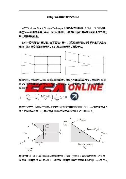
ABAQUS中疲劳扩展VCCT技术VCCT（Virtual Crack Closure Technique）指的是虚拟裂纹张合技术，这个技术是根据Irwin能量理论提出来的，其核心思想为：假设裂纹在扩展中释放的能量等于闭合裂纹所需要的能量。

我们来看裂缝的扩展过程，在下图的扩展中，我们假设裂缝的前缘形状是不发生变化的，即扩展后裂缝的张开尺寸和扩展前的张开尺寸是相等的。

如图所示，当裂缝从左图扩展到右图的时候，假设其能量释放率为G I，而裂缝扩展所需要的临界能量释放率为G IC，那么，当G I>G IC时，裂缝就会发生扩展，即裂缝的扩展准则为在这个公式中，b和d分别表示的是单元上裂尖位置的宽度和长度，F v,2,5指的是节点2和5之间的垂直力，v1,6表示节点1和6之间的垂直位移（如下图所示）。

我们注意到，这个理论能够预测裂缝的扩展，但是只适用于I型裂缝的状态，对于普通裂缝，则需要对理论进行修正，这时候，就需要用等效应变能量释放率G equiv来表示。

在通用状态下，我们用这个公式替代上面的扩展准则，因为G equiv是包含三种裂缝能量释放率的，我们来看看它的表达式：在ABAQUS中，对G equiv的计算有三种方法，包括BK法，power low方法和Reeder law方法BK法：power low方法：Reeder law方法：这样，我们就可以通用的准则分析裂纹扩展了。

可以看到，VCCT的本质只是一种裂缝扩展准则，我们在实现它的时候需要预先定义一个用于扩展的裂缝，在ABAQUS的standard和explicit中定义的方法是不同的。

Standard：在Standard中定义裂缝是比较简单，将裂缝面定义为接触即可。

Explicit：在Explicit中定义裂缝也是需要将裂缝表面定义为接触，不过要定义成粘结属性（cohesive behavior）的接触，由于这个操作不支持CAE界面，所以只能通过keywords来实现*CONTACT CLEARANCE, NAME=clearance_name, SEARCHNSET=bonded_nset_name***SURFACE INTERACTION, NAME=interaction_name*COHESIVE BEHAVIOR*FRACTURE CRITERION..***CONTACT*CONTACT CLEARANCE ASSIGNMENTslave_surface, master_surface, clearance_name*CONTACT PROPERTY ASSIGNMENTslave_surface, master_surface, interaction_name在定义好裂缝以后，还需要定义VCCT的疲劳扩展准则，这一步可以在CAE中实现（以BK为例）：Create Interaction Property: Contact, Mechanical FractureCriterion, Type: VCCT, Mixed mode behavior:BK在定义好这两步后，就可以实现VCCT的功能了。

扩展有限元法求解应力强度因子茹忠亮;申崴【摘要】在常规有限元单元形函数中加入模拟裂纹不连续位移场的跳跃函数，在裂纹尖端构造反映位移场奇异性的裂尖增强函数，采用相互作用积分法求得裂尖应力强度因子．算例结果表明，扩展有限元方法在分析断裂力学问题时具有计算精度高，对有限元网格依赖性小，操作简便等优点．%Based on the traditional finite element shape functions, Heaviside functions were introduced to simulate the discontinuity in the displacement field of a crack, and the near crack tip enrichment functions were constructed to represent the near tip asymptotic field, an interaction integral method was adopted to calculate the stress intensity factors. The results show that the extended finite element method has high precision in the analysis of fracture mechanics problems, and that the crack location was independent of the FEM mesh, which provides a simple and efficient treatment of cracks.【期刊名称】《河南理工大学学报（自然科学版）》【年(卷),期】2012(031)004【总页数】5页(P459-463)【关键词】断裂力学;裂纹;扩展有限元;应力强度因子【作者】茹忠亮;申崴【作者单位】河南理工大学土木工程学院,河南焦作454000;河南理工大学土木工程学院,河南焦作454000【正文语种】中文【中图分类】TV3130 引言应力强度因子是表征外力作用下弹性体裂纹尖端附近应力场强度的一个重要参量，是判断裂纹是否进入失稳状态的重要指标．计算应力强度因子的方法有解析法和数值法，其中解析法包括复变函数法、积分变换法、权函数法等，这些方法仅能对边界条件简单的问题进行求解，而工程中应用更为广泛的是边界元法、有限单元法等数值算法．Irwin首先提出了I型裂纹尖端局部应变能积分公式，并研究了有限元数值算法[1]；Rybicki假设虚拟裂纹后面的张开位移与实际裂纹尖端前面位移近似相等，提出了虚拟闭合裂纹法[2]；Raju采用高阶单元和奇异单元对裂纹尖端位移场进行模拟，并对I型裂纹强度因子进行了计算[3]；Xie采用哑结点断裂单元对二维裂纹静态和动态应力强度应子进行了分析[4]．以上研究可知，对于含有裂纹的弹性体，一方面在裂纹面上产生不连续位移场，另一方面在裂纹尖端又会产生应力集中，而采用基于连续介质理论的有限单元法对其进行计算时，通常需要对裂纹尖端网格加密、或引入奇异单元，造成操作复杂、通用性差等不便．Belytschko与Mo⊇s基于单位分解的思想，在有限元位移函数中加入跳跃函数及裂尖增强函数，提出扩展有限元方法[5-6]，成为基于有限元方法解决不连续问题最有效的数值方法[7-10]．本文基于扩展有限元理论，对四边形单元跳跃函数及裂尖增强函数进行分析，结合相互作用积分法对复合型裂纹应力强度应子进行求解，推导出有限元列式，以中心斜裂纹板拉伸问题为例，计算裂尖应力强度因子KI，KII，并与其它方法进行了对比验证．1 扩展有限元基本原理1.1 位移函数如图1所示，在有限元计算网格内嵌入一条裂纹，由断裂力学理论可知，裂纹面两侧位移场不再连续，而出现跳跃变化，同时在裂纹尖端存在着应力、应变集中．为了能够描述裂纹面两侧位移间断，以及裂尖附近位移场的奇异性，Belytschko基于单位分解的思想，在常规有限元的基础上，加入了反映裂纹面的跳跃函数和裂尖增强函数[5].，(1)式中：i为所有结点的集合；j为被裂纹完全贯穿单元的结点集合(图1中‘○’表示)；k为含有裂尖单元的结点集合(图1中‘□’表示)；Ni，Nj，Nk分别为相应结点的形函数，ui，aj，分别为相应结点的位移；H(x)为跳跃函数，反映裂纹面位移的不连续性，且有(2)φα(x)为裂尖增强函数，反映裂尖位移场的奇异性，在以裂纹尖端为原点的极坐标系中φα(r,θ),,θ, θ，(3)其中r,θ为以裂纹尖端为坐标原点的极坐标系．图1中，4结点四边形单元(图1中单元a)常规有限元形函数N1为N1=0.25(1-r)(1-s)，(4)式中：r，s为等参单元局部坐标．形函数N1位移场如图2所示，在单元内位移场连续分布，若裂纹穿过四边形单元的相对边(图1中单元b)，则考虑裂纹两侧位移场的间断性，采用跳跃函数加强后的位移场如图3所示，若裂纹穿过四边形单元的邻边(图1中单元c)，加强后的位移场如图4所示．由图3和4可见，由于裂纹贯穿四边形单元，原来的连续位移场被打破，在裂纹面上形成位移的跳跃，采用H(x)函数加强后，能够对裂纹所造成的位移间断性进行合理的描述．裂尖加强函数φa(r,θ)如图5所示，为一组以裂纹尖端为原点的极坐标函数，并且在θ=±π处，即裂纹面上不连续．通过计算裂纹尖端与裂尖单元加强结点(图1中‘□’表示)的距离r及与裂纹面的夹角θ，代入裂尖加强函数φα(r,θ)，实现对裂尖单元位移场奇异性的模拟．1.2 有限元离散方程与常规有限元类似，将有限元近似位移函数(2)代入虚功方程，可得到离散方程：[k]{d}={f}，(5)式中：[k]为整体刚度矩阵，由单元刚度矩阵(式(6))集成：{d}为结点位移向量；{f}为等移结点截面向量.，(6)Ω (r,s=u,a,b)，(7)式中：为形函数的偏导数，，分别对应常规单元，裂纹贯穿单元和裂尖单元)，具体表示公式为，，(α=1～4)，为结点位移向量{d}中包括常规单元结点、裂纹贯穿单元结点及裂尖单元结点的位移，即{di}={ui,ai,,,,.(8)等效结点荷载向量{f}，由各单元等效结点荷载集合而成．设物体在边界条件下处于平衡状态，Γt,Γu,Γc分别为外力边界、位移边界、裂纹边界，ft,fb分别表示体力和外力．,,,,,，(9)式中，ΓΩ，ΓΩ，ΓΩ.2 相互作用积分求解应力强度因子线弹性断裂力学理论中，关于路径无关积分方法有J积分、L积分、M积分等．文献[11]研究结果表明，对于预先存在的微裂纹形成而引起的系统总能量的变化描述，相互作用积分提供的总能量释放的描述比能量释放率的描述更加自然、合理．对于复合裂纹，J积分与相应的应力强度因子有下列的关系,即，(10)式中E*与杨氏模量E和泊松比v的关系为E*.(11)考虑2种应力状态，状态，,为真实状态，状态,,为辅助状态，以状态2为渐近场，2种状态和的J积分为σ1j-Γ，(12)整理式(12)得J(1+2)=J(1)+J(2)+M(1,2)，(13)其中M(1，2)为状态1、2的相互作用积分M=[Wσ-σσΓ，(14).(15)式(13)可以写成(17)令，，可得到状态1的I型裂纹应力强度因子为.(18)同理令，，得到状态Ⅰ和Ⅱ型裂纹应力强度因子为.(19)3 算例分析中心斜裂纹拉伸板复合型断裂问题为例(图6).设W=2.5 m，h=5.0 m，a=1.0 m，材料参数E=200 GPa，v=0.3．板中心设置倾角θ=45°裂纹，采用本文方法计算裂纹尖端断裂因子KI，KII，并与文献[12]和[13]的虚拟裂纹闭合法计算结果进行比较(表1)．表1 无量纲应力强度因子Tab.1 Non-dimensional stress intensity gene计算方法KIσπaKIIσπa解析法0.571 90.529 0虚拟裂纹闭合法0.561 50.515 6扩展有限元法0.569 20.518 9图7为采用扩展有限元法计算得到裂纹倾角θ=45°时等效应力分布图.由于裂纹的存在，造成位移场不连续，裂纹面两侧应力很小，而在裂纹尖端则产生应力集中；表1对裂尖I型、II型应力强度因子无量纲处理，计算结果比虚拟裂纹法更接近解析解．扩展有限元在计算断裂力学问题时具有较高的计算精度，完全可以满足工程计算要求，同时在建立裂纹模型时，并没有刻意地按照裂纹的走向布置实体单元，只是很简单地在实体单元上设置一条表示裂纹的线段，在处理裂纹问题时更灵活、简便．4 结语扩展有限元通过在传统有限元形函数的基础上增加跳跃函数及渐近位移场函数反映裂纹力学行为，既保留了传统有限元的所有优点，又克服了在裂纹面及裂纹尖端高应力和变形集中区进行高密度网格剖分所带来的困难，结合相互作用积分法对复合型裂纹应力强度因子计算结果表明：裂纹设置与有限元网格不必保持一致，简化了前处理工作；应力强度因子计算结果精度高，为断裂力学数值分析提供了一种可靠的计算方法．参考文献：[1] IRWIN G R. Analysis of stresses and strains near the end of a crack traversing a plate[J]. Journal of Applied Mechanics, 1957, 24(3): 361-364.[2] RYBICKI E F, KANNINEN M F. A finite element calculation of stress intensity factors by a modified crack closure integral[J]. Engineering Fracture Mechanics, 1977, 9(4): 931-938.[3] RAJU I S. Calculation of strain-energy release rates with higher-order and singular finite elements[J]. Engineering Fracture Mechanics，1987,28(3): 251-274.[4] XIE D, SHERRILL B, BIGGERS J. Calculation of transient strain energy release rates under impact loading based on the virtual crack closure technique[J]. International Journal of Impact Engineering, 2007, 34(6): 1047-1060.[5] BELYTSCHKO T, BLACK T. Elastic crack growth in finite elements with minimal remeshing[J]. International Journal for Numerical Method in Engineering, 1999, 45(5): 601-620.N, DOLBOW J, BELYTSCHKO T. A finite element method for crack growth without remeshing[J]. International Journal for Numerical Method in Engineering，1999, 46(1): 131-150 .[7] 茹忠亮,朱传锐,赵洪波.基于水平集算法的扩展有限元方法研究[J].工程力学,2011,28(7):20-25.[8] 茹忠亮,朱传锐,赵洪波.断裂问题的扩展有限元算法研究[J].岩土力学,2011,32(7):2171-2176.[9] 郭历伦,陈忠富,罗景润.扩展有限元方法及应用综述[J].力学季刊,2011,32(4):612-625.[10] 潘坚文,张楚汉,徐艳杰.用改进扩展有限元法研究重力坝强震断裂过程[J].水利学报,2012,43(2):168-174.[11] 王德法,高小云,师俊平.三维固体问题中M积分与总势能变化关系的研究[J].水利与建筑工程学报,2009,3(7):36-38.[12] MURAKAMI Y. Stress Intensity Factors Handbook[M]. New York: Pergamon, 1987.[13] 谢德,钱勤,李长安.断裂力学中的数值计算方法及工程应用[M].北京:科学出版社,2009.。

第51卷第7期2020年7月中南大学学报(自然科学版)Journal of Central South University(Science and Technology)V ol.51No.7Jul.2020正交异性钢桥面板的疲劳裂纹扩展规律汪珍，王莹(东南大学江苏省工程力学分析重点实验室，江苏南京，211189)摘要：为了研究正交异性钢桥面板U肋−横隔板的连接部位的疲劳问题，基于扩展有限元方法分析典型疲劳裂纹的扩展机理，并引入U肋−横隔板焊缝的残余应力，分析残余应力对疲劳裂纹扩展的影响。

研究结果表明：萌生于横隔板开孔处的疲劳裂纹未考虑残余应力时不会扩展，加入残余应力后会改变裂纹的应力状态，裂尖应力可以驱动横隔板开孔处的裂纹扩展，裂纹扩展类型为Ⅰ型裂纹；萌生于U肋焊趾处的疲劳裂纹为Ⅰ型主导的Ⅰ−Ⅱ−Ⅲ复合型裂纹，残余应力会影响裂纹扩展角度；对于萌生于横隔板焊趾处的裂纹，相比于不考虑残余应力的情况，考虑残余应力的裂纹扩展规律与实桥开裂规律相符，说明对于焊缝疲劳裂纹，在疲劳评估时应考虑焊接过程中残余应力对评估结果的影响。

关键词：正交异性钢桥面板；扩展有限元法；疲劳裂纹；残余应力；应变能释放率中图分类号：U441.4文献标志码：A文章编号：1672-7207（2020）07-1873-10Analysis of fatigue crack propagation on orthotropic steel bridgedeckWANG Zhen,WANG Ying(Jiangsu Key Laboratory of Engineering Mechanics,Southeast University,Nanjing211189,China)Abstract:In order to study the fatigue problem of the welded joint of U-rib-to-diaphragm in orthotropic steel bridge deck,the propagation mechanism of the typical fatigue crack was analyzed based on the extended finite element method,and the residual stress of the U-rib-to-diaphragm weld was introduced to qualitatively analyze the impact of the residual stress on the fatigue crack propagation.The results show that fatigue crack initiating from free edge of cutout in the diaphragm can not propagate without residual stress,and the stress state of crack details will be changed when residual stress is added,then the stress of crack tip can drive the crack at the cutout in the diaphragm to grow,and the crack extension type is modeⅠcrack;fatigue crack initiating from U-rib weld toe is modeⅠdominant with modeⅠ-Ⅱ-Ⅲ,and residual stress can affect the crack propagation angle.For cracks arising at the toe of diaphragm welding,compared with the case without residual stress,the crack propagation rule of residual stress is more consistent with the test results,which indirectly indicates that the impact of residual stress on the evaluation results of welding seam fatigue crack should be considered in the fatigue evaluation of welding DOI:10.11817/j.issn.1672-7207.2020.07.013收稿日期：2019−09−06；修回日期：2019−11−06基金项目(Foundation item)：国家自然科学基金资助项目(51678135)；江苏省自然科学基金资助项目(BK20171350)(Project (51678135)supported by the National Natural Science Foundation of China;Project(BK20171350)supported by the Natural Science Foundation of Jiangsu Province)通信作者：王莹，博士，副教授，从事结构健康监测、状态评估、疲劳、损伤与断裂研究；E-mail：**********************.cn第51卷中南大学学报(自然科学版)seam.Key words:orthotropic bridge deck;extended finite element method;fatigue crack;residual stress;strain energy release rate正交异性钢桥面板作为大跨钢桥首选的桥面板结构形式，被广泛应用于现代桥梁结构。