弹性力学双语讲义(chapter1)
- 格式:ppt
- 大小:408.00 KB
- 文档页数:63
第一章 教学参考资料(一)本章的学习要求及重点1.弹性力学的研究内容,及其研究对象和研究方法,认清他们与材料力学的区别。
2.弹性力学的几个主要物理量的定义、量纲、正负方向及符号规定等,及其与材料力学相比的不同之处。
3.弹性力学的几个基本假定,及其在建立弹性力学基本方程时的应用。
(二)本章内容提要1.弹性力学的内容─弹性力学研究弹性体由于受外力作用、边界约束或温度改变等原因而发生的应力、形变和位移。
2.弹性力学中的几个基本物理量:体力—— 分布在物体体积内的力、记号为,,,x y z f f f 。
量纲为L -2MT -2,以坐标正向为正。
面力—— 分布在物体表面上的力,记号为,,,x y z f f f 。
量纲为L -2MT -2 ,以坐标正向为正。
应力—— 单位截面面积上的内力,记号x xy στ⋯⋯,量纲为L -2MT -2,以正面正向为正,负面负向为正;反之为负。
形变—— 用线应变, x y εε和切应变xy γ表示,量纲为1,线应变以伸长为正,切应变以直角减小为正。
位移—— 一点位置的移动,记号为,,u v w ,量纲为L ,以坐标正向为正。
3.弹性力学中的基本假定理想弹性体假定—连续性,完全弹性,均匀性,各向同性。
小变形假定。
4.弹性力学问题的研究方法已知:物体的边界形状,材料性质,体力,边界上的面力或约束。
求解:应力、形变和位移。
解法:在弹性体区域V 内,根据微分体上力的平衡条件,建立平衡微分方程;根据微分线段上应变和位移的几何条件,建立几何方程;根据应力和应变之间的物理条件,建立物理方程。
在弹性体边界S 上,根据面力条件,建立应力边界条件,根据约束条件,建立位移边界条件。
然后在边界条件下,求解区域内的微分方程,得出应力、形变和位移。
(三)弹性力学的发展简史与其他任何学科一样,从这门力学的发展史中,我们可以看出人们认识自然的不断深化的过程:从简单到复杂,从粗糙到精确,从错误到正确的演变历史。


天津大学《弹性力学》课程教学大纲课程编号:2010122 课程名称:弹性力学学时:96 学分: 6学时分配:授课:96 上机:0 实验: 0 实践: 0 实践(周) 0授课学院:机械工程学院适用专业:工程力学先修课程:高等数学,材料力学,张量分析和场论一、课程的性质与目的弹性力学是固体力学学科的分支。
该课程是研究和分析工程结构和材料强度和学习《有限元法》、《塑性力学》、《断裂力学》等后续课程的理论基础。
课程的基本任务是研究弹性体在外载荷作用下,物体内部产生的位移、变形和应力分布规律,为解决工程结构和材料的强度、刚度和稳定性等问题提供解决思路和方法。
二、教学基本要求要求学生对应力、应变等基本概念有较深入的理解,掌握弹性力学解决问题的思路和方法。
能够系统地掌握弹性力学的基本理论、边值问题的提法和求解、弹性力学平面问题、柱形杆的扭转和能量原理,了解空间问题、复变函数解法、热应力和弹性波等。
三、教学内容弹性力学I1.绪论1.1弹性力学的任务、内容和研究方法1.2弹性力学的发展简史和工程应用1.3弹性力学的基本假设和载荷分类2.应力理论2.1内力和应力2.2斜面应力公式2.3应力分量转换公式2.4主应力,应力不变量2.5最大剪应力,八面体剪应力2.6应力偏量2.7应力平衡微分方程2.8正交曲线坐标系中的平衡方程3.应变理论3.1位移和应变3.2小应变张量3.3刚体转动3.4应变协调方程3.5位移单值条件3.6由应变求位移3.7正交曲线坐标系中的几何方程4.本构关系4.1广义胡克定律4.2应变能和应变余能4.3热弹性本构关系4.4应变能正定性5.弹性理论的微分提法、解法及一般原理5.1弹性力学问题的微分提法5.2位移解法5.3应力解法5.4应力函数解法5.5迭加原理5.6解的唯一性原理5.7圣维南原理6.柱形杆问题6.1问题的提法,单拉和纯弯情况6.2柱形杆的自由扭转6.3反逆法与半逆法,扭转问题解例6.4薄膜比拟6.5较复杂的扭转问题6.6柱形杆的一般弯曲7.平面问题7.1平面问题及其分类7.2平面问题的基本解法7.3应力函数的性质7.4直角坐标解例7.5极坐标中的平面问题7.6轴对称问题7.7非轴对称问题7.8关于解和解法的讨论弹性力学II8.复变函数解法8.1平面问题的复格式8.2单连域中复势的确定程度8.3多连域中复势的多值性8.4级数解法8.5保角变换解法8.6柯西积分公式的应用9.空间问题9.1齐次拉梅-纳维方程的一般解9.2非齐次拉梅-纳维方程的解9.3位移的势函数分解9.4空间轴对称问题9.5半空间问题9.6接触问题10.能量原理10.1基本概念和术语10.2可能功原理,功的互等定理10.3虚功原理和余虚功原理10.4最小势能原理和最小余能原理10.5弹性力学变分问题的欧拉方程10.6弹性力学变分问题的直接解法(一)10.7可变边界条件,卡氏定理10.8广义变分原理10.9弹性力学变分问题的直接解法(二)11.热应力11.1热传导基本概念11.2热弹性基本方程11.3热应力问题简例及不产生热应力的条件11.4基本方程的求解11.5平面热应力问题12.弹性波的传播12.1杆中的弹性波12.2无限介质中的弹性波12.3球面波12.4平面波12.5平面波的发射与折射12.6平面波在自由界面处的反射,瑞利波12.7勒夫波四、学时分配五、评价与考核方式平时成绩(出勤、作业等)20%,期末考试成绩80%。

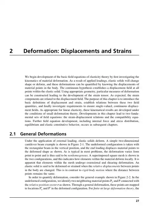
2Deformation:Displacements and Strains We begin development of the basicfield equations of elasticity theory byfirst investigating thekinematics of material deformation.As a result of applied loadings,elastic solids will changeshape or deform,and these deformations can be quantified by knowing the displacements ofmaterial points in the body.The continuum hypothesis establishes a displacementfield at allpoints within the elastic ing appropriate geometry,particular measures of deformationcan be constructed leading to the development of the strain tensor.As expected,the straincomponents are related to the displacementfield.The purpose of this chapter is to introduce thebasic definitions of displacement and strain,establish relations between these twofieldquantities,andfinally investigate requirements to ensure single-valued,continuous displace-mentfields.As appropriate for linear elasticity,these kinematical results are developed underthe conditions of small deformation theory.Developments in this chapter lead to two funda-mental sets offield equations:the strain-displacement relations and the compatibility equa-tions.Furtherfield equation development,including internal force and stress distribution,equilibrium and elastic constitutive behavior,occurs in subsequent chapters.2.1General DeformationsUnder the application of external loading,elastic solids deform.A simple two-dimensionalcantilever beam example is shown in Figure2-1.The undeformed configuration is taken withthe rectangular beam in the vertical position,and the end loading displaces material points tothe deformed shape as shown.As is typical in most problems,the deformation varies frompoint to point and is thus said to be nonhomogenous.A superimposed square mesh is shown inthe two configurations,and this indicates how elements within the material deform locally.It isapparent that elements within the mesh undergo extensional and shearing deformation.Anelastic solid is said to be deformed or strained when the relative displacements between pointsin the body are changed.This is in contrast to rigid-body motion where the distance betweenpoints remains the same.In order to quantify deformation,consider the general example shown in Figure2-2.In the undeformed configuration,we identify two neighboring material points P o and P connected withthe relative position vector r as shown.Through a general deformation,these points are mappedto locations P0and P0in the deformed configuration.Forfinite or large deformation theory,theo27undeformed and deformed configurations can be significantly different,and a distinction between these two configurations must be maintained leading to Lagrangian and Eulerian descriptions;see,for example,Malvern(1969)or Chandrasekharaiah and Debnath(1994). However,since we are developing linear elasticity,which uses only small deformation theory, the distinction between undeformed and deformed configurations can be dropped.Using Cartesian coordinates,define the displacement vectors of points P o and P to be u o and u,respectively.Since P and P o are neighboring points,we can use a Taylor series expansion around point P o to express the components of u asu¼u oþ@u@xr xþ@u@yr yþ@u@zr zv¼v oþ@v@xr xþ@v@yr yþ@v@zr zw¼w oþ@w@xr xþ@w@yr yþ@w@zr z(2:1:1)FIGURE2-1Two-dimensional deformation example.(Undeformed)(Deformed) FIGURE2-2General deformation between two neighboring points.28FOUNDATIONS AND ELEMENTARY APPLICATIONSNote that the higher-order terms of the expansion have been dropped since the components of r are small.The change in the relative position vector r can be written asD r¼r0Àr¼uÀu o(2:1:2) and using(2.1.1)givesD r x¼@u@xr xþ@u@yr yþ@u@zr zD r y¼@v@xr xþ@v@yr yþ@v@zr zD r z¼@w@xr xþ@w@yr yþ@w@zr z(2:1:3)or in index notationD r i¼u i,j r j(2:1:4) The tensor u i,j is called the displacement gradient tensor,and may be written out asu i,j¼@u@x@u@y@u@z@v@x@v@y@v@z@w@x@w@y@w@z2666666437777775(2:1:5)From relation(1.2.10),this tensor can be decomposed into symmetric and antisymmetric parts asu i,j¼e ijþ!ij(2:1:6) wheree ij¼12(u i,jþu j,i)!ij¼12(u i,jÀu j,i)(2:1:7)The tensor e ij is called the strain tensor,while!ij is referred to as the rotation tensor.Relations (2.1.4)and(2.1.6)thus imply that for small deformation theory,the change in the relative position vector between neighboring points can be expressed in terms of a sum of strain and rotation bining relations(2.1.2),(2.1.4),and(2.1.6),and choosing r i¼dx i, we can also write the general result in the formu i¼u o iþe ij dx jþ!ij dx j(2:1:8) Because we are considering a general displacementfield,these results include both strain deformation and rigid-body motion.Recall from Exercise1-14that a dual vector!i canDeformation:Displacements and Strains29be associated with the rotation tensor such that !i ¼À1=2e ijk !jk .Using this definition,it is found that!1¼!32¼12@u 3@x 2À@u 2@x 3 !2¼!13¼12@u 1@x 3À@u 3@x 1 !3¼!21¼12@u 2@x 1À@u 1@x 2 (2:1:9)which can be expressed collectively in vector format as v ¼(1=2)(r Âu ).As is shown in the next section,these components represent rigid-body rotation of material elements about the coordinate axes.These general results indicate that the strain deformation is related to the strain tensor e ij ,which in turn is a related to the displacement gradients.We next pursue a more geometric approach and determine specific connections between the strain tensor components and geometric deformation of material elements.2.2Geometric Construction of Small Deformation TheoryAlthough the previous section developed general relations for small deformation theory,we now wish to establish a more geometrical interpretation of these results.Typically,elasticity variables and equations are field quantities defined at each point in the material continuum.However,particular field equations are often developed by first investigating the behavior of infinitesimal elements (with coordinate boundaries),and then a limiting process is invoked that allows the element to shrink to a point.Thus,consider the common deformational behavior of a rectangular element as shown in Figure 2-3.The usual types of motion include rigid-body rotation and extensional and shearing deformations as illustrated.Rigid-body motion does not contribute to the strain field,and thus also does not affect the stresses.We therefore focus our study primarily on the extensional and shearing deformation.Figure 2-4illustrates the two-dimensional deformation of a rectangular element with original dimensions dx by dy .After deformation,the element takes a rhombus form as shown in the dotted outline.The displacements of various corner reference points areindicated(Rigid Body Rotation)(Undeformed Element)(Horizontal Extension)(Vertical Extension)(Shearing Deformation)FIGURE 2-3Typical deformations of a rectangular element.30FOUNDATIONS AND ELEMENTARY APPLICATIONSin the figure.Reference point A is taken at location (x,y ),and the displacement components of this point are thus u (x,y )and v (x,y ).The corresponding displacements of point B are u (x þdx ,y )and v (x þdx ,y ),and the displacements of the other corner points are defined in an analogous manner.According to small deformation theory,u (x þdx ,y )%u (x ,y )þ(@u =@x )dx ,with similar expansions for all other terms.The normal or extensional strain component in a direction n is defined as the change in length per unit length of fibers oriented in the n -direction.Normal strain is positive if fibers increase in length and negative if the fiber is shortened.In Figure 2-4,the normal strain in the x direction can thus be defined bye x ¼A 0B 0ÀAB From the geometry in Figure 2-4,A 0B 0¼ffiffiffiffiffiffiffiffiffiffiffiffiffiffiffiffiffiffiffiffiffiffiffiffiffiffiffiffiffiffiffiffiffiffiffiffiffiffiffiffiffiffiffiffiffiffiffiffiffiffiffiffiffidx þ@u @x dx 2þ@v @x dx 2s ¼ffiffiffiffiffiffiffiffiffiffiffiffiffiffiffiffiffiffiffiffiffiffiffiffiffiffiffiffiffiffiffiffiffiffiffiffiffiffiffiffiffiffiffiffiffiffiffiffiffiffiffiffiffiffiffiffiffiffiffi1þ2@u @x þ@u @x 2þ@v @x 2dx s %1þ@u @xdx where,consistent with small deformation theory,we have dropped the higher-order ing these results and the fact that AB ¼dx ,the normal strain in the x -direction reduces toe x ¼@u@x (2:2:1)In similar fashion,the normal strain in the y -direction becomese y ¼@v@y (2:2:2)A second type of strain is shearing deformation,which involves angles changes (see Figure 2-3).Shear strain is defined as the change in angle between two originally orthogonalx FIGURE 2-4Two-dimensional geometric strain deformation.Deformation:Displacements and Strains 31directions in the continuum material.This definition is actually referred to as the engineering shear strain.Theory of elasticity applications generally use a tensor formalism that requires a shear strain definition corresponding to one-half the angle change between orthogonal axes; see previous relation(2:1:7)1.Measured in radians,shear strain is positive if the right angle between the positive directions of the two axes decreases.Thus,the sign of the shear strain depends on the coordinate system.In Figure2-4,the engineering shear strain with respect to the x-and y-directions can be defined asg xy¼p2ÀffC0A0B0¼aþbFor small deformations,a%tan a and b%tan b,and the shear strain can then be expressed asg xy¼@v@xdxdxþ@u@xdxþ@u@ydydyþ@v@ydy¼@u@yþ@v@x(2:2:3)where we have again neglected higher-order terms in the displacement gradients.Note that each derivative term is positive if lines AB and AC rotate inward as shown in thefigure.By simple interchange of x and y and u and v,it is apparent that g xy¼g yx.By considering similar behaviors in the y-z and x-z planes,these results can be easily extended to the general three-dimensional case,giving the results:e x¼@u@x,e y¼@v@y,e z¼@w@zg xy¼@u@yþ@v@x,g yz¼@v@zþ@w@y,g zx¼@w@xþ@u@z(2:2:4)Thus,we define three normal and three shearing strain components leading to a total of six independent components that completely describe small deformation theory.This set of equations is normally referred to as the strain-displacement relations.However,these results are written in terms of the engineering strain components,and tensorial elasticity theory prefers to use the strain tensor e ij defined by(2:1:7)1.This represents only a minor change because the normal strains are identical and shearing strains differ by a factor of one-half;for example,e11¼e x¼e x and e12¼e xy¼1=2g xy,and so forth.Therefore,using the strain tensor e ij,the strain-displacement relations can be expressed in component form ase x¼@u@x,e y¼@v@y,e z¼@w@ze xy¼1@uþ@v,e yz¼1@vþ@w,e zx¼1@wþ@u(2:2:5)Using the more compact tensor notation,these relations are written ase ij¼12(u i,jþu j,i)(2:2:6)32FOUNDATIONS AND ELEMENTARY APPLICATIONSwhile in direct vector/matrix notation as the form reads:e¼12r uþ(r u)TÂÃ(2:2:7)where e is the strain matrix and r u is the displacement gradient matrix and(r u)T is its transpose.The strain is a symmetric second-order tensor(e ij¼e ji)and is commonly written in matrix format:e¼[e]¼e x e xy e xze xy e y e yze xz e yz e z2435(2:2:8)Before we conclude this geometric presentation,consider the rigid-body rotation of our two-dimensional element in the x-y plane,as shown in Figure2-5.If the element is rotated through a small rigid-body angular displacement about the z-axis,using the bottom element edge,the rotation angle is determined as@v=@x,while using the left edge,the angle is given byÀ@u=@y. These two expressions are of course the same;that is,@v=@x¼À@u=@y and note that this would imply e xy¼0.The rotation can then be expressed as!z¼[(@v=@x)À(@u=@y)]=2, which matches with the expression given earlier in(2:1:9)3.The other components of rotation follow in an analogous manner.Relations for the constant rotation!z can be integrated to give the result:u*¼u oÀ!z yv*¼v oþ!z x(2:2:9)where u o and v o are arbitrary constant translations in the x-and y-directions.This result then specifies the general form of the displacementfield for two-dimensional rigid-body motion.We can easily verify that the displacementfield given by(2.2.9)yields zero strain.xFIGURE2-5Two-dimensional rigid-body rotation.Deformation:Displacements and Strains33For the three-dimensional case,the most general form of rigid-body displacement can beexpressed asu*¼u oÀ!z yþ!y zv*¼v oÀ!x zþ!z xw*¼w oÀ!y xþ!x y(2:2:10)As shown later,integrating the strain-displacement relations to determine the displacementfield produces arbitrary constants and functions of integration,which are equivalent to rigid-body motion terms of the form given by(2.2.9)or(2.2.10).Thus,it is important to recognizesuch terms because we normally want to drop them from the analysis since they do notcontribute to the strain or stressfields.2.3Strain TransformationBecause the strains are components of a second-order tensor,the transformation theorydiscussed in Section1.5can be applied.Transformation relation(1:5:1)3is applicable forsecond-order tensors,and applying this to the strain givese0ij¼Q ip Q jq e pq(2:3:1)where the rotation matrix Q ij¼cos(x0i,x j).Thus,given the strain in one coordinate system,we can determine the new components in any other rotated system.For the general three-dimensional case,define the rotation matrix asQ ij¼l1m1n1l2m2n2l3m3n32435(2:3:2)Using this notational scheme,the specific transformation relations from equation(2.3.1)becomee0x¼e x l21þe y m21þe z n21þ2(e xy l1m1þe yz m1n1þe zx n1l1)e0y¼e x l22þe y m22þe z n22þ2(e xy l2m2þe yz m2n2þe zx n2l2)e0z¼e x l23þe y m23þe z n23þ2(e xy l3m3þe yz m3n3þe zx n3l3)e0xy¼e x l1l2þe y m1m2þe z n1n2þe xy(l1m2þm1l2)þe yz(m1n2þn1m2)þe zx(n1l2þl1n2)e0yz¼e x l2l3þe y m2m3þe z n2n3þe xy(l2m3þm2l3)þe yz(m2n3þn2m3)þe zx(n2l3þl2n3)e0zx¼e x l3l1þe y m3m1þe z n3n1þe xy(l3m1þm3l1)þe yz(m3n1þn3m1)þe zx(n3l1þl3n1)(2:3:3)For the two-dimensional case shown in Figure2-6,the transformation matrix can be ex-pressed asQ ij¼cos y sin y0Àsin y cos y00012435(2:3:4)34FOUNDATIONS AND ELEMENTARY APPLICATIONSUnder this transformation,the in-plane strain components transform according toe 0x ¼e x cos 2y þe y sin 2y þ2e xy sin y cos ye 0y ¼e x sin 2y þe y cos 2y À2e xy sin y cos ye 0xy ¼Àe x sin y cos y þe y sin y cos y þe xy (cos 2y Àsin 2y )(2:3:5)which is commonly rewritten in terms of the double angle:e 0x ¼e x þe y 2þe x Àe y 2cos 2y þe xy sin 2y e 0y ¼e x þe y Àe x Àe y cos 2y Àe xy sin 2y e 0xy ¼e y Àe x 2sin 2y þe xy cos 2y (2:3:6)Transformation relations (2.3.6)can be directly applied to establish transformations between Cartesian and polar coordinate systems (see Exercise 2-6).Additional applications of these results can be found when dealing with experimental strain gage measurement systems.For example,standard experimental methods using a rosette strain gage allow the determination of extensional strains in three different directions on the surface of a ing this type of data,relation (2:3:6)1can be repeatedly used to establish three independent equations that can be solved for the state of strain (e x ,e y ,e xy )at the surface point under study (see Exercise 2-7).Both two-and three-dimensional transformation equations can be easily incorporated in MATLAB to provide numerical solutions to problems of interest.Such examples are given in Exercises 2-8and 2-9.2.4Principal StrainsFrom the previous discussion in Section 1.6,it follows that because the strain is a symmetric second-order tensor,we can identify and determine its principal axes and values.According to this theory,for any given strain tensor we can establish the principal value problem and solvey ′FIGURE 2-6Two-dimensional rotational transformation.Deformation:Displacements and Strains 35the characteristic equation to explicitly determine the principal values and directions.The general characteristic equation for the strain tensor can be written asdet[e ijÀe d ij]¼Àe3þW1e2ÀW2eþW3¼0(2:4:1) where e is the principal strain and the fundamental invariants of the strain tensor can be expressed in terms of the three principal strains e1,e2,e3asW1¼e1þe2þe3W2¼e1e2þe2e3þe3e1W3¼e1e2e3(2:4:2)Thefirst invariant W1¼W is normally called the cubical dilatation,because it is related to the change in volume of material elements(see Exercise2-11).The strain matrix in the principal coordinate system takes the special diagonal forme ij¼e1000e2000e32435(2:4:3)Notice that for this principal coordinate system,the deformation does not produce anyshearing and thus is only extensional.Therefore,a rectangular element oriented alongprincipal axes of strain will retain its orthogonal shape and undergo only extensional deform-ation of its sides.2.5Spherical and Deviatoric StrainsIn particular applications it is convenient to decompose the strain tensor into two parts calledspherical and deviatoric strain tensors.The spherical strain is defined by~e ij¼13e kk d ij¼13Wd ij(2:5:1)while the deviatoric strain is specified as^e ij¼e ijÀ13e kk d ij(2:5:2)Note that the total strain is then simply the sume ij¼~e ijþ^e ij(2:5:3)The spherical strain represents only volumetric deformation and is an isotropic tensor,being the same in all coordinate systems(as per the discussion in Section1.5).The deviatoricstrain tensor then accounts for changes in shape of material elements.It can be shownthat the principal directions of the deviatoric strain are the same as those of the straintensor.36FOUNDATIONS AND ELEMENTARY APPLICATIONS2.6Strain CompatibilityWe now investigate in more detail the nature of the strain-displacement relations (2.2.5),and this will lead to the development of some additional relations necessary to ensure continuous,single-valued displacement field solutions.Relations (2.2.5),or the index notation form (2.2.6),represent six equations for the six strain components in terms of three displacements.If we specify continuous,single-valued displacements u,v,w,then through differentiation the resulting strain field will be equally well behaved.However,the converse is not necessarily true;that is,given the six strain components,integration of the strain-displacement relations (2.2.5)does not necessarily produce continuous,single-valued displacements.This should not be totally surprising since we are trying to solve six equations for only three unknown displacement components.In order to ensure continuous,single-valued displacements,the strains must satisfy additional relations called integrability or compatibility equations .Before we proceed with the mathematics to develop these equations,it is instructive to consider a geometric interpretation of this concept.A two-dimensional example is shown in Figure 2-7whereby an elastic solid is first divided into a series of elements in case (a).For simple visualization,consider only four such elements.In the undeformed configuration shown in case (b),these elements of course fit together perfectly.Next,let us arbitrarily specify the strain of each of the four elements and attempt to reconstruct the solid.For case (c),the elements have been carefully strained,taking into consideration neighboring elements so that the system fits together thus yielding continuous,single-valued displacements.However,for(b) Undeformed Configuration(c) Deformed ConfigurationContinuous Displacements (a) Discretized Elastic Solid (d) Deformed Configuration Discontinuous DisplacementsFIGURE 2-7Physical interpretation of strain compatibility.case(d),the elements have been individually deformed without any concern for neighboring deformations.It is observed for this case that the system will notfit together without voids and gaps,and this situation produces a discontinuous displacementfield.So,we again conclude that the strain components must be somehow related to yield continuous,single-valued displacements.We now pursue these particular relations.The process to develop these equations is based on eliminating the displacements from the strain-displacement relations.Working in index notation,we start by differentiating(2.2.6) twice with respect to x k and x l:e ij,kl¼12(u i,jklþu j,ikl)Through simple interchange of subscripts,we can generate the following additional relations:e kl,ij¼12(u k,lijþu l,kij)e jl,ik¼12(u j,likþu l,jik)e ik,jl¼12(u i,kjlþu k,ijl)Working under the assumption of continuous displacements,we can interchange the order of differentiation on u,and the displacements can be eliminated from the preceding set to gete ij,klþe kl,ijÀe ik,jlÀe jl,ik¼0(2:6:1) These are called the Saint Venant compatibility equations.Although the system would lead to 81individual equations,most are either simple identities or repetitions,and only6are meaningful.These six relations may be determined by letting k¼l,and in scalar notation, they become@2e x @y2þ@2e y@x2¼2@2e xy@x@y@2e y @z2þ@2e z@y2¼2@2e yz@y@z@2e z @x2þ@2e x@z2¼2@2e zx@z@x@2e x @y@z ¼@@xÀ@e yz@xþ@e zx@yþ@e xy@z@2e y @z@x ¼@@yÀ@e zx@yþ@e xy@zþ@e yz@x@2e z @x@y ¼@@zÀ@e xy@zþ@e yz@xþ@e zx@y(2:6:2)It can be shown that these six equations are equivalent to three independent fourth-order relations(see Exercise2-14).However,it is usually more convenient to use the six second-order equations given by(2.6.2).In the development of the compatibility relations,we assumed that the displacements were continuous,and thus the resulting equations (2.6.2)are actually only a necessary condition.In order to show that they are also sufficient,consider two arbitrary points P and P o in an elastic solid,as shown in Figure 2-8.Without loss in generality,the origin may be placed at point P o .The displacements of points P and P o are denoted by u P i and u o i ,and the displacement ofpoint P can be expressed asu P i ¼u o i þðC du i ¼u o i þðC @u i @x j dx j (2:6:3)where C is any continuous curve connecting points P o and P .Using relation (2.1.6)for the displacement gradient,(2.6.3)becomesu P i ¼u o i þðC (e ij þ!ij )dx j (2:6:4)Integrating the last term by parts givesðC !ij dx j ¼!P ij x P j ÀðC x j !ij ,k dx k (2:6:5)where !P ij is the rotation tensor at point P .Using relation (2:1:7)2,!ij ,k ¼12(u i ,jk Àu j ,ik )¼12(u i ,jk Àu j ,ik )þ12(u k ,ji Àu k ,ji )¼12@@x j (u i ,k þu k ,i )À12@@x i(u j ,k þu k ,j )¼e ik ,j Àe jk ,i (2:6:6)Substituting results (2.6.5)and (2.6.6)into (2.6.4)yieldsu P i¼u o i þ!P ij x P j þðC U ik dx k (2:6:7)where U ik ¼e ik Àx j (e ik ,j Àe jk ,i ).P oFIGURE 2-8Continuity of displacements.Now if the displacements are to be continuous,single-valued functions,the line integral appearing in(2.6.7)must be the same for any curve C;that is,the integral must be independent of the path of integration.This implies that the integrand must be an exact differential,so that the value of the integral depends only on the end points.Invoking Stokes theorem,we can show that if the region is simply connected(definition of the term simply connected is postponed for the moment),a necessary and sufficient condition for the integral to be path independent is for U ik,l¼U il,ing this result yieldse ik,lÀd jl(e ik,jÀe jk,i)Àx j(e ik,jlÀe jk,il)¼e il,kÀd jk(e il,jÀe jl,i)Àx j(e il,jkÀe jl,ik) which reduces tox j(e ik,jlÀe jk,ilÀe il,jkþe jl,ik)¼0Because this equation must be true for all values of x j,the terms in parentheses must vanish, and after some index renaming this gives the identical result previously stated by the compati-bility relations(2.6.1):e ij,klþe kl,ijÀe ik,jlÀe jl,ik¼0Thus,relations(2.6.1)or(2.6.2)are the necessary and sufficient conditions for continuous, single-valued displacements in simply connected regions.Now let us get back to the term simply connected.This concept is related to the topology or geometry of the region under study.There are several places in elasticity theory where the connectivity of the region fundamentally affects the formulation and solution method. The term simply connected refers to regions of space for which all simple closed curves drawn in the region can be continuously shrunk to a point without going outside the region. Domains not having this property are called multiply connected.Several examples of such regions are illustrated in Figure2-9.A general simply connected two-dimensional region is shown in case(a),and clearly this case allows any contour within the region to be shrunk to a point without going out of the domain.However,if we create a hole in the region as shown in case(b),a closed contour surrounding the hole cannot be shrunk to a point without going into the hole and thus outside of the region.Thus,for two-dimensional regions,the presence of one or more holes makes the region multiply connected.Note that by introducing a cut between the outer and inner boundaries in case(b),a new region is created that is now simply connected. Thus,multiply connected regions can be made simply connected by introducing one or more cuts between appropriate boundaries.Case(c)illustrates a simply connected three-dimensional example of a solid circular cylinder.If a spherical cavity is placed inside this cylinder as shown in case(d),the region is still simply connected because any closed contour can still be shrunk to a point by sliding around the interior cavity.However,if the cylinder has a through hole as shown in case(e),then an interior contour encircling the axial through hole cannot be reduced to a point without going into the hole and outside the body.Thus,case(e)is an example of the multiply connected three-dimensional region.It was found that the compatibility equations are necessary and sufficient conditions for continuous,single-valued displacements only for simply connected regions.However, for multiply connected domains,relations(2.6.1)or(2.6.2)provide only necessary but。
材料力学双语教学学习资料第一章绪论Chapter 1 Introduction§1-1 材料力学的任务The Tasks of Mechanics of Materials1*. 材料力学: Mechanics of Materials2. 构件: Structural Members3. 变形: Deformation4*. 强度: Strength5*. 刚度: Rigidity6*. 稳定性: Stability§1-2 变形固体的基本假设Fundamental Assumptions of SolidDeformation Bodies1. 连续性假设: Continuity2. 均匀性假设: Homogeneity3. 各向同性假设: Isotropy§1.3 外力及其分类External Forces and Classification1. 分布力: Distributed Force2. 集中力: Point Force3. 静载荷: Static Load4. 动载荷: Dynamic Load§1.4 内力、截面法和应力的概念Concepts of Internal Forces,Method ofSection and Stress1*. 内力: Internal Force2*. 截面法: Method of Section3. 截面法的三个步骤:截开,代替,平衡Three steps of method of section: cut off, substitute , and equilibrium.4*. 应力: Stress5. 平均应力:Average stress6. 应力(全应力):Whole stress(sum stress)7*. 正应力: Normal Stress8*. 剪应力(切应力):Shearing Stress§1.5 变形与应变Deformation and Strain1.线应变: Strain2.剪应变: Shearing Strain§1.6 杆件变形的基本形式Basic Types of Deformations of Rods1*. 拉伸或压缩: Tension or Compression2*. 剪切: Shear3*. 扭转: Torsion4*. 弯曲: Bending第二章拉伸、压缩与剪切Chapter 2 Tension,Compression andShear§2.1 轴向拉伸与压缩的概念和实例The Concept and Examples of AxialTension and Compression1. 拉杆: Tensile Rod2. 压杆: Compressive Rod3. 受力特点:外力合力的作用线与杆轴线重合Characteristic of the External Forces: The acting line of the resultant of external forces is coincided with the axis of the rod.4. 变形特点:杆沿轴向伸长或缩短Characteristic of Deformation: Rod will elongate or contract along the axis of the rod.§2.2 轴向拉伸或压缩时横截面上的内力和应力Internal Force and Stress of Axial Tension or Compression on the Cross Section1*. 横截面: Cross Section2*. 轴力: Normal Force3*. 轴力图: Diagram of Normal Force§2.3 直杆轴向拉伸或压缩时斜截面上的应力Stress of Axial Tension or Compressionon the Skew Section1. 斜截面: Skew Section2.ασσα2cos = αστα2s i n 2=§2.4 材料在拉伸时的力学性能Mechanical Properties of Materialswith Tensile Load1. 标准试件: Specimen2. 低碳钢(C ≤0.3%): Low Carbon Steel3. 弹性阶段:Elastic Region4. 屈服阶段:Yielding Stage5. 强化阶段:Hardening Stage6. 颈缩阶段: Necking Stage 7*.σp ----比例极限: Proportional Limit 8*.σe ----弹性极限: Elastic Limit 9*.σs ----屈服极限: Yielding Stress 10*.σb ----强度极限: Ultimate Stress 11. 延伸率: Percent Elongation12. 断面收缩率: Percent Reduction of Area 13. 塑性材料: Ductile Materials 14. 脆性材料: Brittle Materials 15. 铸铁:Cast iron§2.7 失效、安全系数和强度计算 Failure, Safety factor and Strengthcalculation1*. 许用应力: Allowable Stress 2. 安全系数: Safety Factor 3*. 强度条件: Strength Condition][max σσ≤=AF N4*. 强度校核: Check strength][max σσ≤5*. 截面设计: Section design][σNF A ≥6*. 确定许可载荷:Determine allowable load][σA F N ≤§2.8 轴向拉伸或压缩时的变形 Deformation in Axial Tension orCompression1. 弹性变形: Elastic Deformation2. 塑性变形: Plastic Deformation3. 纵向应变: Longitudinal Strainll l l l -=∆=1ε 4. 横向应变: Lateral Straindd d d d -=∆=''ε5.线弹性变形:Linear Elastic Deformation6.泊松比:Poisson’s ratioεεμ'=7*.弹性模量-E :表示材料抵抗拉压变形的 能力 E - modulus of elasticity :Indicates the capability of materials for resisting tension or compression 8*.抗拉刚度-EA :表示构件抵抗拉压变形的能力EA -the axial rigidity: Indicates the capability of constructive members for resisting tension or compression 9*. 胡克定律(Hooke’s Law ):当应力不超过材料的比例极限时,应力与应变成正比.The stress is proportional to the strain within the elastic region.εσE =§2.12 应力集中的概念The Concept of Stress Concentration 1.由于截面尺寸的突然变化,使截面上的应力分布不再均匀,在某些部位出现远大于平均值的应力,称应力集中。