ACM2004-On Clusterings Good Bad and Spectral
- 格式:pdf
- 大小:166.81 KB
- 文档页数:19


求余运算给出S和M,求0*S%M,1*S%M,2*S%M......(M-1)*S%M能否组成一个集合包含0.1.。
M-1;(这个是原题意改造而来);算法:判断两个数是否互质;or 暴力解决其实暴力完全可以解决这个问题(⊙﹏⊙b),只是其中用数学方法更加高效,巧妙;证明如果S和M互质则满足题意:另G=gcd(S,M);则S=A*G,M=B*G;另X=K*S%M=K*S-T*M(T为整数,满足X属于0到M-1);X=K*A*G-T*B*G;因此取余后的整数一定是G的倍数,G只能取1才能满足条件;充分性的证明:(即当S与M互质,则0到M-1的S倍对M取余一定能遍历0到M-1)只需证明的是,该余数中两两之间互不相等;假设k*S和b*S对M取余相等(k和b∈[0,M),并且k和b不等);则k*S=q1*M+r=q2*M+r=b*S <==> (k-b)*S=M*(q1-q2);S与M互质,由上式子可得M|(k-b),与k和b∈[0,M),并且k和b不等矛盾;因此得证;另外,偶然看到一个很牛叉的辗转相除法;int gcd(int a,int b){while(b) b^=a^=b^=a%=b;return a;}此代码,很好很强大;把涉及位运算的交换的程序加入,便到得这段简洁高效的代码;注:A和B;经过A^=B^=A^=B,结果就得到A和B的交换//////////////////////////// 1000#include <stdio.h>int main(){int a,b,i,;scanf("%d",&a);for(i=1;i<=a;i++){ int sum=0;sum=sum+i;printf("%d\n",sum);}return 0;};1001;#include"stdio.h"int main(){unsigned _int64 n;unsigned _int64 temp;while(scanf("%I64u",&n)!=EOF) //是i 非L{temp=(1+n)*n/2;printf("%I64u\n\n",temp);}return 0;}//////////////////HDU ACM 1014 Uniform Generator 三月22nd, /showproblem.php?pid=1014这个题目是判断给定的步长和mod,判断所产生的随机数已经覆盖0~mod-1中所有的数,如果是,则说明所选的步长和mod是一个Good choice,否则为bad choice.需要懂得的基本内容为线性同余产生随机数,链接:/zh-cn/%E7%B7%9A%E6%80%A7%E5%90%8C%E9%A4%98%E6%96 %B9%E6%B3%95Problem DescriptionComputer simulations often require random numbers. One way to generate pseudo-random numbers is via a function of the formseed(x+1) = [seed(x) + STEP] % MODwhere '%' is the modulus operator.Such a function will generate pseudo-random numbers (seed) between 0 and MOD-1. One problem with functions of this form is that they will always generate the same pattern over and over. In order to minimize this effect, selecting the STEP and MOD values carefully can result in a uniform distribution of all values between (and including) 0 and MOD-1.For example, if STEP = 3 and MOD = 5, the function will generate the series of pseudo-random numbers 0, 3, 1, 4, 2 in a repeating cycle. In this example, all of the numbers between and including 0 and MOD-1 will be generated every MOD iterations of the function. Note that by the nature of the function to generate the same seed(x+1) every time seed(x) occurs means that if a function will generate all the numbers between 0 and MOD-1, it will generate pseudo-random numbers uniformly with every MOD iterations.If STEP = 15 and MOD = 20, the function generates the series 0, 15, 10, 5 (or any other repeating series if the initial seed is other than 0). This is a poor selection of STEP and MOD because no initial seed will generate all of the numbers from 0 and MOD-1.Your program will determine if choices of STEP and MOD will generate a uniform distribution of pseudo-random numbers.InputEach line of input will contain a pair of integers for STEP and MOD in that order (1 <= STEP, MOD <= 100000).OutputFor each line of input, your program should print the STEP value right- justified in columns 1 through 10, the MOD value right-justified in columns 11 through 20 and either "Good Choice" or "Bad Choice" left-justified starting in column 25. The "Good Choice" message should be printed when the selection of STEP and MOD will generate all the numbers between and including 0 and MOD-1 when MOD numbers are generated. Otherwise, your program should print the message "Bad Choice". After each output test set, your program should print exactly one blank line.Sample Input3 515 2063923 99999Sample Output3 5 Good Choice15 20 Bad Choice63923 99999 Good Choice线性同余方法(LCG)是个产生伪随机数的方法。
Screened Poisson Surface ReconstructionMICHAEL KAZHDANJohns Hopkins UniversityandHUGUES HOPPEMicrosoft ResearchPoisson surface reconstruction creates watertight surfaces from oriented point sets.In this work we extend the technique to explicitly incorporate the points as interpolation constraints.The extension can be interpreted as a generalization of the underlying mathematical framework to a screened Poisson equation.In contrast to other image and geometry processing techniques,the screening term is defined over a sparse set of points rather than over the full domain.We show that these sparse constraints can nonetheless be integrated efficiently.Because the modified linear system retains the samefinite-element discretization,the sparsity structure is unchanged,and the system can still be solved using a multigrid approach. Moreover we present several algorithmic improvements that together reduce the time complexity of the solver to linear in the number of points, thereby enabling faster,higher-quality surface reconstructions.Categories and Subject Descriptors:I.3.5[Computer Graphics]:Compu-tational Geometry and Object ModelingAdditional Key Words and Phrases:screened Poisson equation,adaptive octree,finite elements,surfacefittingACM Reference Format:Kazhdan,M.,and Hoppe,H.Screened Poisson surface reconstruction. ACM Trans.Graph.NN,N,Article NN(Month YYYY),PP pages.DOI=10.1145/XXXXXXX.YYYYYYY/10.1145/XXXXXXX.YYYYYYY1.INTRODUCTIONPoisson surface reconstruction[Kazhdan et al.2006]is a well known technique for creating watertight surfaces from oriented point samples acquired with3D range scanners.The technique is resilient to noisy data and misregistration artifacts.However, as noted by several researchers,it suffers from a tendency to over-smooth the data[Alliez et al.2007;Manson et al.2008; Calakli and Taubin2011;Berger et al.2011;Digne et al.2011].In this work,we explore modifying the Poisson reconstruc-tion algorithm to incorporate positional constraints.This mod-ification is inspired by the recent reconstruction technique of Calakli and Taubin[2011].It also relates to recent work in im-age and geometry processing[Nehab et al.2005;Bhat et al.2008; Chuang and Kazhdan2011],in which a datafidelity term is used to“screen”the associated Poisson equation.In our surface recon-struction context,this screening term corresponds to a soft con-straint that encourages the reconstructed isosurface to pass through the input points.The approach we propose differs from the traditional screened Poisson formulation in that the position and gradient constraints are defined over different domain types.Whereas gradients are constrained over the full3D space,positional constraints are introduced only over the input points,which lie near a2D manifold. We show how these two types of constraints can be efficiently integrated,so that we can leverage the original multigrid structure to solve the linear system without incurring a significant overhead in space or time.To demonstrate the benefits of screening,Figure1compares results of the traditional Poisson surface reconstruction and the screened Poisson formulation on a subset of11.4M points from the scan of Michelangelo’s David[Levoy et al.2000].Both reconstructions are computed over a spatial octree of depth10,corresponding to an effective voxel resolution of10243.Screening generates a model that better captures the input data(as visualized by the surface cross-sections overlaid with the projection of nearby samples), even though both reconstructions have similar complexity(6.8M and6.9M triangles respectively)and required similar processing time(230and272seconds respectively,without parallelization).1 Another contribution of our work is to modify both the octree structure and the multigrid implementation to reduce the time complexity of solving the Poisson system from log-linear to linear in the number of input points.Moreover we show that hierarchical point clustering enables screened Poisson reconstruction to attain this same linear complexity.2.RELA TED WORKReconstructing surfaces from scanned points is an important and extensively studied problem in computer graphics.The numerous approaches can be broadly categorized as follows. Combinatorial Algorithms.Many schemes form a triangula-tion using a subset of the input points[Cazals and Giesen2006]. Space is often discretized using a tetrahedralization or a voxel grid,and the resulting elements are partitioned into inside and outside regions using an analysis of cells[Amenta et al.2001; Boissonnat and Oudot2005;Podolak and Rusinkiewicz2005], eigenvector computation[Kolluri et al.2004],or graph cut [Labatut et al.2009;Hornung and Kobbelt2006].Implicit Functions.In the presence of sampling noise,a common approach is tofit the points using the zero set of an implicit func-tion,such as a sum of radial bases[Carr et al.2001]or piecewise polynomial functions[Ohtake et al.2005;Nagai et al.2009].Many techniques estimate a signed-distance function[Hoppe et al.1992; 1The performance of the unscreened solver is measured using our imple-mentation with screening weight set to zero.The implementation of the original Poisson reconstruction runs in412seconds.ACM Transactions on Graphics,V ol.VV,No.N,Article XXX,Publication date:Month YYYY.2•M.Kazhdan and H.HoppeFig.1:Reconstruction of the David head ‡,comparing traditional Poisson surface reconstruction (left)and screened Poisson surface reconstruction which incorporates point constraints (center).The rightmost diagram plots pixel depth (z )values along the colored segments together with the positions of nearby samples.The introduction of point constraints significantly improves fit accuracy,sharpening the reconstruction without amplifying noise.Bajaj et al.1995;Curless and Levoy 1996].If the input points are unoriented,an important step is to correctly infer the sign of the resulting distance field [Mullen et al.2010].Our work extends Poisson surface reconstruction [Kazhdan et al.2006],in which the implicit function corresponds to the model’s indicator function χ.The function χis often defined to have value 1inside and value 0outside the model.To simplify the derivations,inthis paper we define χto be 12inside and −12outside,so that its zero isosurface passes near the points.The function χis solved using a Laplacian system discretized over a multiresolution B-spline basis,as reviewed in Section 3.Alliez et al.[2007]form a Laplacian system over a tetrahedral-ization,and constrain the solution’s biharmonic energy;the de-sired function is obtained as the solution to an eigenvector prob-lem.Manson et al.[2008]represent the indicator function χusing a wavelet basis,and efficiently compute the basis coefficients using simple local sums over an adapted octree.Calakli and Taubin [2011]optimize a signed-distance function to have value zero at the points,have derivatives that agree with the point normals,and minimize a Hessian smoothness norm.The resulting optimization involves a bilaplacian operator,which requires estimating derivatives of higher order than in the Laplacian.The reconstructed surfaces are shown to have good accuracy,strongly suggesting the importance of explicitly fitting the points within the optimization.This motivated us to explore whether a Laplacian system could be extended in this respect,and also be compatible with a multigrid solver.Screened Poisson Surface Fitting.The method of Nehab et al.[2005],which simultaneously fits position and normal constraints,may also be viewed as the solution of a screened Poisson equation.The fitting algorithm assumes that a 2D parametric domain (i.e.,a plane or triangle mesh)is already established.The position and derivative constraints are both defined over this 2D domain.In contrast,in Poisson surface reconstruction the 2D domain manifold is initially unknown,and therefore the goal is to infer anindicator function χrather than a parametric function.This leadsto a hybrid problem with derivative (Laplacian)constraints defined densely over 3D and position constraints defined sparsely on the set of points sampled near the unknown 2D manifold.3.REVIEW OF POISSON SURFACE RECONSTRUCTIONThe approach of Poisson surface reconstruction is based on the observation that the (inward pointing)normal field of the boundary of a solid can be interpreted as the gradient of the solid’s indicator function.Thus,given a set of oriented points sampling the boundary,a watertight mesh can be obtained by (1)transforming the oriented point samples into a continuous vector field in 3D,(2)finding a scalar function whose gradients best match the vector field,and (3)extracting the appropriate isosurface.Because our work focuses primarily on the second step,we review it here in more detail.Scalar Function Fitting.Given a vector field V :R 3→R 3,thegoal is to solve for the scalar function χ:R 3→R minimizing:E (χ)=∇χ(p )− V (p ) 2d p .(1)Using the Euler-Lagrange formulation,the minimum is obtainedby solving the Poisson equation:∆χ=∇· V .System Discretization.The Galerkin formulation is used totransform this into a finite-dimensional system [Fletcher 1984].First,a basis {B 1,...,B N }:R 3→R is chosen,namely a collection of trivariate (usually triquadratic)B-spline functions.With respect to this basis,the discretization becomes:∆χ,B i [0,1]3= ∇· V ,B i [0,1]31≤i ≤Nwhere ·,· [0,1]3is the standard inner-product on the space of(scalar-and vector-valued)functions defined on the unit cube:F ,G [0,1]3=[0,1]3F (p )·G (p )d p , U , V [0,1]3=[0,1]3U (p ), V (p ) d p .Since the solution is itself expressed in terms of the basis functions:χ(p )=N∑i =1x i B i (p ),ACM Transactions on Graphics,V ol.VV ,No.N,Article XXX,Publication date:Month YYYY .1.离散化->连续2.找个常量函数最佳拟合这些这些向量域;3.抽取等值面这里已经将离散的有向点转化为了连续的向量域表示;点集合的最初的思考Screened Poisson Surface Reconstruction•3finding the coefficients{x i}of the solution reduces to solving the linear system Ax=b where:A i j= ∇B i,∇B j [0,1]3and b i= V,∇B i [0,1]3.(2) The basis functions{B1,...,B N}are chosen to be compactly supported,so most pairs of functions do not have overlapping support,and thus the matrix A is sparse.Because the solution is expected to be smooth away from the input samples,the linear system is discretized byfirst adapting an octree to the input samples and then associating an(appropriately scaled and translated)trivariate B-spline function to each octree node. This provides high-resolution detail in the vicinity of the surface while reducing the overall dimensionality of the system.System Solution.Given the hierarchy defined by an octree of depth D,a multigrid approach is used to solve the linear system. The basis functions are partitioned according to the depths of their associated nodes and,for each depth d,a linear system A d x d=b d is defined using the corresponding B-splines{B d1,...,B d Nd},such thatχ(p)=∑D d=0∑i x d i B d i(p).Because the octree-selected B-spline functions do not form a complete grid at each depth,it is generally not possible to prolong the solution x d at depth d into the solution x d+1at depth d+1. (The B-spline associated with a given node is a sum of B-spline functions associated not only with its own child nodes,but also with child nodes of its neighbors.)Instead,the constraints at depth d+1are adjusted to account for the part of the solution already realized at coarser depths.Pseudocode for a cascadic solver,where the solution is only relaxed on the up-stroke of the V-cycle,is given in Algorithm1.Algorithm1:Cascadic Poisson Solver1For d∈{0,...,D}Iterate from coarse tofine2For d ∈{0,...,d−1}Remove the constraints3b d=b d−A dd x d met at coarser depths4Relax A d x d=b d Adjust the system at depth dHere,A dd is the N d×N d matrix used to transform solution coefficients at depth d into constraints at depth d:A dd i j= ∇B d i,∇B d j [0,1]3.Note that,by definition,A d=A dd.Isosurface Extraction.Solving the Poisson equation,one obtains a functionχthat approximates the indicator function.Ideally,the function’s zero level-set should therefore correspond to the desired surface.In practice however,the functionχcan differ from the true indicator function due to several sources of error:—The point sampling may be noisy,possibly containing outliers.—The Galerkin discretization is only an approximation of the continuous problem.—The point sampling density is approximated during octree construction.To mitigate these errors,in[Kazhdan et al.2006]the implicit function is adjusted by globally subtracting the average value of the function at the input samples.4.INCORPORA TING POINT CONSTRAINTSThe original Poisson surface reconstruction algorithm adjusts the implicit function using a single global offset such that its average value at all points is zero.However,the presence of errors can cause the implicit function to drift so that no global offset is satisfactory. Instead,we seek to explicitly interpolate the points.Given the set of input points P with weights w:P→R≥0,we add to the energy of Equation1a term that penalizes the function’s deviation from zero at the samples:E(χ)=V(p)−∇χ(p) 2d p+α·Area(P)∑p∈P∑p∈Pw(p)χ2(p)(3)whereαis a weight that trades off the importance offitting the gradients andfitting the values,and Area(P)is the area of the reconstructed surface,estimated by computing the local sampling density as in[Kazhdan et al.2006].In our implementation,we set the per-sample weights w(p)=1,although one can also use confidence values if these are available.The energy can be expressed concisely asE(χ)= V−∇χ, V−∇χ [0,1]3+α χ,χ (w,P)(4)where ·,· (w,P)is the bilinear,symmetric,positive,semi-definite form on the space of functions in the unit-cube,obtained by taking the weighted sum of function values:F,G (w,P)=Area(P)∑p∈P w(p)∑p∈Pw(p)·F(p)·G(p).4.1Interpretation as a Screened Poisson EquationThe energy in Equation4combines a gradient constraint integrated over the spatial domain with a value constraint summed at discrete points.As shown in the appendix,its minimization can be interpreted as a screened Poisson equation(∆−α˜I)χ=∇· V with an appropriately defined operator˜I.4.2DiscretizationWe apply a discretization similar to that in Section3to the minimization of the energy in Equation4.The coefficients of the solutionχwith respect to the basis{B1,...,B N}are again obtained by solving a linear system of the form Ax=b.The right-hand-side b is unchanged because the constrained value at the sample points is zero.Matrix A now includes the point constraints:A i j= ∇B i,∇B j [0,1]3+α B i,B j (w,P).(5) Note that incorporating the point constraints does not change the sparsity of matrix A because B i(p)·B j(p)is nonzero only if the supports of the two functions overlap,in which case the Poisson equation has already introduced a nonzero entry in the matrix.As in Section3,we solve this linear system using a cascadic multigrid algorithm–iterating over the octree depths from coarsest tofinest,adjusting the constraints,and relaxing the system.Similar to Equation5,the matrix used to transform a solution at depth d to a constraint at depth d is expressed as:A dd i j= ∇B d i,∇B d j [0,1]3+α B d i,B d j (w,P).ACM Transactions on Graphics,V ol.VV,No.N,Article XXX,Publication date:Month YYYY.4•M.Kazhdan and H.HoppeFig.2:Visualizations of the reconstructed implicit function along a planar slice through the cow ‡(shown in blue on the left),for the original Poisson solver,and for the screened Poisson solver without and with scale-independent screening.This operator adjusts the constraint b d (line 3of Algorithm 1)not only by removing the Poisson constraints met at coarser resolutions,but also by modifying the constrained values at points where the coarser solution does not evaluate to zero.4.3Scale-Independent ScreeningTo balance the two energy terms in Equation 3,it is desirable to adjust the screening parameter αsuch that (1)the reconstructed surface shape is invariant under scaling of the input points with respect to the solver domain,and (2)the prolongation of a solution at a coarse depth is an accurate estimate of the solution at a finer depth in the cascadic multigrid approach.We achieve both these goals by adjusting the relative weighting of position and gradient constraints across the different octree depths.Noting that the magnitude of the gradient constraint scales with resolution,we double the weight of the interpolation constraint with each depth:A ddi j = ∇B d i ,∇B dj [0,1]3+2d α B d i ,B dj (w ,P ).The adaptive weight of 2d is chosen to keep the Laplacian and screening constraints around the surface in balance.To see this,assume that the points are locally planar,and consider the row of the system matrix corresponding to an octree node overlapping the points.The coefficients of the system in that row are the sum of Laplacian and screening terms.If we consider the rows corresponding to the child nodes that overlap the surface,we find that the contribution from the Laplacian constraints scales by a factor of 1/2while the contribution from the screening term scales by a factor of 1/4.2Thus,scaling the screening weights by a factor of two with each resolution keeps the two terms in balance.Figure 2shows the benefit of scale-independent screening in reconstructing a cow model.The leftmost image shows a plane passing through the bounding cube of the cow,and the images to the right show the values of the computed indicator function along that plane,for different implementations of the solver.As the figure shows,the unscreened Poisson solver provides a good approximation of the indicator functions,with values inside (resp.outside)the surface approximately 1/2(resp.-1/2).However,applying the same solver to the screened Poisson equation (second from right)provides a solution that is only correct near the input samples and returns to zero near the faces of the bounding cube,2Forthe Laplacian term,the Laplacian scales by a factor of 4with refinement,and volumetric integrals scale by a factor of 1/8.For the screening term,area integrals scale by a factor of 1/4.potentially resulting in spurious surface sheets away from the surface.It is only with scale-independent screening (right)that we obtain a high-quality solution to the screened Poisson ing this resolution adaptive weighting,our system has the property that the reconstruction obtained by solving at depth D is identical to the reconstruction that would be obtained by scaling the point set by 1/2and solving at depth D +1.To see this,we consider the two energies that guide the reconstruc-tion,E V (χ)measuring the extent to which the gradients of the so-lution match the prescribed vector field,and E (w ,P )(χ)measuring the extent to which the solution meets the screening constraint:E V (χ)=V (p )−∇χ(p )2d p E (w ,P )(χ)=Area (P )∑p ∈P w (p )∑p ∈Pw (p )χ2(p ).Scaling by 1/2,we obtain a new point set (˜w ,˜P)with positions scaled by 1/2,unchanged weights,˜w (p )=w (2p ),and scaled area,Area (˜P )=Area (P )/4;a new scalar field,˜χ(p )=χ(2p );and a new vector field,˜ V (p )=2 V (2p ).Computing the correspondingenergies,we get:E ˜ V (˜χ)=1E V(χ)and E (˜w ,˜P )(˜χ)=1E (w ,P )(χ).Thus,scaling the screening weight by a factor of two with eachsuccessive depth ensures that the sum of energies is unchanged (up to multiplication by a constant)so the minimizer remains the same.4.4Boundary ConditionsIn order to define the linear system,it is necessary to define the behavior of the function space along the boundary of the integration domain.In the original Poisson reconstruction the authors imposed Dirichlet boundary conditions,forcing the implicit function to havea value of −12along the boundary.In the present work we extend the implementation to support Neumann boundary conditions as well,forcing the normal derivative to be zero along the boundary.In principle these two boundary conditions are equivalent for watertight surfaces,since the indicator function has a constant negative value outside the model.However,in the presence of missing data we find Neumann constraints to be less restrictive because they only require that the implicit function have zero derivative across the boundary of the integration domain,a property that is compatible with the gradient constraint since the guiding vector field V is set to zero away from the samples.(Note that when the surface does cross the boundary of the domain,the Neumann boundary constraints create a bias to crossing the domain boundary orthogonally.)Figure 3shows the practical implications of this choice when reconstructing the Angel model,which was only scanned from the front.The left image shows the original point set and the reconstructions using Dirichlet and Neumann boundary conditions are shown to the right.As the figure shows,imposing Dirichlet constraints creates a water-tight surface that closes off before reaching the boundary while using Neumann constraints allows the surface to extend out to the boundary of the domain.ACM Transactions on Graphics,V ol.VV ,No.N,Article XXX,Publication date:Month YYYY .Screened Poisson Surface Reconstruction•5Fig.3:Reconstructions of the Angel point set‡(left)using Dirichlet(center) and Neumann(right)boundary conditions.Similar results can be seen at the bases of the models in Figures1 and4a,with the original Poisson reconstructions obtained using Dirichlet constraints and the screened reconstructions obtained using Neumann constraints.5.IMPROVED ALGORITHMIC COMPLEXITYIn this section we discuss the efficiency of our reconstruction al-gorithm.We begin by analyzing the complexity of the algorithm described above.Then,we present two algorithmic improvements. Thefirst describes how hierarchical clustering can be used to re-duce the screening overhead at coarser resolutions.The second ap-plies to both the unscreened and screened solver implementations, showing that the asymptotic time complexity in both cases can be reduced to be linear in the number of input points.5.1Efficiency of basic solverLet us begin by analyzing the computational complexity of the unscreened and screened solvers.We assume that the points P are evenly distributed over a surface,so that the depth of the adapted octree is D=O(log|P|)and the number of octree nodes at depth d is O(4d).We also note that the number of nonzero entries in matrix A dd is O(4d),since the matrix has O(4d)rows and each row has at most53nonzero entries.(Since we use second-order B-splines, basis functions are supported within their one-ring neighborhoods and the support of two functions will overlap only if one is within the two-ring neighborhood of the other.)Assuming that the matrices A dd have already been computed,the computational complexity for the different steps in Algorithm1is: Step3:O(4d)–since A dd has O(4d)nonzero entries.Step4:O(4d)–since A d has O(4d)nonzero entries and the number of relaxation steps performed is constant.Steps2-3:∑d−1d =0O(4d)=O(4d·d).Steps2-4:O(4d·d+4d)=O(4d·d).Steps1-4:∑D d=0O(4d·d)=O(4D·D)=O(|P|·log|P|). There still remains the computation of matrices A dd .For the unscreened solver,the complexity of computing A dd is O(4d),since each entry can be computed in constant time.Thus, the overall time complexity remains O(|P|·log|P|).For the screened solver,the complexity of computing A dd is O(|P|)since defining the coefficients requires accumulating the screening contribution from each of the points,and each point contributes to a constant number of rows.Thus,the overall time complexity is dominated by the cost of evaluating the coefficients of A dd which is:D∑d=0d−1∑d =0O(|P|)=O(|P|·D2)=O(|P|·log2|P|).5.2Hierarchical Clustering of Point ConstraintsOurfirst modification is based on the observation that since the basis functions at coarser resolutions are smooth,it is unnecessary to constrain them at the precise sample locations.Instead,we cluster the weighted points as in[Rusinkiewicz and Levoy2000]. Specifically,for each depth d,we define(w d,P d)where p i∈P d is the weighted average position of the points falling into octree node i at depth d,and w d(p i)is the sum of the associated weights.3 If all input points have weight w(p)=1,then w d(p i)is simply the number of points falling into node i.This alters the computation of the system matrix coefficients:A dd i j= ∇B d i,∇B d j [0,1]3+2dα B d i,B d j (w d,P d).Note that since d>d ,the value B d i,B d j (w d,P d)is obtained by summing over points stored with thefiner resolution.In particular,the complexity of computing A dd for the screened solver becomes O(|P d|)=O(4d),which is the same as that of the unscreened solver,and both implementations now have an overall time complexity of O(|P|·log|P|).On typical examples,hierarchical clustering reduces execution time by a factor of almost two,and the reconstructed surface is visually indistinguishable.5.3Conforming OctreesTo account for the adaptivity of the octree,Algorithm1subtracts off the constraints met at all coarser resolutions before relaxing at a given depth(steps2-3),resulting in an algorithm with log-linear time complexity.We obtain an implementation with linear complexity by forcing the octree to be conforming.Specifically, we define two octree cells to be mutually visible if the supports of their associated B-splines overlap,and we require that if a cell at depth d is in the octree,then all visible cells at depth d−1must also be in the tree.Making the tree conforming requires the addition of new nodes at coarser depths,but this still results in O(4d)nodes at depth d.While the conforming octree does not satisfy the condition that a coarser solution can be prolonged into afiner one,it has the property that the solution obtained at depths{0,...,d−1}that is visible to a node at depth d can be expressed entirely in terms of the coefficients at depth d−ing an accumulation vector to store the visible part of the solution,we obtain the linear-time implementation in Algorithm2.3Note that the weight w d(p)is unrelated to the screening weight2d introduced in Section4.3for scale-independent screening.ACM Transactions on Graphics,V ol.VV,No.N,Article XXX,Publication date:Month YYYY.6•M.Kazhdan and H.HoppeHere,P d d−1is the B-spline prolongation operator,expressing a solution at depth d−1in terms of coefficients at depth d.The number of nonzero entries in P d d−1is O(4d),since each column has at most43nonzero entries,so steps2-5of Algorithm2all have complexity O(4d).Thus,the overall complexity of both the unscreened and screened solvers becomes O(|P|).Algorithm2:Conforming Cascadic Poisson Solver1For d∈{0,...,D}Iterate from coarse tofine.2ˆx d−1=P d−1d−2ˆx d−2Upsample coarseraccumulation vector.3ˆx d−1=ˆx d−1+x d−1Add in coarser solution.4b d=b d−A d d−1ˆx d−1Remove constraintsmet at coarser depths.5Relax A d x d=b d Adjust the system at depth d.5.4Implementation DetailsThe algorithm is implemented in C++,using OpenMP for multi-threaded parallelization.We use a conjugate-gradient solver to re-lax the system at each multigrid level.With the exception of the octree construction,most of the operations involved in the Poisson reconstruction can be categorized as operations that either“accu-mulate”or“distribute”information[Bolitho et al.2007,2009].The former do not introduce write-on-write conflicts and are trivial to parallelize.The latter only involve linear operations,and are par-allelized using a standard map-reduce approach:in the map phase we create a duplicate copy of the data for each thread to distribute values into,and in the reduce phase we merge the copies by taking their sum.6.RESULTSWe evaluate the algorithm(Screened)by comparing its accuracy and computational efficiency with several prior methods:the original Poisson reconstruction of Kazhdan et al.[2006](Poisson), the Wavelet reconstruction of Manson et al.[2008](Wavelet),and the Smooth Signed Distance reconstruction of Calakli and Taubin [2011](SSD).For the new algorithm,we set the screening weight toα=4and use Neumann boundary conditions in all experiments.(Numerical results obtained using Dirichlet boundaries were indistinguishable.) For the prior methods,we set algorithmic parameters to values recommended by the authors,using Haar Wavelets in the Wavelet reconstruction and setting the value/normal/Hessian weights to 1/1/0.25in the SSD reconstruction.For Poisson,SSD,and Screened we set the“samples-per-node”parameter to1and the “bounding-box-scale”parameter to1.1.(For Wavelet the bounding box scale is hard-coded at1and there is no parameter to adjust the sampling density.)6.1AccuracyWe run three different types of experiments.Real Scanner Data.To evaluate the accuracy of the different reconstruction algorithms on real-world data,we gathered several scanned datasets:the Awakening(10M points),the Stanford Bunny (0.2M points),the David(11M points),the Lucy(1.0M points), and the Neptune(2.4M points).For each dataset,we randomly partitioned the points into two equal-sized subsets:input points for the reconstruction algorithms,and validation points to measure point-to-reconstruction distances.Figure4a shows reconstructions results for the Neptune and David models at depth10.It also shows surface cross-sections overlaid with the validation points in their vicinity.These images reveal that the Poisson reconstruction(far left),and to a lesser extent the SSD reconstruction(center left),over-smooth the data,while the Wavelet reconstruction(center left)has apparent derivative discontinuities.In contrast,our screened Poisson approach(far right)provides a reconstruction that faithfullyfits the samples without introducing noise.Figure4b shows quantitative results across all datasets,in the form of RMS errors,measured using the distances from the validation points to the reconstructed surface.(We also computed the maximum error,but found that its sensitivity to individual outlier points made it an unreliable and unindicative statistic.)As thefigure indicates,the Screened Poisson reconstruction(blue)is always more accurate than both the original Poisson reconstruction algorithm(red)and the Wavelet reconstruction(purple),and generates reconstruction whose RMS errors are comparable to or smaller than those of the SSD reconstruction(green).Clean Uniformly Sampled Data.To evaluate reconstruction accuracy on clean data,we used the approach of Osada et al.[2001] to generate oriented point sets by uniformly sampling the surfaces of the Fandisk,Armadillo Man,Dragon,and Raptor models.For each model,we generated datasets of100K and1M points and reconstructed surfaces from each point set using the four different reconstruction algorithms.As an example,Figure5a shows the reconstructions of the fandisk and raptor models using1M point samples at depth10.Despite the lack of noise in the input data,the Wavelet reconstruction has spurious high-frequency detail.Focusing on the sharp edges in the model,we also observe that the screened Poisson reconstruction introduces less smoothing,providing a reconstruction that is truer to the original data than either the original Poisson or the SSD reconstructions.Figure5b plots RMS errors across all models,measured bidirec-tionally between the original surface and the reconstructed surface using the Metro tool[Cignoni and Scopigno1998].As in the case of real scanner data,screened Poisson reconstruction always out-performs the original Poisson and Wavelet reconstructions,and is comparable to or better than the SSD reconstruction. Reconstruction Benchmark.We use the benchmark of Berger et al.[2011]to evaluate the accuracy of the algorithms under different simulations of scanner error,including nonuniform sampling,noise,and misalignment.The dataset consists of mul-tiple virtual scans of implicit surfaces representing the Anchor, Dancing Children,Daratech,Gargoyle,and Quasimodo models. As an example,Figure6a visualizes the error in the reconstructions of the anchor model from a virtual scan consisting of210K points (demarked with a dashed rectangle in Figure6b)at depth9.The error is visualized using a red-green-blue scale,with red signifyingACM Transactions on Graphics,V ol.VV,No.N,Article XXX,Publication date:Month YYYY.。

第十一讲 动态规划一、动态规划总述动态规划(dynamic programming)是运筹学的一个分支,是求解决策过程(decision process)最优化的数学方法。
20世纪50年代初美国数学家R.E.Bellman等人在研究多阶段决策过程(multistep decision process)的优化问题时,提出了著名的最优化原理(principle of optimality),把多阶段过程转化为一系列单阶段问题,利用各阶段之间的关系,逐个求解,创立了解决这类过程优化问题的新方法——动态规划。
1957年出版了他的名著《Dynamic Programming》,这是该领域的第一本著作。
跟分治法一样,动态规划也是通过组合子问题的解而解决整个问题的。
分治法可以把问题划分成一些独立的子问题,递归的求解各个子问题,然后合并子问题的解而得到原问题的解。
与此不同,动态规划适用于子问题不独立的情况,也就是各子问题包含公共的子子问题。
这种情况下,分治法就会有大量的重复计算,即重复求解公共子子问题。
动态规划对每个子子问题只求解一次,将结果存在一张表里,从而避免每次遇到各个子问题时重新计算答案。
动态规划通常应用于最优化问题。
此类问题一般有很多很多种可行解,每个解有一个值,而我们希望找出一个具有最优(最大或最小)值的解。
称这样的解为该问题的最优解(而不是确定的最优解),因为可能存在多个取值最优的解。
动态规划算法的设计可以分为如下4个步骤:1)描述最优解的结构2)递归定义最优解的值,这个递归方程称为状态转移方程3)按自底向上的方式计算最优解的值4)由计算结果构造一个最优解(一般竞赛时无需构造,如果有要求则有时需要在第三步的计算中记录一些附加信息)。
下面介绍一些术语,希望读者在阅读完整节内容后进行理解:阶段:把所给求解问题的过程恰当地分成若干个相互联系的阶段,以便于求解,过程不同,阶段数就可能不同.描述阶段的变量称为阶段变量。
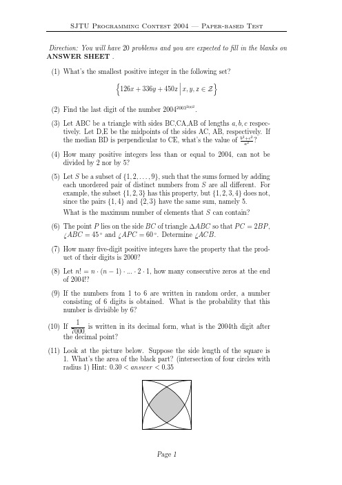
Direction:You will have20problems and you are expected tofill in the blanks on ANSWER SHEET.(1)What’s the smallest positive integer in the following set?126x+336y+450zx,y,z∈Z(2)Find the last digit of the number200420032002.(3)Let ABC be a triangle with sides BC,CA,AB of lengths a,b,c respec-tively.Let D,E be the midpoints of the sides AC,AB,respectively.If the median BD is perpendicular to CE,what’s the value of b2+c2a2? (4)How many positive integers less than or equal to2004,can not bedivided by2nor by5?(5)Let S be a subset of{1,2,...,9},such that the sums formed by addingeach unordered pair of distinct numbers from S are all different.For example,the subset{1,2,3}has this property,but{1,2,3,4}does not, since the pairs{1,4}and{2,3}have the same sum,namely5.What is the maximum number of elements that S can contain?(6)The point P lies on the side BC of triangle∆ABC so that P C=2BP,ABC=45◦and AP C=60◦.Determine ACB.(7)How manyfive-digit positive integers have the property that the prod-uct of their digits is2000?(8)Let n!=n·(n−1)·...·2·1,how many consecutive zeros at the endof2004!?(9)If the numbers from1to6are written in random order,a numberconsisting of6digits is obtained.What is the probability that this number is divisible by6?(10)If17000is written in its decimal form,what is the2004th digit afterthe decimal point?(11)Look at the picture below.Suppose the side length of the square is1.What’s the area of the black part?(intersection of four circles withradius1)Hint:0.30<answer<0.35Page1(12)Five of the six edges of a tetrahedron are known to be at most2004units long.What’s the maximum possible volume of the tetrahedron?(13)Find the smallest positive integer n such that for every integer m with0<m<2004,there exists an integer k for whichm 2004<kn<m+12005.(14)A permutation of the integers1901,1902,···,2003,2004is a sequencea1,a2,···,a104in which each of those integers appears exactly once.Given such a permutation,we form the sequence of partial sumss1=a1,s2=a1+a2,···s104=a1+···+a104 How many of these permutations will have no terms of the sequence s1,···,s104divisible by three?(15)If you know that1+122+132+142+152+···=π26then determine1+132+152+172+192+···(16)How many nonnegative integer solutions for the equationx1+x2+x3+···+x10=2004wherex i≥0and x i∈Z for i=1,2,3,···,10(17)In a box there are four kinds of marbles:20red ones,12yellow ones,8blue ones and6green ones.What is the smallest number of marbles one has to take out of the box to be sure that10marbles are of the same color?(18)Let f(x)=5x13+13x5+9ax.Find the smallest positive integer a suchthat65divides f(x)for every integer x.(19)A small class hasfive students.The teacher collects a test and imme-diately hands it out again such that the students can correct the test themselves.In how many ways can the test be handed out without any student receiving his/her own test?(20)P is a point inside an equilateral triangle such that the distances fromP to the three vertices are3,4and5,respectively.Find the area of the triangle.Page2。

解题报告ACM2004 NERC Gunman【题目描述】三维空间XYZ中,有很多平行于OXY的矩形薄板,并且矩形的边也分别平行于OX,OY。
这些矩形的Z坐标都大于0并且互不相同。
现在有个枪手站在OX轴上,可以任选一个位置向某个方向开1枪。
枪弹的轨迹是直线,并且能够贯穿任意多的矩形。
算出枪手站的位置和开枪的方向,使他能打到所有的矩形。
【分析】不难证明,射出的那条直线,肯定可以通过拉扯和平移,卡在某个矩形的左边界或右边界,同时卡在某个矩形的上边界或者下边界。
那么只需要枚举这两个矩形和分别的边界,再判断,就能在O(N3)的时间复杂度内出解。
这也符合了题目N=100的数据范围。
但是,随着信息学日新月异的发展,O(N3)的算法,已经称不上是高效算法,在竞赛中必然会超时。
下面提出一种时间复杂度O(NLogN)的高效算法。
假设射出的直线的方向是(X,Y,Z),由于把Z除掉,变成(X,Y)。
再设人物的起始点是S。
那么,不难发现,对于任何一个矩形(Z,X min,X max,Y min,Y max),有Y min<=Y*Z<=Y max,即Y min/Z<=Y<=Y max/Z。
将所有的[Y min/Z,Y max/Z]算出来,如果交集为空,那么肯定不能把所有的矩形都射穿。
否则,题目就与Y完全没有关系了,在所有的[Y min/Z,Y max/Z]的交集中任选一个点作为Y,都能满足Y方向上的限制。
现在只考虑X。
对于所有的矩形,都有X min<=X*Z+S<=X max。
这个式子里面有2个未知数,X和S,变下形就是Z*X+S-X min>=0和Z*X+S-X max<=0,可以看成是二维平面X-S中的两个半平面。
在所有的2N个这样的半平面的交集中任取一个点(X,S),都能满足题目的X方向限制。
因此题目成功的转化成求半平面的交的问题了。
而求半平面的交已知是可以做到O(NLogN)的,因此整个算法的时间复杂度就是O(NLogN),比起O(N3)快了巨多。
8期杨一鸣等t时问序列分类问题的算{击比较1265在今后的工作中,我们将会把具体的分类算法[II]考虑进去来做进一步的预处理,考虑怎样的属性组合可以更好地提高我们算法分类的性能.我们也计划把算法运用到其他的多维序列数据集中.参考文献口]Itaku珀EM川mumpre山ctlonr姻ldualpnnclpleappIled8peech舢gnIlIon.IEEET埘mctIonsAcoustlcsSp∞chSlgn且1ProcesB(ASSP).1975t23(1)I52—72[2]Kruska¨JB,LIberIlI皿M.TheBymmetnctImewarm“gal—gonthm,Fromcontl删oustod15crete//T吼eWarps,St“ngEdit8andMacromolecul凹.Addl∞n,1983[3]M”rBc.Rabln盯L,Rosenebe79A.Pcdotradeoffs.ndynaIⅡicn㈣rPmgalgorithmsfor1solatedwordrecog—m“0tI.IEEETfan5actIonsonA洲t瑚SpeechSIgnalProce3s(ASSP)。
1980.28(6):623—635[4]&rⅡdtD,alffordJ.usl“gdynamlctl眦wafplIlgt。
hndpattⅢmt雌鲫es//ProceedlElgso“hAAAI·94work—shopKnowledgenscoveryDataba8e8.s曲ttle,wAtUSA.1994:229—248[5]AachJ,chufchG.A119n1“ggenecxp心5slontImc8盯le8Wltht帅e珊rpillgdgonthm8.Blmnf蝴tl∞,2001.17:495—508[6]白laIIiEG,P。
naAtB聃eIhG,T咖lM,Muzzupappas.Plcruz西F。
-----------------------------最优化问题------------------------------------- ----------------------常规动态规划SOJ1162 I-KeyboardSOJ1685 ChopsticksSOJ1679 GangstersSOJ2096 Maximum SubmatrixSOJ2111 littleken bgSOJ2142 Cow ExhibitionSOJ2505 The County FairSOJ2818 QQ音速SOJ2469 Exploring PyramidsSOJ1833 Base NumbersSOJ2009 Zeros and OnesSOJ2032 The Lost HouseSOJ2113 数字游戏SOJ2289 A decorative fenceSOJ2494 ApplelandSOJ2440 The days in fzkSOJ2494 ApplelandSOJ2515 Ski LiftSOJ2718 BookshelfSOJ2722 Treats for the CowsSOJ2726 Deck of CardsSOJ2729 Space ElevatorSOJ2730 Lazy CowsSOJ2713 Cut the SequenceSOJ2768 BombSOJ2779 Find the max (I) (最大M子段和问题)SOJ2796 Letter DeletionSOJ2800 三角形SOJ2804 Longest Ordered Subsequence (II)SOJ2848 River Hopscotch(二分)SOJ2849 Cow Roller CoasterSOJ2886 Cow WalkSOJ2896 AlphacodeSOJ2939 bailey's troubleSOJ2994 RSISOJ3037 Painting the ballsSOJ3072 ComputersSOJ3078 windy's "K-Monotonic"SOJ3084 windy's cake IVSOJ3104 Game(注意大数运算,高精度)SOJ3110 k Cover of LineSOJ3111 k Median of LineSOJ3123 Telephone WireSOJ3142 Unfriendly Multi Permutation SOJ3213 PebblesSOJ3219 Cover UpSOJ3263 FunctionSOJ3264 Evil GameSOJ3339 graze2SOJ3341 SkiSOJ3352 The Baric BovineSOJ3503 Banana BoxesSOJ3633 Matches's GameSOJ3636 理想的正方形SOJ3711 Mountain RoadSOJ3723 Robotic Invasionnankai1134 Relation Orderingsrm150--div1--500----------------背包问题SOJ2222 Health PowerSOJ2749 The Fewest CoinsSOJ2785 Binary PartitionsSOJ2930 积木城堡SOJ3172 FishermanSOJ3300 Stockholm CoinsSOJ3360 Buying HaySOJ3531 Number Pyramids----------------状态DPSOJ2089 lykooSOJ2768 BombSOJ2819 AderSOJ2842 The TSP problemSOJ3025 Artillery(状态DP)SOJ3088 windy's cake VIIISOJ3183 Fgjlwj's boxesSOJ3259 Counting numbersSOJ3262 Square Fields(二分+状态DP) SOJ3371 Mixed Up CowsSOJ3631 Shopping Offers----------------树状DPSOJ 1870 Rebuilding RoadsSOJ 2136 Apple(树形依赖背包n*C算法)SOJ 2514 Milk Team SelectSOJ 2199 Apple TreeSOJ 3295 Treeland ExhibitionSOJ 3635 World Cup 2010hdoj1561 The more, The BetterPKU1655 Balancing ActPKU3107 GodfatherPKU3345 Bribing FIPAPKU2378 Tree CuttingPKU3140 Contestants DivisionPKU3659 Cell Phone Network---------------配合数据结构的优化DPSOJ 2702 AlannaSOJ 2978 TasksSOJ 3234 Finding SeatsSOJ 3540 股票交易-------------- 斜率优化SOJ 3710 特别行动队SOJ 3734 搬家SOJ 3736 Lawrence of Arabia---------------四边形不等式SOJ 1702 Cutting SticksSOJ 2775 Breaking Strings--------------- 最优化之排序(思考两个元素之间的先后关系,以此得出一个二元比较关系,并验证此关系可传递,反对称,进而排序)SOJ2509 The Milk QueueSOJ2547 cardsSOJ2850 Protecting the FlowersSOJ2957 Setting ProblemsSOJ3167 ComputerSOJ3331 Cards(2547加强版)SOJ3327 Dahema's Computer(通过此题学会排序)-----------------最优化之必要条件枚举(思考最优解所具有的性质,得出最优解的一个强必要条件,在此基础上枚举)SOJ3317 FGJ's PlaneSOJ3429 Food portion sizes--------------------------------贪心---------------------------------------SOJ1078 BlueEyes' ScheduleSOJ1203 Pass-MurailleSOJ1673 Gone FishingSOJ2574 pieSOJ2645 Buy One Get One FreeSOJ2701 In a CycleSOJ2876 Antimonotonicity(经典模型 O(n)算法)SOJ3343 Tower--------------------------------搜索--------------------------------------- SOJ1106 DWeepSOJ1626 squareSOJ2061 8 puzzleSOJ2485 SudokuSOJ1045 SticksSOJ2736 FliptileSOJ2771 Collecting StonesSOJ2715 Maze BreakSOJ2518 Magic Cow ShoesSOJ2829 binary strings(双向BFS)SOJ3005 Dropping the stonesSOJ3136 scu07t01的迷宫(BFS预处理然后枚举交汇点)SOJ3330 Windy's Matrix(BFS)--------------------------------DFA---------------------------------------- ---------------状态矩阵SOJ1826 Number SequenceSOJ1936 FirepersonsSOJ2552 Number of TilingsSOJ2919 Matrix Power Series (学习矩阵的快速乘法从此开始)SOJ2920 Magic BeanSOJ3021 Quad TilingSOJ3046 Odd Loving BakersSOJ3176 E-stringSOJ3246 Tiling a Grid With DominoesSOJ3323 K-Satisfied NumbersSOJ3337 Wqb's Word----------------DFA+DPSOJ1112 Repeatless Numbers(DFA+二分)SOJ2913 Number SubstringSOJ2826 Apocalypse SomedaySOJ3128 windy和水星 -- 水星数学家 1SOJ3182 Windy numbers---------------------------------图论-----------------------------------------------------------最短路SOJ1697 Cashier EmploymentSOJ2325 Word TransformationSOJ2427 Daizi's path systemSOJ2468 CatcusSOJ2751 Wormholes(SPFA判断负圈回路的存在性)SOJ2932 道路SOJ3160 Clear And Present DangerSOJ3335 Windy's Route(最短路径的分层图思想)SOJ3346 Best Spot(N^3放心的写)SOJ3423 Revamping Trails---------------------查分约束SOJ1687 Intervals---------------------最小生成树SOJ1169 NetworkingSOJ2198 HighwaysSOJ3366 Watering HoleSOJ3427 Dark roads---------------------强连通分支SOJ2832 Mars city---------------------2-SATSOJ3535 Colorful DecorationHDU3062 Party---------------------拓扑排序SOJ1075 BlueEyes and Apples (II)---------------------无向连通图上的割点和割边问题SOJ1935 ElectricityWHU145 Railway---------------------二分图的匹配------------------最大匹配SOJ1183 Girls and BoysSOJ1186 CoursesSOJ2035 The Tiling ProblemSOJ2077 Machine ScheduleSOJ2160 Optimal MilkingSOJ2342 Rectangles(Beloved Sons 模型)SOJ2472 Guardian of DecencySOJ2681 平方数 2SOJ2737 AsteroidsSOJ2764 Link-up GameSOJ2806 LED DisplaySOJ2958 Weird FenceSOJ3043 Minimum CostSOJ3038 Beloved Sons(简单贪心一下)SOJ3453 Stock ChartsZOJ3265 Strange Game---------------最佳匹配SOJ1981 Going HomeWHU1451 Special Fish---------------------最近公共祖先问题SOJ1187 Closest Common AncestorsSOJ1677 How far awaySOJ3023 NetworkSOJ3098 Bond---------------------其他SOJ3013 treeSOJ3056 Average distance(树上的DFS)---------------------------------网络流------------------------------------- ---------------------最大流POJ 1273 Drainage DitchesPOJ 1274 The Perfect Stall (二分图匹配)POJ 1698 Alice's ChancePOJ 1459 Power NetworkPOJ 2112 Optimal Milking (二分)POJ 2455 Secret Milking Machine (二分)POJ 3189 Steady Cow Assignment (枚举)POJ 1637 Sightseeing tour (混合图欧拉回路)POJ 3498 March of the Penguins (枚举汇点)POJ 1087 A Plug for UNIXPOJ 1149 Pigs (构图题)ZOJ 2760 How Many Shortest Path (边不相交最短路的条数)POJ 2391 Ombrophobic Bovines (必须拆点,否则有BUG)WHU 1124 Football Coach (构图题)SGU 326 Perspective (构图题,类似于 WHU 1124)UVa 563 CrimewaveUVa 820 Internet BandwidthPOJ 3281 Dining (构图题)POJ 3436 ACM Computer FactoryPOJ 2289 Jamie's Contact Groups (二分)SGU 438 The Glorious Karlutka River =) (按时间拆点)SGU 242 Student's Morning (输出一组解)SGU 185 Two shortest (Dijkstra 预处理,两次增广,必须用邻接阵实现,否则 MLE) HOJ 2816 Power LinePOJ 2699 The Maximum Number of Strong Kings (枚举+构图)ZOJ 2332 GemsJOJ 2453 Candy (构图题)SOJ 2414 Leapin' LizardsSOJ 2835 Pick Up PointsSOJ 3312 Stockholm KnightsSOJ 3353 Total Flow--------------------最小割SOJ2662 PlaygroundSOJ3106 Dual Core CPUSOJ3109 Space flightSOJ3107 SelectSOJ3185 Black and whiteSOJ3254 Rain and FgjSOJ3134 windy和水星 -- 水星交通HOJ 2634 How to earn moreZOJ 2071 Technology Trader (找割边)HNU 10940 CoconutsZOJ 2532 Internship (找关键割边)POJ 1815 Friendship (字典序最小的点割集)POJ 3204 Ikki's Story I - Road Reconstruction (找关键割边)POJ 3308 ParatroopersPOJ 3084 Panic RoomPOJ 3469 Dual Core CPUZOJ 2587 Unique Attack (最小割的唯一性判定)POJ 2125 Destroying The Graph (找割边)ZOJ 2539 Energy MinimizationZOJ 2930 The Worst ScheduleTJU 2944 Mussy Paper (最大权闭合子图)POJ 1966 Cable TV Network (无向图点连通度)HDU 1565 方格取数(1) (最大点权独立集)HDU 1569 方格取数(2) (最大点权独立集)HDU 3046 Pleasant sheep and big big wolfPOJ 2987 Firing (最大权闭合子图)SPOJ 839 Optimal Marks (将异或操作转化为对每一位求最小割)HOJ 2811 Earthquake Damage (最小点割集)2008 Beijing Regional Contest Problem A Destroying the bus stations ( BFS 预处理 )(http://acmicpc-live-archive.uva.es/nuevoportal/data/problem.php?p=4322)ZOJ 2676 Network Wars (参数搜索)POJ 3155 Hard Life (参数搜索)ZOJ 3241 Being a Hero-----------------有上下界ZOJ 2314 Reactor Cooling (无源汇可行流)POJ 2396 Budget (有源汇可行流)SGU 176 Flow Construction (有源汇最小流)ZOJ 3229 Shoot the Bullet (有源汇最大流)HDU 3157 Crazy Circuits (有源汇最小流)-----------------最小费用流HOJ 2715 Matrix3HOJ 2739 The Chinese Postman ProblemPOJ 2175 Evacuation Plan (消一次负圈)POJ 3422 Kaka's Matrix Travels (与 Matrix3 类似)POJ 2516 Minimum Cost (按物品种类多次建图)POJ 2195 Going HomePOJ 3762 The Bonus Salary!BUAA 1032 Destroying a PaintingPOJ 2400 Supervisor, Supervisee (输出所有最小权匹配)POJ 3680 IntervalsHOJ 2543 Stone IVPOJ 2135 Farm TourSOJ 3186 SegmentsSOJ 2927 终极情报网SOJ 3634 星际竞速HDU 3376 Matrix Again-----------------------------------数据结构--------------------------------- -----------------------------------基础数据结构----------------------栈SOJ2511 MooooSOJ3085 windy's cake V(经典栈与单调性的结合)SOJ3279 hm 与 zx 的故事系列2SOJ3329 Maximum Submatrix II(转化为上面两题的模型)---------------------双端队列SOJ2978 TasksSOJ3139 Sliding Window(双端队列最经典的应用)SOJ3636 理想的正方形-------------------- --------------高级数据结构---------------------线段树SOJ1862 Choice PearsSOJ2057 The manager's worrySOJ2249 Mayor's postersSOJ2309 In the Army NowSOJ2436 Picture puzzle gameSOJ2556 Find the PermutationSOJ2562 The End of CorruptionSOJ2719 Corral the Cows(线段树+二分)SOJ2740 Balanced LineupSOJ2745 零序列SOJ2776 Matrix SearchingSOJ2808 Thermal Death of the UniverseSOJ2822 Buy TicketsSOJ2937 TetrisSOJ2938 Apple Tree(先DFS获得欧拉序列)SOJ2965 capitally playersSOJ2968 Matrix(二维线段树)SOJ3019 Count ColorSOJ3022 Difference Is Beautiful( RMQ+二分经典模型)SOJ3086 windy's cake VI(二维线段树)SOJ3099 A Simple Problem with IntegersSOJ3248 MousetrapSOJ3321 Windy's Sequence IISOJ3370 Light SwitchingSOJ3640 Special Subsequence---------------------树状数组SOJ2309 In the Army Now---------------------归并排序思想SOJ2906 Ultra-QuickSortSOJ2431 Cows distribute food(利用归并排序求逆序数:nlogn) SOJ2497 Number sequenceSOJ2559 What is the Rank?SOJ2728 MooFestSOJ3009 Stones for AmySOJ3010 K-th NumberSOJ3147 K-th number---------------------并查集SOJ1824 The SuspectsSOJ1953 keySOJ2245 Ubiquitous ReligionsSOJ2389 Journey to TibetSOJ2438 PetSOJ2490 Math teacher's testPOJ2832 How many pairs?POJ2821 Auto-Calculation MachineSOJ2979 食物链SOJ3282 Kingdom of HeavenSOJ3417 Skyscrapers------------------------块状链表SOJ3032 Big StringSOJ3035 反转序列----------------------------------- 字符串---------------------后缀数组SOJ1948 sekretarkaSOJ3045 Long Long MessageSOJ3075 回文子串SOJ3296 Windy's S---------------------KMPSOJ2652 OulipoSOJ2307 String MatchingSOJ3014 Seek the Name, Seek the FameSOJ3596 Article Decryption--------------------trie树SOJ3076 相同字符串SOJ3336 DiarySOJ3596 Article Decryption---------------------------------组合数学及数论----------------------------- SOJ1839 Relatives(Euler函数)SOJ1942 FotoSOJ2714 Mountains (II)SOJ2668 C(n,k)SOJ2666 分解 n!SOJ2106 GCD & LCM InverseSOJ2498 Count primeSOJ2238 Let it Bead(置换群-polya定理的应用)SOJ2924 完美交换(置换群)SOJ2638 Cow Sorting(置换群)-------------费马小定理SOJ 3578 H1N1's Problem--------------------------容斥原理SOJ3191 Free squareSOJ3082 windy's cake IISOJ3502 The Almost Lucky NumbersSOJ3547 Coprime----------------------------------博弈论------------------------------------SOJ1128 控制棋SOJ1866 Games(诡异的博弈)SOJ2197 A Funny GameSOJ2188 A multiplication gameSOJ2403 Black and white chessSOJ2477 Simple GameSOJ2687 草稿纸 2SOJ2688 草稿纸 3SOJ2836 Pick Up Points IISOJ2845 JangeSOJ2922 A New Tetris GameSOJ2993 NimSOJ3066 JohnSOJ3132 windy和水星 -- 水星游戏 1SOJ3133 windy和水星 -- 水星游戏 2SOJ3174 Good gameSOJ3307 Stockholm GameSOJ3446 Nim or not NimSOJ3461 Nim-kSOJ3463 Ordered NimSOJ3468 Flip CoinsSOJ3548 gameSOJ3584 Baihacker and Oml-----------------------------------计算几何---------------------------------SOJ1138 WallSOJ1102 Picnic。