元胞自动机交通流模型 PPT

融合多源信息的元胞自动机交通流模型随着城市化进程的不断发展和交通流量的快速增长，如何合理优化城市交通系统成为了亟待解决的问题。

为了解决交通流量管理中遇到的挑战，研究人员开始使用元胞自动机交通流模型作为一种有效的工具。

元胞自动机交通流模型结合了多源信息，并能够对城市道路网络中的交通流进行模拟和预测。

本文将重点介绍融合多源信息的元胞自动机交通流模型，并详细分析其优势和应用前景。

一、元胞自动机交通流模型简介元胞自动机交通流模型是一种基于交通流动的个体自动行为的模拟方法。

它将整个道路网络划分为多个元胞，每个元胞代表一个交通单元，如车辆或行人等。

通过定义元胞之间的规则和交互方式，模型可以刻画城市道路系统中的交通流动情况。

元胞自动机交通流模型使用自动机理论和网络拓扑结构相结合的方法，具有模拟真实交通行为的优势。

二、多源信息融合的意义和方法多源信息的融合对于提高交通流模型的准确度和预测能力至关重要。

常见的多源信息包括道路网络拓扑结构、车辆速度、交通信号灯状态、道路岔口等。

通过合理融合这些信息，可以更好地模拟城市交通流动的实际情况。

在元胞自动机交通流模型中，多源信息融合的方法主要包括以下几种：数据融合、模型融合和参数融合。

数据融合是将来自不同数据源的交通数据进行处理和整合，以获取全面准确的信息。

模型融合是将不同类型的交通模型进行整合，并基于多种模型的结果进行预测和优化。

参数融合是将不同参数的评估结果进行整合，以获取更加全面和准确的评估结果。

三、融合多源信息的元胞自动机交通流模型的优势融合多源信息的元胞自动机交通流模型相比传统模型具有以下优势：1. 准确性提高：多源信息的融合使得模型更加贴近真实交通情况，模拟结果更准确可靠。

2. 鲁棒性增强：多源信息的融合使得模型对于数据噪声和不确定性具有更好的适应和鲁棒性。

3. 预测能力增强：多源信息的融合使得模型在预测和优化交通流方面具有更高的准确性和可信度。

四、融合多源信息的元胞自动机交通流模型的应用前景融合多源信息的元胞自动机交通流模型在城市交通系统优化和管理中具有广阔的应用前景。

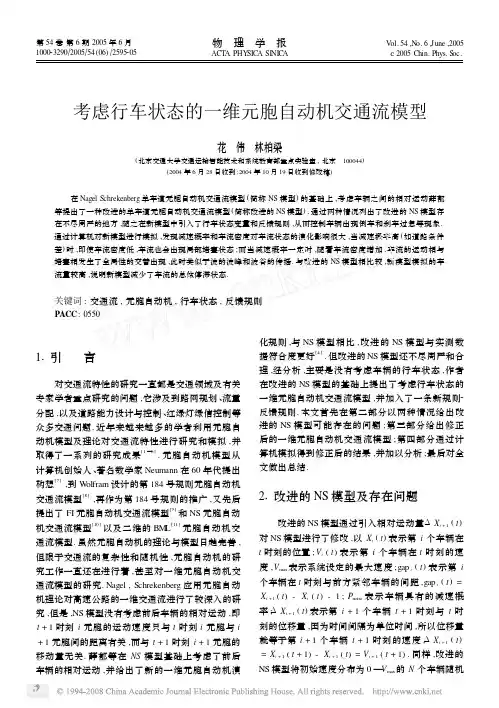
考虑行车状态的一维元胞自动机交通流模型花　伟　林柏梁(北京交通大学交通运输智能技术和系统教育部重点实验室,北京　100044)(2004年6月28日收到;2004年10月19日收到修改稿) 在Nagel Schrekenberg单车道元胞自动机交通流模型(简称NS模型)的基础上,考虑车辆之间的相对运动薛郁等提出了一种改进的单车道元胞自动机交通流模型(简称改进的NS模型).通过两种情况列出了改进的NS模型存在不尽周严的地方,随之在新模型中引入了行车状态变量和反馈规则,从而控制车辆出现倒车和刹车过急等现象.通过计算机对新模型进行模拟,发现减速概率和车流密度对车流状态的演化影响很大,当减速概率高(如道路条件差)时,即使车流密度低,车流也会出现局部堵塞状态;而当减速概率一定时,随着车流密度增加,车流的运动相与堵塞相发生了全局性的交替出现,此时类似于波的波峰和波谷的传播.与改进的NS模型相比较,新模型模拟的车流量较高,说明新模型减少了车流的总体停滞状态.关键词:交通流,元胞自动机,行车状态,反馈规则PACC:055011引言对交通流特性的研究一直都是交通领域及有关专家学者重点研究的问题,它涉及到路网规划、流量分配,以及道路能力设计与控制、红绿灯绿信控制等众多交通问题.近年来越来越多的学者利用元胞自动机模型及理论对交通流特性进行研究和模拟,并取得了一系列的研究成果[1—6].元胞自动机模型从计算机创始人、著名数学家Neumann在60年代提出构想[7],到W olfram设计的第184号规则元胞自动机交通流模型[8],再作为第184号规则的推广,又先后提出了FI元胞自动机交通流模型[9]和NS元胞自动机交通流模型[10]以及二维的BM L[11]元胞自动机交通流模型.虽然元胞自动机的理论与模型日趋完善,但限于交通流的复杂性和随机性,元胞自动机的研究工作一直还在进行着,甚至对一维元胞自动机交通流模型的研究.Nagel,Schrekenberg应用元胞自动机理论对高速公路的一维交通流进行了较深入的研究,但是,NS模型没有考虑前后车辆的相对运动,即t+1时刻i元胞的运动速度只与t时刻i元胞与i +1元胞间的距离有关,而与t+1时刻i+1元胞的移动量无关.薛郁等在NS模型基础上考虑了前后车辆的相对运动,并给出了新的一维元胞自动机演化规则,与NS模型相比,改进的NS模型与实测数据符合度更好[4].但改进的NS模型还不尽周严和合理,经分析,主要是没有考虑车辆的行车状态,作者在改进的NS模型的基础上提出了考虑行车状态的一维元胞自动机交通流模型,并加入了一条新规则2反馈规则.本文首先在第二部分以两种情况给出改进的NS模型可能存在的问题;第三部分给出修正后的一维元胞自动机交通流模型;第四部分通过计算机模拟得到修正后的结果,并加以分析;最后对全文做出总结.21改进的NS模型及存在问题改进的NS模型通过引入相对运动量ΔXi+1(t)对NS模型进行了修改,以Xi(t)表示第i个车辆在t时刻的位置;V i(t)表示第i个车辆在t时刻的速度,Vmax表示系统设定的最大速度;gapi(t)表示第i个车辆在t时刻与前方紧邻车辆的间距,gapi(t)= X i+1(t)-X i(t)-1;P noise表示车辆具有的减速概率;ΔXi+1(t)表示第i+1个车辆t+1时刻与t时刻的位移量,因为时间间隔为单位时间,所以位移量就等于第i+1个车辆t+1时刻的速度,ΔXi+1(t) =X i+1(t+1)-X i+1(t)=V i+1(t+1).同样,改进的NS模型将初始速度分布为0—V max的N个车辆随机第54卷第6期2005年6月100023290Π2005Π54(06)Π2595205物　理　学　报ACT A PHY SIC A SI NIC AV ol.54,N o.6,June,2005ν2005Chin.Phys.S oc.地分布在长度为L 的一维离散的格点链上,并在考虑周期边界条件下,给出间距的确定规则如下:(1)确定所有车辆i 在t +1时刻的速度分布:IF (V i (t )≥gap i (t )+ΔX i +1(t )):V i (t +1)=gap i (t )+ΔX i +1(t )-1,以概率p noise gap i (t )+ΔX i +1(t ),其他　(跟车Π减速规则),E LSE IF (V i (t )<V max )V i (t +1)=V i (t ),以概率p noise V i (t )+1,其他　(加速规则),E LSE IF (V i (t )=V max 且V i (t )<gap i (t )+ΔX i +1(t ))V i (t +1)=V max -1,以概率p noise V max ,其他　(自由运动规则). (2)确定所有车辆i 在t +1时刻的位置:X i (t +1)=X i (t )+V i (t +1) 下面用两种情况指出改进的NS 模型中可能存在的问题:情况1　在t 时刻,如果V i +1(t )=0,V i (t )=0,gap i (t )=0,那么在t +1时刻,当V i +1(t +1)=0,则ΔX i +1(t )=0(),车辆i 满足条件V i (t )≥gap i (t )+ΔX i +1(t ),则按跟车Π减速规则,得到V i (t +1)=-1,以概率p noise ,0,其他. 如何解释V i (t +1)以概率P noise 等于-1?再者,理论上V i (t +1)必定等于0,而不是以某一概率等于0.情况2　在t 时刻,如果V i +1(t )=1,V i (t )=4,gap i (t )=4,那么在t +1时刻,当V i +1(t +1)=0,则ΔX i +1(t )=0(停车状态),车辆i 满足条件V i (t )≥gap i (t )+ΔX i +1(t ),则按跟车Π减速规则,得到V i (t +1)=3,　以概率p noise ,4,　其他,gap i (t +1)=1,　当V i (t +1)=3,0,　当V i (t +1)=4. 这里可以看到,当前车停车后,后车速度比较快时,后车仍以1-P noise 的概率跟车,而没有采取减速措施,虽然模型中的后车不会碰上前车,但这是不符合车流特性的.再推进一个时间步,即t +2时刻,取V i (t +1)=4(跟车),当V i +1(t +2)=0,则ΔX i +1(t +1)=0(停车状态),车辆i 满足条件V i (t +1)≥gap i (t +1)+ΔX i +1(t +1),则按跟车Π减速规则,得到V i (t +2)=-1,以概率p noise ,0,其他. 这里仍存在V i (t +2)=-1,即倒车现象.另外可以看出,前车在刹车两个时间步后,后车是一步刹车而减为0,如果在满足刹车条件时先减速,再刹车可能更符合车流特性.从情况1和情况2可以看出,改进的NS 模型虽然将车辆间的相对运动量引入了NS 模型,但没有将前车的行车状态考虑进模型中,所以出现倒车、刹车过急等不尽周严和合理的现象.31考虑前车行车状态的新模型新的模型将前车的行车状态分成停车状态和行进状态,用δi +1(t )表示前车t 时刻的行车状态:δi +1(t )=1,　当ΔX i +1(t )=0(停车状态),0,　当ΔX i +1(t )>0(行进状态),其他变量定义同前,在模型中同时还添加了反馈规则,以避免不尽合理的急刹车.在本模型中仍是将初始速度分布为0—V max 的N 个车辆随机地分布在长度为L 的一维离散的格点链上,在考虑周期边界条件下,给出间距的确定规则如下:1)确定所有车辆i 在t +1时刻的速度分布:6952物 理 学 报54卷IF (V i (t )≥gap i (t )+ΔX i +1(t )):(减速规则)　V i (t +1)=0,当gap i (t )=0(后车必停车)gap i (t )-1,当gap i (t )>0(后车必减速),当δi +1(t )=1　V i (t +1)=gap i (t )+ΔX i +1(t )-1,以概率p noise gap i (t )+ΔX i +1(t ),以概率1-p noise,当δi +1(t )=0E LSE 2IF (V i (t )<V max ):(加速规则)　V i (t +1)=V i (t ),以概率p noiseV i (t )+1,以概率1-p noise E LSE (V i (t )=V max ):(自由运动规则)　V i (t +1)=V max -1,以概率p noise V max ,以概率1-p noiseIF (V i (t +1)=gap i (t )且gap i (t )>1):V i (t +1)=V i (t +1)-δi +1(t )(反馈规则) 2)确定所有车辆i 在t +1时刻的位置:X i (t +1)=X i (t )+V i (t +1). 根据上述规则进行模拟,并由一维格点链计算公式:车辆密度ρ=N L,t 时刻的平均速度 V (t )=1N∑Ni =1V i (t ),及t 时刻的平均车流量 J (t )=ρ× V (t ),ρ2V 关系曲线、车流量与车辆密度的ρ2J 关系曲线,以及平均速度与车流量V 2J 关系曲线.其中N 为分布在格点链L 上的车辆数.模拟中的道路长度L 为715km ,用1000个格点表示,车辆以初始速度分布为0—V max 随机地分布在1000个一维离散的格点上,边界为周期边界条件.如果取单位时间步长为1s ,则最大速度V max =5相当于135km Πh.因为模拟中采取了周期边界条件,所以对于某次模拟,格点中的车辆数N 固定不变,那么车流密度ρ也是常数.因此,通过改变每次模拟中的车流密度和减速概率P noise ,可以观察对应车流速度和车流量的变化趋势.41计算机模拟及分析通过计算机模拟结果可知,减速概率P noise 对车流速度的影响相当大,在文献[4]中作者给出了减速概率与车辆密度的关系,但减速概率还同路况、驾驶员等诸多因素有关,所以本文中没有沿用文献[4]中的关系式,而取P noise 为0110,0125和0150三种概率进行模拟比较;每次模拟的总时间步长为60000个单位时间步,所有的平均速度为50000—55000时间步内的算术平均值,这样可以避免初始状态的影响;每个时间步车辆i 选择规则所需的随机数满足0—1平均分布,且相互独立.图1所示为车辆位置随时间推移的演化过程图,取400格点后的车流位置:(a )部分为车辆密度ρ=0109、减速概率P noise =0109条件下的车流演化过程.可以看出整个车流位置呈线形演化,基本维持车辆间距不变;(b )部分为车辆密度ρ=0109、减速概率P noise =0180条件下的车流演化过程.虽然车流密度很低,但在局部地方还是发生了车辆较长时间的停滞,并引起后续车辆的停滞.由此可以看出:减速概率对车流行进的影响很大,而且车辆一旦停滞,由于减速概率大,加速概率小,所以车流启动也很缓慢;(c )部分为车辆密度ρ=0150、减速概率P noise =0150条件下的车流演化过程.图示中存在很明显的“波”传递过程,竖黑线部分表示车辆停滞状态,白色断层部分表示车辆行进状态,由于车辆密度高,减速概率大,所以前车的行车状态对后续车辆的行车状态影响很大.图2给出了不同减速概率下的车流密度ρ与平均速度V 的关系图.同样看出减速概率对车流速度的影响很明显,近线性关系;在车流密度较小时,车流速度变化不大;当车流密度达到一定程度时,车流速度出现了明显的拐点;车流速度为零,即发生大面积堵塞时,车流密度还没有达到0190,从理论上分析,只要密度不等于1100,车辆间就有空格,那么个别车辆会爬行,出现这种结果与计算机的计算精度有关.图2中,对应P noise =0110的ρ2V 曲线:最大的平均速度V =132132km ・h-1;当ρ=0146时,车速出现拐点,此时平均速度V =130154km ・h-1;当平均速79526期花　伟等:考虑行车状态的一维元胞自动机交通流模型度V 接近零时,ρ=0176.对应P noise =0125的ρ2V 曲线:最大的平均速度V =128191km ・h -1;当ρ=0123时,车速出现拐点,此时平均速度V =123160km ・h -1;当平均速度V 接近零时,ρ=0162.对应P noise =0150的ρ2V 曲线:最大的平均速度V =121165km ・h-1;当ρ=0111时,车速出现拐点,此时平均速度V=119100km ・h -1;当平均速度V 接近零时,ρ=0156.从模拟结果看,无论密度多小,减速概率多小,车速都没有达到最大速度135100km ・h -1,这说明车辆速度存在波动.图1　位置与时间关系图图2　对应不同P n oise 的平均速度V 与密度ρ关系图图3　对应不同P n oise 的平均速度V 与流量J 关系图 图3给出了不同减速概率下的平均速度V 与流量J 的关系图.当在一定车速范围内,车流量呈线性增加,但车速到达某一速度值后,车流量反呈非线性递减;当车速太快(密度小)和太慢时,流量都很小.对应P noise =0110的V 2J 曲线:当车速最大,即V =132120km ・h -1时,流量J =88113veh ・h -1;当车速在132120—130171km ・h -1时,流量呈线性递增;当车速V =130100km ・h -1时,流量出现拐点,即达到最大值,J max =6760100veh ・h -1;当车速在130100—0100km ・h -1时,流量呈非线性递减.对应P noise =0125的V 2J 曲线:当车速最大,即V =128141km ・h -1时,流量J =85160veh ・h -1;当车速在128141—125160km ・h -1时,流量呈线性递增;当车速V =123134km ・h -1时,流量出现拐点,即达到最大值,J max =3617197veh ・h -1;当车速在123134—0100km ・h -1时,流量呈非线性递减.对应P noise =0150的V 2J 曲线:当车速最大,即V =121152km ・h -1时,流量J =81103veh ・h -1;当车速在121152—120152km ・h -1时,流量呈线性递增;当车速V =119100km ・h -1时,流量出现拐点,即达到最大值,J max =1904100veh ・h -1;当车速在119100—0100km ・h -1时,流量呈非线性递减.与NS 模型和改进的NS 模型相比较,车流量总体偏大,说明车流总体停滞次数减少.51结　论本文通过两种情况指出改进的NS 模型存在着8952物 理 学 报54卷不尽周严的问题,随之引入行车状态变量,在前车停止行进时,后车相应采取减速措施,而不是随机减速;另外,补充了一条全新的车辆运动规则———反馈规则,进一步控制车辆的急刹车现象.计算机模拟结果显示,车流量相比增大,这是车流总体停滞次数减少的结果,说明改进模型是有效的.[1]W ang B H et al 1998Acta Phys .Sin .47906(in Chinese )[汪秉宏等1998物理学报47906][2]L üX Y et al 1998Acta Phys .Sin .471761(in Chinese )[吕晓阳等1998物理学报471761][3]Huang P H et al 2001Acta Phys .Sin .5030(in Chinese )[黄乒花等2001物理学报5030][4]Xue Y et al 2001Acta Phys .Sin .50445(in Chinese )[薛　郁等2001物理学报50445][5]T an H L et al 2002Acta Phys .Sin .512713(in Chinese )[谭惠丽等2002物理学报512713][6]Xue Y 2004Acta Phys .Sin .5325(in Chinese )[薛　郁2004物理学报5325][7]Neumann V 1966Theory o f Self 2Reproducing Automata (Urbana :University of Illinois Press )[8]W olfram S 1986Theory and Application o f Cellular Automata (S ingapore :W orld Scientific )[9]Ishibashi Y and Fukui M 1994J .Phys .Soc .Japan ,632882[10]Nagel K and Schrekenberg M 1992J .Physique I France 22221[11]Biham O ,M iddleton A A and Levine D 1992Phys .Rev .A 46R6124One -dimensional traffic cellular automaton modelwith considering the vehicle moving statusHua W ei Lin Bo-Liang(K ey Laboratory o f Intelligent Technologies and Systems o f Tra ffic and Transportation ,Beijing Jiaotong Univer sity ,Beijing 100044,China )(Received 28June 2004;revised manuscript received 19October 2004)AbstractBased on the single lane traffic cellular automaton (C A )m odel introduced by Nagel and Schreckenberg (called NS m odel ),Xue Y u et al proposed an im proved single lane traffic C A m odel by considering the relative m otion of vehicles (called im proved NS m odel ).Several faults in the im proved NS m odel using tw o exam ples is pointed out and also another single lane traffic C A m odel by introducing vehicle-m oving -status variable and feedback rule is proposed.These methods help to prevent vehicle from m oving backward and stopping hurry.Numerical simulations are carried out and the results indicate that the deceleration probability and traffic density have a heavy im pact on the ev olution process of traffic flow.Under the condition of high deceleration probability ,there may happen local traffic jams even with low traffic density.And with a constant deceleration probability ,the global free phases and jam phases will appear alternately as the traffic density increases to a certain level.The phenomenon is very sim ilar to the propagation of wave.The traffic flow is higher in the new m odel than in the im proved NS m odel.This proves that the stop status of the whole traffic flow has been im proved.K eyw ords :traffic flow ,cellular automata ,vehicle m oving status ,feedback rule PACC :055099526期花　伟等:考虑行车状态的一维元胞自动机交通流模型。

Research on Traffic Flow Modeling and Simulation Based onCellular AutomatonAbstract:Intelligent transportation system(ITS) improves the situation of transportation systems by managing advanced technologies such as telecommunication, network, automatic control and traffic engineering to, thus establishing an intelligent, secure, convenient, efficient, comfortable and environmental protection transportation system. Traffic flow modeling is one of the most important parts of ITS. ITS can be categorized as microscopic modeling and macroscopic modeling. Microscopic traffic models such as cellular automaton (CA) models and hybrid traffic models arisen in recent years have optential values in application.Key word: CA Traffic flow modelling BicycleI Introduction of Cellular AutomatonThe conception of cellular automaton(CA) was firstly put forward by V on Nenmann in the 1950s, it was mainly applied in modelling the function of self-duplication of biosystem. It was paid widely attention to after the confliction of life was put forward by Conway in 1970. After that, CA was applied to various field. Because a simple model type like this could duplicate complex phenomena or dynamically demonstratephenomena of attraction, self organization and chaos conveniently.That’s the reason why CA was widely used in modeling diverse physical systems and natural phenomena, such as fluld flow, galaxy formation, snowslide, traffic flow calculation, concurrent computation , earthquake etc. Nowadays, the merits of making use of CA to modeling the physical process is that it can leave out the process using differential equations as transition, and performing nolinear physical phenomenon directly through making rules. In these practical applications, CA model uncovers macroscopic behavior naturally happened through simple microscopic partial rules. It’s an ideal physical model for studying temporal-spatial discrete, and considered the most effective implement in terms of researching complex system.CA model is made up of 4 parts basically: cell, lattice, neighbor and rule.Its ordinary features are summarized as follows:Temporal discrete isometry, it means the deduction of system is proceeding according to a uniformly-spaced discrete time distribution, the time step dt usually sets time unit 1.Spatial discrete homogeneity, it reflects that variations of each cell obey the same rule, and the way of distribution of each cell is identical.Status discrete finite, it means the status of CA can only be taken finite discrete values.Calculation synchronously and concurrently. Considering theforming and variation of CA as calculating or disposing of data or information, it will show up that disposing process of CA is synchronous and concurrent, which means it is adapted to concurrent calculation especially.Renew rules partially. The current status of each cell can only be affected by ones of its neighborhood. In terms of information transmission, the velocity of it in CA is finite.Infinite dimension variables. In a dynamic system, the number of variables is often transformed into dimension. Status of each cell is considered as a variable, so a CA model contains infinite cells is regarded as a type of infinite dimension dynamic system.The features above are just some ordinary features of CA models. In practical application, builders of models often extent their CA models more or less, breaking through the limitations above to forming various extended CA models. That’s why the field of CA model application is widely. But every extention to CA should keep its ordinary feature , especially the feature of renew rules partially.In the 1990s, with the demand of traffic flow simulation and the development of intelligent transportation, people attempted to apply the theory of cellular automaton in physics to the field of transportation, so cellular automaton models of traffic flow arised.The merits of traffic flow CA models are: (1) models areuncomplicated, it can be realized on a computer easily. When modeling, divide the road into several cells with a length of L, a cell corresponds to one car or several cars, or several cells correspond to one car. The status of each cell is empty or the velocity of cars that it contains, every car is motivated by a set of rules simultaneously. These rules consist of moving rules and traffic rules that moving vehicle should obey, random rules that contains driving behavior, interference of circumstance. (2)It is capable of recurring various complicated phenomena of transportation, indicating features of traffic flow. In the modeling process, through inspecting the transformation of status of cells, people can acquire the velocity, displacement and headway of every car at any moment which describe microscopic features of traffic flow , with parameters of average velocity, density, flowrate that describe macroscopic features of traffic flow at the same time.1.1 Single Lane CA modelN-S model is a simplified one-dimensional CA model, it was put forward by German bachelors Nagel and Schreckenberg in 1992. it is a minimal one-dimensional CA traffic flow model for describing freeway traffic flow. Each path of it is essential for modeling diverse features practical traffic flow. It provides basic rules for more complicated situation or urban traffic rules.The model use a one-dimensional lattice to indicate a single lane, inother words, divide the researching single lane into n parts (cells) with the length of L. each situation in the lattice corresponds to a cell, and each situation is either empty or containing a car. Defining the length of cell, L as headway when traffic jamming; the velocity of cars range from 0 to vmax, vmax=5 times the length of cell per second; time step can be supposed to the reaction time of drivers, sets 1s in common; there are 7 types of status in each situation, namely empty, the velocity of situation is 0,1,2,3,4 and 5. In the N-S model, the status of all cars are variable simultaneously according to 4 rules listed as follows:Rules of Acceleration : if v(t)≤vmax, then v(t+l)=min(vmax,v(t)+l).Rules of Deceleration : if v(t)>gap, then v(t+1)=gap.Rules of Ramdom : in the probability of P,v(t+1)=max(v(t+1)-1,0).Vehicle Movement: x(t+1)=x(t)+v(t+1).The gap in the rules stands for the empty space between current car and former one. X stands for car’s situation. Because t=1s, vt=v. In this model, Rule of Acceleration reflects that driver accelerates the car to max velocity gradually; Rule of Deceleration reflects driver decelerates the car in order to avoid colliding with former car; Rule of Random indicates the uncertainty of driver’s action. In N-S model, the probability of random deceleration is a critical parameter, when P=0, N-S model is a deterministic traffic CA.From the consequence of modeling, N-S model reflects the macroscopic features of vehicle’s movement well, which represents as follows: (1) it present the phenomenon of start-to-stop waves, which means in a time space diagram, the process that traffic flow varies from free in low density to crowded in high density gradually can be acquired distinctly, indicating a scene that vehicle’s movement is like a wave spreading in the queue vividly. (2) flow-density curve can be obtained from modeling, which is extremely similar with practical consequence, revealing two statuses of traffic flow------ status of crowded and status of uncrowded.N-S Model has two types of boundary condition. One is periodic boundary, the other is the open boundary. Periodic boundary condition is an idealized analysis method of CA model. It means the origination and destination are connected, which is fit for analysis of metastable status when density is stable.Since it takes the form of concurrent update, no exactly analytic solutions can be acquired. But periodic boundary can obtain approximate analytic solutions through simulation, Providing a powerful verification platform for problem analysis. In recent years, this periodic boundary pattern has achieved great success in analysing N-S model and its extentions. The open boundary signifies when a car put in or put off the road, it should accord with certain probability distribution. The open boundary is more fit for practical situation, especially in theaspect of freeway ramp control where traffic engineers concern.N-S model is the simplist type of one-dimensional CA model of traffic flow, 4 rules only turn out the most foundamental characteristic of traffic flow. On the basis of it, people do more kinds of improvement and revision, expect they can reflect the characteristics of traffic flow more accurately.1.2 multiple lanes CA modelThe main measurement to expand a single lane model to a multiple lane model is to set up traffic lane changing rules, many scholars have made contributions in this aspect. Among them, because of the different situation of lanes, such as the difference between fast and slow lane, the double driveway model is divided into symmetric lane model and asymmetric lane model. In addition, depending on the difference of the vehicle, such as there are two or more different maximum speed vehicles, can also be divided into two kinds of model, symmetric and asymmetric. Generally, the update steps of double driveway model are divided into two steps: first step, according to the rules of lane changing changes lanes synchronously; The second step, using single lane model update vehicle location simultaneously. Drivers have two main lane changing demand motivation: one is another lane can drive cars more convenient and gain greater speed; Second is where the vehicle is drivingto a turnning demanding corner, producing motivation of lane changing, and satisfying the safety conditions at the same time. In 1996, Rickert proposed vehicles are allowed to change the way if they fulfill follwing 4 rules:(1)gap(i)<l,(2)gap0(i)>l0,(3)gap0,back(i) l0,back,(4)rand()<Pc,Among them, the gap (i) and gap0(i) correspond to the shorter distance of the vehicle(i) in the current lane to former one in another lane or the vehicle in front of the driveway l; Gap0,back (i) for the minimal distance between the vehicle i and the latter one in another lane;l,l0,l0,back are all consts represent distance; The rand () is the random number between 0 and 1, the Pc stands for lane changing probability.1.3 network CA modelIn 1992, 0. Biliam, arjun iddleton and D.L evine uses cellular automata to design a simple two-dimensional cellular automata model (BML model) to simulate the urban network traffic flow phenomenon and research the traffic jam problem. Simulation results showed that when the vehicle density was greater than a critical value, the block would happen. BML model is simple and intuitive. In this model, an NxN squarelattice, N is the length of lattice, each lattice can have a north-south traffic, or have a east-west traffic,or nothing. In every odd time step, north-south vehicle can drive forward a lattice; In every even number of time steps, east-west vehicle can go forward a lattice; If just in front of one vehicle ,there’s another vehicle in lattice ,then it have to wait in place, the car can't driving forward. In this way, each lattice point is the equivalent of intersection signal control.However BML model has very big disparity with the actual traffic conditions , mainly displays in:(1) the abstract and simplification of the BML model to the transportation network is unreasonable, it only has intersections in the network diagram, there is no road;(2) the BML model simplifies the traffic movement in two directions, without considering steering movement, leading to large difference with the actual situation.In 1999, Chowdhu cut and Schadschneider put forward a more realistic two-dimensional CA traffic flow model, which is use D cellular stands for each section of the street, the street can utilize Nasch model to stimulate, and distance between two adjacent intersection D-1cell-length, as shown in figure below.At each intersection set red and green Light, when one direction is accessible, another direction is in prohibition, with period T change. Vehicles moving forward until the cell was dominated by other vehicles ahead or meet the crossing when the red light is on. The parallel update rules are as follows:1) acceleration: vn to min(vn +1,vmax);2) deceleration: set dn is the nth Car's front spacing, sn is the distance between it and the location of the traffic lights ahead, Specific points two situations:Lights for the nth car is red vn to min(vn, dn-1 ,sn-1);(2) when the signal for the nth car is green, make the remaining time that light turned red t, there are following three conditions: If dn<Sn ,then vn to min(vn, dn-1);If dn>Sn and min(vn,dn-1)*t>sn, then vn ->min(vn,dn-1);if dn>Sn and min(Vn,dn-1)*t<Sn,then vn to min(vn, sn-1);Namely the speed of the vehicle depends on whether it can throughthe intersection before the red light is on;3) randomization.Vn tends to max(Vn-1,0) in the probability of p;4) location update . east to vehicles: Xn = Xn+.vn; North of the vehicle; Yn = Yn +.vn.At an initialization time, N→and N↑vehicles are randomly placed in the model, according to the rules above for parallel refreshing. From free flow phase to crowding phase ,the transformation point of density c * (D), with the model parameters, it p, vmax, T the relationship among them has not yet fully cleared. From computer simulation data cannot prove that it has nothing to do with these parameters, inducing of blockage of dynamic randomness is consistent with the BML model, the block that self-organization leads to is basically the same with BML model.However, the average speed of the model changes over time, and in the liquid phase as the density. deceleration probability p, road length D, the change of the signal period T is closer to reality than the BML model.The model can also be improved in the following aspects: (l) multiple lanes; (2)set realistic vehicle steering rules at the intersection : (3) set different types of lights, including green wave band.II. Bicycle traffic flow stimulation and application2.1 bicycle traffic flow characteristics and the bicycle characteristicsThe characteristics of bicycle traffic flow and motor traffic were significantly different. There are two kinds of bicycle driving state: the state of motion and stop. Its characteristics are summarized below: (l) the track of bicycles is different from motor vehicle, often as a serpentine movement.when parking, the vehicle weave in and out with each other, lane utilization ratio is very high.(2) bikes go with crowds. Unlike closed environment of motor vehicles, bicycle is in an open environment, cyclists often in droves, chat to each other. This is different from the characteristics of each vehicles as an independent body. This feature can cause great influence on traffic capacity.(3) the maximum speed of the bicycle isn’t up to the speed limit of way, because bicycle traffic flow belongs to the low-speed flow, the vast majority of lanes have no speed limit. The maximum speed of the bicycle depends on the physical limit, cyclists in comparison to the elderly, young cyclists maximum velocity is much larger.(4) the bicycle lanes and the barrier between the lanes of traffic also have great impact on bicycle traffic flow, there is no isolation facilities of bicycle lanes, cyclists tend to be far away from motor vehicle road bike ride, this leads to these lanes that most close to the roadway is not make full use ,which affects the traffic flow.According to the literatures, the bicycle traffic characteristics aresummarized as follows:(l) bicycle 1.9m length and 0.6 m wide. Each bike lane width 0.8 m, and each side with 0.25 m security clearance. Actual bike lane width is (0.5 +B) m, B for the number of bicycle lane.(2) if there are isolation facilities in non-motor vehicle lanes , ordinary bicycles can make a maximum theoretical speed of 28.74km per hour when no interference, namely free velocity of about 8 m/s.(3) for each road swing range of bicycle is 0.2 m.(4) the bicycle usually get its maximum density before parking line in the intersection, the average parking density is 0.54 veh/m2; In 205, in 20 seconds after the green light is on, the maximum parking density is 0.63 veh/m2.(5) the average response time of bicycle is around 1 second.(6) carrying separation zone, under the condition of single bicycle traffic capacity for roughly: short sections of bicycle traffic capacity can reach 2100 veh/M. Long road capacity is 1680 veh/M. Near the intersection and road traffic capacity is 1000 a 1200 veh/M. A based on parameter definition.2.2 preparation of bicycle traffic flow modelling2.2.1 the size of cellularThe size of cellular decided by bicycle’s maximal parking densityand the physical size of bicycle. According to interactive literature, the bicycle’s maximal parking density is 0.63 per square meter, in other words, average occupation of one bicycle is 1/0.63=1.59 square meter. The maximal overall size of general bicycle is: 1.9 meter long，0.6 meterwide, 2.5 meter high when cycling. The generally occupying area is 4~10 square meter when cycling. So, we define the size of bicycle cellular as a rectangle which length is 2 meter and the wide is 0.8 meter, in this way, the area of cellular is 1.6 square meter.Conforming to the maximum density of parking.2.2.2 SpeedWe assuming that the longitudinal speed is V, and the Longitudinal theoretical maximum speed is 28.74 kilometer per hour≈ 8V=4. We assuming that meter per second=the length of four cellular, so maxthe transverse velocity is ,V，which is limited by the adjacent cellular.Stipulating the maximum are 2 cellulars.2.2.3 the state space of cellularThe dimension of cellular is set by length and width of bicycle. For instance, when the wide of a lane is 3.5 meter,in other words ,there are 3.5-0.5=3 lanes, so ,the width of cellular grid is set as three width of cellular. If the length of lane is 1000 meter, so that the length of cellular is set as 500 length of cellular. We define the boundary conditions of grid as the Openness to make it more adjacent to the physical truth.2.2.4 the status of cellularThe position of cellular is repressed by two-dimension coordinate, A(i,j), as shown in the figure. There are six possible status of cellular,A(i,j)={-1,0,1,2,3,4},representing: when A(i,j)=1, the cellular is vacant, when A(i,j)=v,v contained in{0,1,2,3,4},representing the cellular is occupied by bicycle,and the speed is v.picture 2-12.2.5 the neighbourhood of the cellularThe diagram 2-1 is the neighborhood of the cellular.The brunet cellular is the current cellular.We define the neighborhood cellular is the peripheral light-colored part. Corresponding to the four lengths of cellular of longitudinal maximal speed and two width of cellular of transverse maximal speed. Considering that in fact, the pendulum range of bicycle isnot so dramatic,so ,when the forward speed is 1,the transverse maximal speed is 1,too. When the forward speed is 2, the transverse maximal speed is 2,too. In other words , the transverse speed is smaller than longitudinal speed.2.2.6 The updated rule of modelWe assuming the current position of cellular is A(i,j), A (i,j)≥0, so that this cellular is occupied by a bicycle which has a longitudinal speed of V(t). We assuming that the 1d 、2d 、3d are the longitudinal distance headway of current cellular and non-empty bicycle straight ahead ，front-left and front-right.We assuming that the 1s 、2s are the transverse distance headway of current cellular and non-empty bicycle right and left.The evolution rules of current cellular is:Step1: Longitudinal acceleration},1)(min{)1(max V t V t V n n +=+ Step2：Longitudinal decelerationWe assuming d=max{1d ,2d ,3d },so that}1),1(min{)1(-+=+d t V t V n n When there are 2 or more equal among the 1d ,2d ,3d , we chose the one byprobability. Generally,the probability of 1d ,2d and 3d are 2/3,1/3 and 1/3.Step3:Transverse speedWe assuming s=max{1s ,2s },If 0)1(=+t V n then 0)1(,=+t V nelse if 1)1(=+t V n thenif d=1d then 0)1(,=+t V n ;if (d=2d &1s ≥1)or(d=3d &2s ≥1) then 1)1(,=+t V nelse if )1(+t V n ≥2, thenIf d=1d then 0)1(,=+t V n ;If(d=2d &01=s ) then 0)1(,=+t V n ;If(d=2d &1s =1) then 1)1(,-=+t V n ;If(d=2d &1s ≥2) then 1)1(,-=+t V n 或 -2 （1/2 and 1/2）;If(d=3d &1s =0) then ;0)1(,=+t V n If(d=3d &1s =1) then ;1)1(,=+t V n if(d=3d &1s ≥2) then 1)1(,=+t V n 或2；（1/2 and 1/2）;Step4：Random moderation of longitudinal speedWe assuming the probability of random moderation is p,soIf rand()<p, then }0,1)1(max{)1(-+=+t V t V n n Step5: Update of position)1()()1(++=+t V t x t x n n n ;)1()()1(,++=+t V t y t y n n n ;N is the longitudinal position of cellular, t is timeThe original model not considering the relationship between the longitudinal speed and transverse speed, there will be a longitudinal velocity is 0 when there is still a horizontal speed. In this case, Bicycle can occur the action that lateral thrust deep into. It can improve the utilization rate of the lane. But it will not happen in the actual situation. It would cause an apparently high of Capacity simulation in the original model.It can be seen from the above improved model that bicycle transverse velocity is not independent, but change according to longitudinal velocity changes. When longitudinal velocity is zero,bicycle will still，and the transverse velocity is zero, too.Besides, as a result of the limitation of bicycle driving characteristics,in the process of driving,the Angle of the transverse speed of the bicycle generally will not be too big.So the transverse speed won’t be larger than the longitudinal speed in the model.The model compared with the existing models，more detailed depict the bike driving characteristics, and the habit of cyclists. Overcoming many insufficient of the original model , and it has a greater improvement.2.3 the validation of Model accuracyTo test and verify the accuracy of the model, we simulated an experiment.1.The simulation principle:The path of the simulation is made up of two-dimensional cellular. Taking each cell L is 2 m long, and 0.8 m wide.Taking the lane length is 2000m,One-way two-lane.In other words,the cell lane length is 1000 cellular,and the width is 3 cellular.We assuming the number of vehicleson the road is N, the speed of those vehicles is ,V , so that the averagespeed is ∑==N V V 1i i平，then the density of the vehicle this moment isρ=21000⨯⨯⨯W L N.In the simulation, each data points that are involved in the initial operation after 1100 steps take 1100 steps under the condition of average.we can ensure the vehicle driving under the same density.To make the flow corresponds to the actual possible capacity of the link capacity to design.Simulation taking open boundary condition, the vehicle road sections and out of their respective accord with certain probability distribution.Simulation program randomly generated initial density of roads, every simulation cycle in the left border will produce vehicles.The right boundary is assumed open completely, all the bicycles that can reach the right border can be out of road.2.The results of simulation and analysisFigure 2-2a expressed under the condition of different initial density, the speed-and-density’s curve.We can know that when the average density of very small on the road, the average speed of vehicles are around 29km/h.In line with expectations of four cellular theoretical maximum.The average velocity fell sharply since density is about0.1,This shows that the density of road are larger than the critical point of completely freedom.It beginning to affect the speed,and with the increase of vehicle density, average speed gradually reduced.With open boundary conditions,the right boundary are completely open.Therefore the traffic flow at the end of road can always out of road.So regardless of the initial density is how high, vehicle can always proceed slowly.The simulation results show that if close the right boundary,section average speed tendsto be zero,Density tends to be the maximum of 0.63veh/2m,is also the density of parking.Figure 2-2b expressed a corresponding flow-density curve.From figure，we can know the flow curve at the top is flat. It can remain maximum flow in a wider range of density without sudden drop.This is due to bicycle’s lateral thrust is better.When the density fluctuate in a small range,It can remain the speed by lateral thrust. Combined with a table 2-2 suggested bicycle’s road traffic service level standard, according to the area section of standard cycling speed and road traffic capacity rating curve as shown in figure 2-3,translating the area of the road occupied into the density.Drawing the density and velocity curve in figure 2-2a into the picture,speed can be found a density curve and the curve ofroad service level ruffled edge.The maximum deviation is less than1km.That express this numerical model simulation is consistent to actual values.。