Learning Probabilistic Models An Expected Utility Maximization Approach

Conditional Random Fields:Probabilistic Modelsfor Segmenting and Labeling Sequence DataJohn Lafferty LAFFERTY@ Andrew McCallum MCCALLUM@ Fernando Pereira FPEREIRA@ WhizBang!Labs–Research,4616Henry Street,Pittsburgh,PA15213USASchool of Computer Science,Carnegie Mellon University,Pittsburgh,PA15213USADepartment of Computer and Information Science,University of Pennsylvania,Philadelphia,PA19104USAAbstractWe present,a frame-work for building probabilistic models to seg-ment and label sequence data.Conditional ran-domfields offer several advantages over hid-den Markov models and stochastic grammarsfor such tasks,including the ability to relaxstrong independence assumptions made in thosemodels.Conditional randomfields also avoida fundamental limitation of maximum entropyMarkov models(MEMMs)and other discrimi-native Markov models based on directed graph-ical models,which can be biased towards stateswith few successor states.We present iterativeparameter estimation algorithms for conditionalrandomfields and compare the performance ofthe resulting models to HMMs and MEMMs onsynthetic and natural-language data.1.IntroductionThe need to segment and label sequences arises in many different problems in several scientificfields.Hidden Markov models(HMMs)and stochastic grammars are well understood and widely used probabilistic models for such problems.In computational biology,HMMs and stochas-tic grammars have been successfully used to align bio-logical sequences,find sequences homologous to a known evolutionary family,and analyze RNA secondary structure (Durbin et al.,1998).In computational linguistics and computer science,HMMs and stochastic grammars have been applied to a wide variety of problems in text and speech processing,including topic segmentation,part-of-speech(POS)tagging,information extraction,and syntac-tic disambiguation(Manning&Sch¨u tze,1999).HMMs and stochastic grammars are generative models,as-signing a joint probability to paired observation and label sequences;the parameters are typically trained to maxi-mize the joint likelihood of training examples.To define a joint probability over observation and label sequences, a generative model needs to enumerate all possible ob-servation sequences,typically requiring a representation in which observations are task-appropriate atomic entities, such as words or nucleotides.In particular,it is not practi-cal to represent multiple interacting features or long-range dependencies of the observations,since the inference prob-lem for such models is intractable.This difficulty is one of the main motivations for looking at conditional models as an alternative.A conditional model specifies the probabilities of possible label sequences given an observation sequence.Therefore,it does not expend modeling effort on the observations,which at test time arefixed anyway.Furthermore,the conditional probabil-ity of the label sequence can depend on arbitrary,non-independent features of the observation sequence without forcing the model to account for the distribution of those dependencies.The chosen features may represent attributes at different levels of granularity of the same observations (for example,words and characters in English text),or aggregate properties of the observation sequence(for in-stance,text layout).The probability of a transition between labels may depend not only on the current observation, but also on past and future observations,if available.In contrast,generative models must make very strict indepen-dence assumptions on the observations,for instance condi-tional independence given the labels,to achieve tractability. Maximum entropy Markov models(MEMMs)are condi-tional probabilistic sequence models that attain all of the above advantages(McCallum et al.,2000).In MEMMs, each source state1has a exponential model that takes the observation features as input,and outputs a distribution over possible next states.These exponential models are trained by an appropriate iterative scaling method in the 1Output labels are associated with states;it is possible for sev-eral states to have the same label,but for simplicity in the rest of this paper we assume a one-to-one correspondence.maximum entropy framework.Previously published exper-imental results show MEMMs increasing recall and dou-bling precision relative to HMMs in a FAQ segmentation task.MEMMs and other non-generativefinite-state models based on next-state classifiers,such as discriminative Markov models(Bottou,1991),share a weakness we callhere the:the transitions leaving a given state compete only against each other,rather than againstall other transitions in the model.In probabilistic terms, transition scores are the conditional probabilities of pos-sible next states given the current state and the observa-tion sequence.This per-state normalization of transition scores implies a“conservation of score mass”(Bottou, 1991)whereby all the mass that arrives at a state must be distributed among the possible successor states.An obser-vation can affect which destination states get the mass,but not how much total mass to pass on.This causes a bias to-ward states with fewer outgoing transitions.In the extreme case,a state with a single outgoing transition effectively ignores the observation.In those cases,unlike in HMMs, Viterbi decoding cannot downgrade a branch based on ob-servations after the branch point,and models with state-transition structures that have sparsely connected chains of states are not properly handled.The Markovian assump-tions in MEMMs and similar state-conditional models in-sulate decisions at one state from future decisions in a way that does not match the actual dependencies between con-secutive states.This paper introduces(CRFs),a sequence modeling framework that has all the advantages of MEMMs but also solves the label bias problem in a principled way.The critical difference between CRFs and MEMMs is that a MEMM uses per-state exponential mod-els for the conditional probabilities of next states given the current state,while a CRF has a single exponential model for the joint probability of the entire sequence of labels given the observation sequence.Therefore,the weights of different features at different states can be traded off against each other.We can also think of a CRF as afinite state model with un-normalized transition probabilities.However,unlike some other weightedfinite-state approaches(LeCun et al.,1998), CRFs assign a well-defined probability distribution over possible labelings,trained by maximum likelihood or MAP estimation.Furthermore,the loss function is convex,2guar-anteeing convergence to the global optimum.CRFs also generalize easily to analogues of stochastic context-free grammars that would be useful in such problems as RNA secondary structure prediction and natural language pro-cessing.2In the case of fully observable states,as we are discussing here;if several states have the same label,the usual local maxima of Baum-Welch arise.bel bias example,after(Bottou,1991).For concise-ness,we place observation-label pairs on transitions rather than states;the symbol‘’represents the null output label.We present the model,describe two training procedures and sketch a proof of convergence.We also give experimental results on synthetic data showing that CRFs solve the clas-sical version of the label bias problem,and,more signifi-cantly,that CRFs perform better than HMMs and MEMMs when the true data distribution has higher-order dependen-cies than the model,as is often the case in practice.Finally, we confirm these results as well as the claimed advantages of conditional models by evaluating HMMs,MEMMs and CRFs with identical state structure on a part-of-speech tag-ging task.2.The Label Bias ProblemClassical probabilistic automata(Paz,1971),discrimina-tive Markov models(Bottou,1991),maximum entropy taggers(Ratnaparkhi,1996),and MEMMs,as well as non-probabilistic sequence tagging and segmentation mod-els with independently trained next-state classifiers(Pun-yakanok&Roth,2001)are all potential victims of the label bias problem.For example,Figure1represents a simplefinite-state model designed to distinguish between the two words and.Suppose that the observation sequence is. In thefirst time step,matches both transitions from the start state,so the probability mass gets distributed roughly equally among those two transitions.Next we observe. Both states1and4have only one outgoing transition.State 1has seen this observation often in training,state4has al-most never seen this observation;but like state1,state4 has no choice but to pass all its mass to its single outgoing transition,since it is not generating the observation,only conditioning on it.Thus,states with a single outgoing tran-sition effectively ignore their observations.More generally, states with low-entropy next state distributions will take lit-tle notice of observations.Returning to the example,the top path and the bottom path will be about equally likely, independently of the observation sequence.If one of the two words is slightly more common in the training set,the transitions out of the start state will slightly prefer its cor-responding transition,and that word’s state sequence will always win.This behavior is demonstrated experimentally in Section5.L´e on Bottou(1991)discussed two solutions for the label bias problem.One is to change the state-transition struc-ture of the model.In the above example we could collapse states1and4,and delay the branching until we get a dis-criminating observation.This operation is a special case of determinization(Mohri,1997),but determinization of weightedfinite-state machines is not always possible,and even when possible,it may lead to combinatorial explo-sion.The other solution mentioned is to start with a fully-connected model and let the training procedurefigure out a good structure.But that would preclude the use of prior structural knowledge that has proven so valuable in infor-mation extraction tasks(Freitag&McCallum,2000). Proper solutions require models that account for whole state sequences at once by letting some transitions“vote”more strongly than others depending on the corresponding observations.This implies that score mass will not be con-served,but instead individual transitions can“amplify”or “dampen”the mass they receive.In the above example,the transitions from the start state would have a very weak ef-fect on path score,while the transitions from states1and4 would have much stronger effects,amplifying or damping depending on the actual observation,and a proportionally higher contribution to the selection of the Viterbi path.3In the related work section we discuss other heuristic model classes that account for state sequences globally rather than locally.To the best of our knowledge,CRFs are the only model class that does this in a purely probabilistic setting, with guaranteed global maximum likelihood convergence.3.Conditional Random FieldsIn what follows,is a random variable over data se-quences to be labeled,and is a random variable over corresponding label sequences.All components of are assumed to range over afinite label alphabet.For ex-ample,might range over natural language sentences and range over part-of-speech taggings of those sentences, with the set of possible part-of-speech tags.The ran-dom variables and are jointly distributed,but in a dis-criminative framework we construct a conditional model from paired observation and label sequences,and do not explicitly model the marginal..Thus,a CRF is a randomfield globally conditioned on the observation.Throughout the paper we tacitly assume that the graph isfixed.In the simplest and most impor-3Weighted determinization and minimization techniques shift transition weights while preserving overall path weight(Mohri, 2000);their connection to this discussion deserves further study.tant example for modeling sequences,is a simple chain or line:.may also have a natural graph structure;yet in gen-eral it is not necessary to assume that and have the same graphical structure,or even that has any graph-ical structure at all.However,in this paper we will be most concerned with sequencesand.If the graph of is a tree(of which a chain is the simplest example),its cliques are the edges and ver-tices.Therefore,by the fundamental theorem of random fields(Hammersley&Clifford,1971),the joint distribu-tion over the label sequence given has the form(1),where is a data sequence,a label sequence,and is the set of components of associated with the vertices in subgraph.We assume that the and are given andfixed. For example,a Boolean vertex feature might be true if the word is upper case and the tag is“proper noun.”The parameter estimation problem is to determine the pa-rameters from training datawith empirical distribution. In Section4we describe an iterative scaling algorithm that maximizes the log-likelihood objective function:.As a particular case,we can construct an HMM-like CRF by defining one feature for each state pair,and one feature for each state-observation pair:. The corresponding parameters and play a simi-lar role to the(logarithms of the)usual HMM parameters and.Boltzmann chain models(Saul&Jor-dan,1996;MacKay,1996)have a similar form but use a single normalization constant to yield a joint distribution, whereas CRFs use the observation-dependent normaliza-tion for conditional distributions.Although it encompasses HMM-like models,the class of conditional randomfields is much more expressive,be-cause it allows arbitrary dependencies on the observationFigure2.Graphical structures of simple HMMs(left),MEMMs(center),and the chain-structured case of CRFs(right)for sequences. An open circle indicates that the variable is not generated by the model.sequence.In addition,the features do not need to specify completely a state or observation,so one might expect that the model can be estimated from less training data.Another attractive property is the convexity of the loss function;in-deed,CRFs share all of the convexity properties of general maximum entropy models.For the remainder of the paper we assume that the depen-dencies of,conditioned on,form a chain.To sim-plify some expressions,we add special start and stop states and.Thus,we will be using the graphical structure shown in Figure2.For a chain struc-ture,the conditional probability of a label sequence can be expressed concisely in matrix form,which will be useful in describing the parameter estimation and inference al-gorithms in Section4.Suppose that is a CRF given by(1).For each position in the observation se-quence,we define the matrix random variableby,where is the edge with labels and is the vertex with label.In contrast to generative models,con-ditional models like CRFs do not need to enumerate over all possible observation sequences,and therefore these matrices can be computed directly as needed from a given training or test observation sequence and the parameter vector.Then the normalization(partition function)is the entry of the product of these matrices:. Using this notation,the conditional probability of a label sequence is written as, where and.4.Parameter Estimation for CRFsWe now describe two iterative scaling algorithms tofind the parameter vector that maximizes the log-likelihood of the training data.Both algorithms are based on the im-proved iterative scaling(IIS)algorithm of Della Pietra et al. (1997);the proof technique based on auxiliary functions can be extended to show convergence of the algorithms for CRFs.Iterative scaling algorithms update the weights asand for appropriately chosen and.In particular,the IIS update for an edge feature is the solution ofdef.where is thedef. The equations for vertex feature updates have similar form.However,efficiently computing the exponential sums on the right-hand sides of these equations is problematic,be-cause is a global property of,and dynamic programming will sum over sequences with potentially varying.To deal with this,thefirst algorithm,Algorithm S,uses a“slack feature.”The second,Algorithm T,keepstrack of partial totals.For Algorithm S,we define the bydef,where is a constant chosen so that for all and all observation vectors in the training set,thus making.Feature is“global,”that is,it does not correspond to any particular edge or vertex.For each index we now define thewith base caseifotherwiseand recurrence.Similarly,the are defined byifotherwiseand.With these definitions,the update equations are,where.The factors involving the forward and backward vectors in the above equations have the same meaning as for standard hidden Markov models.For example,is the marginal probability of label given that the observation sequence is.This algorithm is closely related to the algorithm of Darroch and Ratcliff(1972),and MART algorithms used in image reconstruction.The constant in Algorithm S can be quite large,since in practice it is proportional to the length of the longest train-ing observation sequence.As a result,the algorithm may converge slowly,taking very small steps toward the maxi-mum in each iteration.If the length of the observations and the number of active features varies greatly,a faster-converging algorithm can be obtained by keeping track of feature totals for each observation sequence separately. Let def.Algorithm T accumulates feature expectations into counters indexed by.More specifically,we use the forward-backward recurrences just introduced to compute the expectations of feature and of feature given that.Then our param-eter updates are and,whereand are the unique positive roots to the following polynomial equationsmax max,(2)which can be easily computed by Newton’s method.A single iteration of Algorithm S and Algorithm T has roughly the same time and space complexity as the well known Baum-Welch algorithm for HMMs.To prove con-vergence of our algorithms,we can derive an auxiliary function to bound the change in likelihood from below;this method is developed in detail by Della Pietra et al.(1997). The full proof is somewhat detailed;however,here we give an idea of how to derive the auxiliary function.To simplify notation,we assume only edge features with parameters .Given two parameter settings and,we bound from below the change in the objective function with anas followsdefwhere the inequalities follow from the convexity of and.Differentiating with respect to and setting the result to zero yields equation(2).5.ExperimentsWefirst discuss two sets of experiments with synthetic data that highlight the differences between CRFs and MEMMs. Thefirst experiments are a direct verification of the label bias problem discussed in Section2.In the second set of experiments,we generate synthetic data using randomly chosen hidden Markov models,each of which is a mix-ture of afirst-order and second-order peting models are then trained and compared on test data.As the data becomes more second-order,the test er-ror rates of the trained models increase.This experiment corresponds to the common modeling practice of approxi-mating complex local and long-range dependencies,as oc-cur in natural data,by small-order Markov models.OurFigure3.Plots of error rates for HMMs,CRFs,and MEMMs on randomly generated synthetic data sets,as described in Section5.2. As the data becomes“more second order,”the error rates of the test models increase.As shown in the left plot,the CRF typically significantly outperforms the MEMM.The center plot shows that the HMM outperforms the MEMM.In the right plot,each open square represents a data set with,and a solid circle indicates a data set with.The plot shows that when the data is mostly second order(),the discriminatively trained CRF typically outperforms the HMM.These experiments are not designed to demonstrate the advantages of the additional representational power of CRFs and MEMMs relative to HMMs.results clearly indicate that even when the models are pa-rameterized in exactly the same way,CRFs are more ro-bust to inaccurate modeling assumptions than MEMMs or HMMs,and resolve the label bias problem,which affects the performance of MEMMs.To avoid confusion of dif-ferent effects,the MEMMs and CRFs in these experiments use overlapping features of the observations.Fi-nally,in a set of POS tagging experiments,we confirm the advantage of CRFs over MEMMs.We also show that the addition of overlapping features to CRFs and MEMMs al-lows them to perform much better than HMMs,as already shown for MEMMs by McCallum et al.(2000).5.1Modeling label biasWe generate data from a simple HMM which encodes a noisy version of thefinite-state network in Figure1.Each state emits its designated symbol with probabilityand any of the other symbols with probability.We train both an MEMM and a CRF with the same topologies on the data generated by the HMM.The observation fea-tures are simply the identity of the observation symbols. In a typical run using training and test samples, trained to convergence of the iterative scaling algorithm, the CRF error is while the MEMM error is, showing that the MEMM fails to discriminate between the two branches.5.2Modeling mixed-order sourcesFor these results,we usefive labels,(),and26 observation values,();however,the results were qualitatively the same over a range of sizes for and .We generate data from a mixed-order HMM with state transition probabilities given byand,simi-larly,emission probabilities given by.Thus,for we have a standardfirst-order HMM.In order to limit the size of the Bayes error rate for the resulting models,the con-ditional probability tables are constrained to be sparse. In particular,can have at most two nonzero en-tries,for each,and can have at most three nonzero entries for each.For each randomly gener-ated model,a sample of1,000sequences of length25is generated for training and testing.On each randomly generated training set,a CRF is trained using Algorithm S.(Note that since the length of the se-quences and number of active features is constant,Algo-rithms S and T are identical.)The algorithm is fairly slow to converge,typically taking approximately500iterations for the model to stabilize.On the500MHz Pentium PC used in our experiments,each iteration takes approximately 0.2seconds.On the same data an MEMM is trained using iterative scaling,which does not require forward-backward calculations,and is thus more efficient.The MEMM train-ing converges more quickly,stabilizing after approximately 100iterations.For each model,the Viterbi algorithm is used to label a test set;the experimental results do not sig-nificantly change when using forward-backward decoding to minimize the per-symbol error rate.The results of several runs are presented in Figure3.Each plot compares two classes of models,with each point indi-cating the error rate for a single test set.As increases,the error rates generally increase,as thefirst-order models fail tofit the second-order data.Thefigure compares models parameterized as,,and;results for models parameterized as,,and are qualitatively the same.As shown in thefirst graph,the CRF generally out-performs the MEMM,often by a wide margin of10%–20% relative error.(The points for very small error rate,with ,where the MEMM does better than the CRF, are suspected to be the result of an insufficient number of training iterations for the CRF.)HMM 5.69%45.99%MEMM 6.37%54.61%CRF 5.55%48.05%MEMM 4.81%26.99%CRF 4.27%23.76%Using spelling featuresFigure4.Per-word error rates for POS tagging on the Penn tree-bank,usingfirst-order models trained on50%of the1.1million word corpus.The oov rate is5.45%.5.3POS tagging experimentsTo confirm our synthetic data results,we also compared HMMs,MEMMs and CRFs on Penn treebank POS tag-ging,where each word in a given input sentence must be labeled with one of45syntactic tags.We carried out two sets of experiments with this natural language data.First,we trainedfirst-order HMM,MEMM, and CRF models as in the synthetic data experiments,in-troducing parameters for each tag-word pair andfor each tag-tag pair in the training set.The results are con-sistent with what is observed on synthetic data:the HMM outperforms the MEMM,as a consequence of the label bias problem,while the CRF outperforms the HMM.The er-ror rates for training runs using a50%-50%train-test split are shown in Figure5.3;the results are qualitatively sim-ilar for other splits of the data.The error rates on out-of-vocabulary(oov)words,which are not observed in the training set,are reported separately.In the second set of experiments,we take advantage of the power of conditional models by adding a small set of or-thographic features:whether a spelling begins with a num-ber or upper case letter,whether it contains a hyphen,and whether it ends in one of the following suffixes:.Here wefind,as expected,that both the MEMM and the CRF benefit signif-icantly from the use of these features,with the overall error rate reduced by around25%,and the out-of-vocabulary er-ror rate reduced by around50%.One usually starts training from the all zero parameter vec-tor,corresponding to the uniform distribution.However, for these datasets,CRF training with that initialization is much slower than MEMM training.Fortunately,we can use the optimal MEMM parameter vector as a starting point for training the corresponding CRF.In Figure5.3, MEMM was trained to convergence in around100iter-ations.Its parameters were then used to initialize the train-ing of CRF,which converged in1,000iterations.In con-trast,training of the same CRF from the uniform distribu-tion had not converged even after2,000iterations.6.Further Aspects of CRFsMany further aspects of CRFs are attractive for applica-tions and deserve further study.In this section we briefly mention just two.Conditional randomfields can be trained using the expo-nential loss objective function used by the AdaBoost algo-rithm(Freund&Schapire,1997).Typically,boosting is applied to classification problems with a small,fixed num-ber of classes;applications of boosting to sequence labeling have treated each label as a separate classification problem (Abney et al.,1999).However,it is possible to apply the parallel update algorithm of Collins et al.(2000)to op-timize the per-sequence exponential loss.This requires a forward-backward algorithm to compute efficiently certain feature expectations,along the lines of Algorithm T,ex-cept that each feature requires a separate set of forward and backward accumulators.Another attractive aspect of CRFs is that one can imple-ment efficient feature selection and feature induction al-gorithms for them.That is,rather than specifying in ad-vance which features of to use,we could start from feature-generating rules and evaluate the benefit of gener-ated features automatically on data.In particular,the fea-ture induction algorithms presented in Della Pietra et al. (1997)can be adapted tofit the dynamic programming techniques of conditional randomfields.7.Related Work and ConclusionsAs far as we know,the present work is thefirst to combine the benefits of conditional models with the global normal-ization of randomfield models.Other applications of expo-nential models in sequence modeling have either attempted to build generative models(Rosenfeld,1997),which in-volve a hard normalization problem,or adopted local con-ditional models(Berger et al.,1996;Ratnaparkhi,1996; McCallum et al.,2000)that may suffer from label bias. Non-probabilistic local decision models have also been widely used in segmentation and tagging(Brill,1995; Roth,1998;Abney et al.,1999).Because of the computa-tional complexity of global training,these models are only trained to minimize the error of individual label decisions assuming that neighboring labels are correctly -bel bias would be expected to be a problem here too.An alternative approach to discriminative modeling of se-quence labeling is to use a permissive generative model, which can only model local dependencies,to produce a list of candidates,and then use a more global discrimina-tive model to rerank those candidates.This approach is standard in large-vocabulary speech recognition(Schwartz &Austin,1993),and has also been proposed for parsing (Collins,2000).However,these methods fail when the cor-rect output is pruned away in thefirst pass.。

a rXiv:cs /06487v1[cs.A I]23Apr26Probabilistic automata for computing with words Yongzhi Cao a ,∗,1,Lirong Xia a ,Mingsheng Ying a ,2a State Key Laboratory of Intelligent Technology and Systems,Department of Computer Science and Technology,Tsinghua University,Beijing 100084,China 1Introduction To capture the notion of automated reasoning involving linguistic terms rather thannumerical quantities,Zadeh has proposed and advocated the idea of computing with words in a series of papers [23,25,26,27,28,29].The objects of computing with words are words and propositions which describe perceptions in a natural language,where the words play the role of labels of perceptions.For the purpose of computing,the meaning of a proposition is expressed as a generalized constraint.Many basic types of constraints have already been given by Zadeh;among others,possibilistic constraint characterized by fuzzy sets (possibility distributions)and probabilistic constraint characterized by probabilistic distributions are two most familiar ones.As a methodology,computing with words has provided a foundation for dealing with imprecise,uncertain,and partially2Probabilistic automata for computing with words true data which have the form of propositions expressed in a natural language;see[7,9,21,30]for some applications.Based upon the generalized constraints,one can manually handle some computa-tions and uncertain reasoning on perceptions.However,computing,in its traditional sense,is centered on the manipulation of numbers and symbols,and is usually repre-sented by a dynamic model in which an input device is equipped.It is well known that various automata,such as Turing machines,deterministic and nondeterministic finite automata,probabilistic automata,and fuzzy automata,are the prime examples of classical computational systems.Note that the inputs of such models are exact rather than vague data,and thus they cannot serve as formal models of computing with words. This observation motivates Ying to interpret“computing with words”as a computa-tional procedure where inputs are allowed to be vague data[22].In this sense,it is, however,not easy to implement the computations on perceptions,because we have not known what formal models are competent for these computations.Of course,this may be alleviated by providing more candidate models.But even if a formal model is picked out,how to select some words as inputs remains difficult since usually the designer only provides specification forfinite words.On the other hand,if a word W is selected as an input,then a word W′near to W should also be selected because the description of a perception in a natural language is generally not precise and we have no excuse for rejecting a similar label of the perception as an input.This consideration puts us in a dilemma since allowing similar words as inputs will lead to an infinite input alphabet.Most of the literature on computing with words is devoted to developing new com-putationally feasible algorithms for uncertain reasoning;however,to our knowledge,few efforts have been made to consider the formal theory of computing with words except the work[22,19,12].In[22],Ying proposed a formal model of computing with words in terms of fuzzy automata.Fuzzy automata initiated by Santos[15]are a generaliza-tion of nondeterministicfinite automata,in which state transitions are imprecise and uncertain.The point of departure in[22]is a fuzzy automaton where inputs are crisp symbols.These symbols may be reasonably thought of as the input values that we are going to compute.Following[22],we identify a value with a symbol from the input alphabet and also a word with a probabilistic distribution or a fuzzy subset of the input alphabet,and use them exchangeably.By exploiting Zadeh’s extension principle,the fuzzy automaton gives rise to another fuzzy automaton that has all fuzzy subsets of the set of the symbols as inputs and models formally computing with words.The key idea underlying Ying’s formal model of computing with words is the use of words in place of values as input symbols of a fuzzy automaton.Motivated by this,Wang and Qiu extended the concept of computing with words to fuzzy Turing machines and some formal grammars in[19];moreover,they investigated the formal theory of computing with words in the framework of probabilistic automata and probabilistic grammars[12], where the words are interpreted as probabilistic distributions.Essentially,the buildings of all the formal models of computing with words in [22,19,12]go as follows:beginning with a classical computational model with values as inputs and then deriving a formal model with all words(interpreted as probabilistic distributions or possibility distributions)as inputs.Consequently,the resultant formal model for computing with words inevitably depends on the underlying classical compu-tational model of computing with values.This observation suggests us seek a general formal model of computing with words.At this point,we introduced the notion of fuzzyCao,Xia,and Ying 3c extensionextension(a )(b )(c )Figure 1:Interrelation among retractions,extensions,and generalized extensions.automata for computing with words (FACWs)in [2].An FACW is a fuzzy automaton where the input alphabet consists of finite words (fuzzy subsets)over some crisp sym-bols.In order to deal with arbitrary words that may be not in the input alphabet of an FACW as inputs,we established the so-called retractions and generalized extensions of FACWs by exploiting the methodology of fuzzy control.As mentioned above,the probabilistic models of computing with words in [12]also suffer from the dependence on the underlying classical computational models.The pur-pose of this paper is thus to build a general probabilistic model of computing with words.We introduce probabilistic automata for computing with words (PACWs)and as well probabilistic grammars for computing with words (PGCWs)to model formally comput-ing with words in a probabilistic framework.Probabilistic automata and probabilistic grammars have been studied since the early 1960s [11].Relevant to our line of interest is the work of Rabin [13].In the present paper,the words that represent generalized constraints are interpreted as probabilistic distributions or possibility distributions over some crisp symbols.We may think that PACWs and PGCWs are specified by experts,in which only finite words are considered.For example,an expert may express his opinion on a repeated risk investment of a firm in the following proposition:If the firm is in a good situation and if it invests in the projects A and B with probabilities 0.7and 0.3,respectively,then it will be still in the good situation with probability 0.9while in a bad situation with probability 0.1.Based upon some analogous propositions,we can build a PACW or PGCW to represent the expert’s opinions.In practice,in many areas expert’s opinions may be naturally expressed in terms of linguistic uncertainties.Clearly,it is desirable if from such knowledge,we can make inferences about some particular actions that are not specified by the experts.For instance,one may want to assess the situations of the firm when it invests in the projects A and B with probabilities 0.75and 0.25,respectively,or it invests in the project A with probability 1.This motivates us to consider the so-called retractions and generalized extensions of PACWs and PGCWs.Roughly speaking,the retraction of a PACW is a probabilistic automaton,called probabilistic automaton for computing with values (PACV),that has crisp symbols as4Probabilistic automata for computing with words inputs;while the generalized extension of a PACW is another probabilistic automaton, called probabilistic automaton for computing with all words(PACAW),that can accept any words as inputs(see Figure1).As we will see,the extension from PACVs to PACAWs developed in[12]is a special case of generalized extensions.By probabilistic conditioning rather than the methodology of fuzzy control used in[2],we establish a retraction principle from computing with words to computing with values for dealing with crisp inputs and a generalized extension principle from computing with words to computing with all words for dealing with arbitrary inputs.These principles show that in the probabilistic framework,computing with values and computing with all words can be respectively implemented by computing with some special words.From a modeling viewpoint,the generalized extensions enable infinitely possible inputs to be represented byfinite inputs by means of interpolation.Analogously,we investigate the retractions and the generalized extensions of PGCWs.Furthermore,we show that the retractions and the generalized extensions preserve all the three kinds of equivalences among PACWs and PGCWs consisting of the equivalence between PACWs,the equivalence between PGCWs,and the equivalence between PACWs and PGCWs.The present work is developed closely along the lines of[2],because in our opinion, like the studies on probabilistic automata and fuzzy automata in history,the proba-bilistic models of computing with words deserve a study similar to that of fuzzy model of computing with words.It is worth noting that although probabilistic automata and fuzzy automata are formally similar,they have different semantics and can satisfy di-verse applications;see,for example,[8,10,11]and the bibliographies therein.Based on the complementarity of fuzzy logic and probability theory(see[18,24]),probabilistic models and fuzzy models for computing with words may complement each other.In the paper,we pay more attention to some aspects that are not or may not be considered for fuzzy models in[2],such as formal grammars,the linearity of the transition probability function of a generalized extension,and analytical properties comparing the transition probabilities of two near inputs.The rest of the paper is organized as follows.In Section2,after presenting some preliminaries in probabilistic automata and probabilistic grammars,we introduce two probabilistic models of computing with words,PACWs and PGCWs.The retractions of PACWs are established in Section3.We develop the generalized extensions of PACWs and discuss some related analytical properties in Section4.Section5is concerned with the retractions and the generalized extensions of PGCWs,and Section6is devoted to the equivalence preservation under the retractions and the generalized extensions.Some relationships among the retractions,the generalized extensions,and the extensions in [12]are explored in Section7.We conclude the paper and identify some future research directions in Section8.2Probabilistic models of computing with words After recalling some basics of probabilistic automata and the extensions in[12],we introduce the notion of probabilistic automata for computing with words in Section2.1. In a parallel way,we define probabilistic grammars for computing with words in Section 2.2.For later need,the equivalence between probabilistic automata and probabilistic grammars is briefly reviewed in Section2.3.Cao,Xia,and Ying52.1Probabilistic automata for computing with wordsTo introduce a formal probabilistic model of computing with words,let usfirst review some notions on probabilistic automata.We begin with some notations.LetΩbe afinite set.A functionµfromΩto the closed unit interval[0,1]is called a probability distribution onΩif x∈Ωµ(x)=1.The set{x∈Ω:µ(x)>0}is called the support ofµand is denoted by supp(µ).For any x∈Ω,we useˆx to denote the unique probability distribution withˆx(x)=1,also known as the Dirac distribution for x.By D(Ω)we denote the set of all probability distributions on the setΩ.Ifµis a probability distribution with support{x1,...,x n},we sometimes writeµin Zadeh’s notation[25]asµ=µ(x1)\x1+µ(x2)\x2+···+µ(x n)\x n.With this notation,ˆx=1\x.For anyλ∈[0,1]andµ∈D(Ω),we define a scalar multiplicationλ·µ:Ω−→[0,1]by(λ·µ)(x)=λ·µ(x)for all x∈Ω,where the dot“·”inλ·µ(x)stands for the product ofλandµ(x).We abuse the notation“·”from now on,since the context will avoid ambiguity.Clearly,the scalar multiplicationλ·µis not necessarily a probability distribution onΩ.For later need,let us briefly review the notion of fuzzy subsets.Each fuzzy subset (or simply fuzzy set),A,is defined in terms of a relevant universal set X by a function assigning to each element x of X a value A(x)in[0,1].A fuzzy subset of X can be used to formally represent a possibility distribution on X.We denote by F(X)the set of all fuzzy subsets of X.Recall that a deterministicfinite automaton is afive-tuple A=(Q,Σ,δ,q0,F),where Q is afinite set of states,Σis afinite input alphabet,q0∈Q is the initial state,F⊆Q is the set offinal states,andδis a mapping from Q×Σto Q.The language accepted by A is defined as L(A)={s∈Σ∗:δ(q0,s)∈F}.As a generalization of deterministicfinite automata,Rabin introduced the following probabilistic automata in the early1960s[13]. Definition2.1.A probabilistic automaton is afive-tuple M=(Q,Σ,δ,q0,F),where:(a)Q is afinite set of states;(b)Σis afinite input alphabet;(c)q0∈Q is the initial state;(d)F⊆Q is the set offinal states;(e)δ,the transition probability function,is a function from Q×Σto D(Q)that takes a state in Q and an input symbol inΣas arguments and returns a probability distribution on Q.When the probabilistic automaton is in state p∈Q and if the input isσ∈Σ,then it can go into any one of the states q∈Q,and the probability of going into q isδ(p,σ)(q). Thus,the probabilistic automaton has a define transition probability for entering state q from state p when receiving a string(i.e.,a sequence of inputs).To give this probability, we define inductively an extended transition probability function from Q×Σ∗to D(Q), denoted by the same notationδ,as follows:δ(p,ǫ)=1\pδ(p,sσ)= q∈Qδ(p,s)(q)·δ(q,σ)6Probabilistic automata for computing with words for all s∈Σ∗andσ∈Σ,whereΣ∗consists of allfinite strings(including the empty stringǫ)overΣ,1\p is the Dirac distribution for p,andδ(p,s)(q)·δ(q,σ)is the scalar multiplication of the scalarδ(p,s)(q)and the probability distributionδ(q,σ).It is not hard to check thatδ(p,sσ)is a probability distribution on Q.The language accepted by the probabilistic automaton M is defined as a function L(M):Σ∗−→[0,1]in the following way:For any s∈Σ∗,L(M)(s)= q∈Fδ(q0,s)(q).The value L(M)(s)is exactly the probability for M,when started in q0,to go into a state in F by the input s,called the accepting probability of s by M.The symbols from an input alphabet are usually viewed as exact input values.In this sense,the above definition provides a model of computing with values through proba-bilistic automata.Therefore,we shall refer to the probabilistic automaton in Definition 2.1as a probabilistic automaton for computing with values(or PACV for short).In con-trast,words in the natural languages are the descriptions of some imprecise values;they can be formally represented as probability distributions or possibility distributions over a certain underlying set.Following Zadeh’s opinion in[25],we interpret a word over an input alphabetΣas a probability distribution(resp.a possibility distribution)onΣ.In this sense,computing with words in this paper is concerned with formal computation whose input is a string of probability distributions(resp.possibility distributions)on an underlying input alphabet,instead of a string of symbols from the underlying input alphabet.In the literature of formal language theory,a string is often called a“word”.To avoid confusion in the present paper,we do not use the term“word”in this way and only use it to refer to what we mean by“word”in the phrase“computing with words.”For clarity,we develop our work along the probability interpretation of words and point out several necessary modifications required to deal with the possibility interpretation of words.Thus,in what follows the term“word”means a probability distribution,unless otherwise specified.Motivated by Ying’s formal model of fuzzy automata for computing with words [22],Qiu and Wang[12]proposed a probabilistic model of computing with words via probabilistic automata.This was done by extending further the transition probability function of a PACV as follows.Definition2.2.Let M=(Q,Σ,δ,q0,F)be a PACV.(a)To handle words as inputs,δis extended to a function from Q×D(Σ)to D(Q), denotedˆδ,as follows:ˆδ(p,W)= σ∈ΣW(σ)·δ(p,σ)for any p∈Q and W∈D(Σ).It is easy to verify thatˆδ(p,W)∈D(Q),and we thus get a probabilistic automatonˆM=(Q,D(Σ),ˆδ,q0,F)with an infinite input alphabet. With the interpretation of words in terms of probability distributions,ˆM can serve as a probabilistic,formal model of computing with all words overΣ.For convenience,we sometimes refer toˆM as the extension of M,which corresponds to the process(c)in Figure1.Cao,Xia,and Ying7 (b)To handle strings of words as inputs,ˆδin(a)is further extended to a function from Q×D(Σ)∗to D(Q),denoted again byˆδ,as follows:ˆδ(p,ǫ)=1\pˆδ(p,SW)= q∈Qˆδ(p,S)(q)·ˆδ(q,W)for all S∈D(Σ)∗and W∈D(Σ).(c)The word language L w(ˆM)accepted byˆM is a function from D(Σ)∗to[0,1]defined byL w(ˆM)(S)= q∈Fˆδ(q0,S)(q)for all S∈D(Σ)∗.The numerical value L w(ˆM)(S)is the probability thatˆM accepts the string of words S.As we see from Definition2.2,the probabilistic model of computing with words is essentially a probabilistic automaton which is the same as the probabilistic automaton in Definition2.1.Importantly,however,the strings of inputs are different:In Definition 2.1they are strings of values,whereas in Definition2.2they are strings of words.It is worth noting that the input alphabet ofˆM consists of all probability distributions onΣand the transition probability functionˆδin(a)of Definition2.2depends on the underlying probabilistic automaton M as well.For this reason,we introduce a somewhat general probabilistic model of computing with words.Definition 2.3.A probabilistic automaton for computing with words(or PACW for short)is a probabilistic automaton M w=(Q,Σw,δ,q0,F),where the components Q,q0,F have their same interpretation as in Definition2.1and the following hold: (b′)Σw is afinite subset of D(Σ),whereΣis afinite set of symbols,called the underlying input alphabet.(e′)δis a transition probability function from Q×Σw to D(Q).The new features of the model in Definition2.3are that the input alphabet consists of some(not necessarily all)probability distributions over afinite set of symbols(i.e., the underlying input alphabet)and the transition probability function can be specified arbitrarily.In particular,whenΣw=D(Σ),we say that the PACW is a probabilistic automaton for computing with all words(or PACAW for short).The choice ofΣw and the specification of the transition probability functionδare provided by expert from experiment or intuition.The definition of language accepted by a PACV is applicable to PACWs,and we thus get a direct way of computing the string of words.The following is a simple example coming from game theory.The reader who is not familiar with basic notions of game theory is referred to the standard textbook[5]. Example2.4.Let us see the famous prisoner’s dilemma game.It goes as follows:Two suspects have been accused of collaborating in a crime.They are in separate jail cells and cannot communicate with each other.Each has been asked to confess.If both suspects confess,each will receive a prison term of3years.If neither confesses,both will be released on account of insufficient evidence.On the other hand,if one suspect confesses and the other does not,the one who confesses will receive a term of only1year,while8Probabilistic automata for computing with words W 1|0.05,W 2|0.1W 1|0.1,W 2|0.05q 0 E W 2|0.1a W 1|0.75,W 2|0.05a W 1|0.05,W 2|0.85Confess−5,−10,0Table 1:Payoffmatrix for prisoner’s dilemma.As the table shows,every suspect faces a dilemma.If they could both agree not to confess,then each would be released.But they cannot talk to each other,and even if they could,they may not trust each other.If one of them does not confess,he risks being taken advantage of by his former accomplice.In fact,the prisoner’s dilemma game is a model of many situations in real life.For example,in oligopolistic markets,firms often find themselves in a prisoner’s dilemma game when making output or pricing decisions.We suppose that the two suspects may be accused many times (i.e.,they are playing repeated games );for simplicity,we also assume that they prefer to play with tit-for-tat strategy:each suspect starts by “Do not confess,”and thereafter prefers to choose in round j +1the action chosen by his accomplice in round j .We want to give a PACW to describe a suspect’s dilemma.By assumption,the suspect being described can merely consider three mental states,say q 0,q 1,and q 2.For instance,q 0might say “neither will confess”,q 1might say “only one will confess”,and q 2might say “both will confess.”We use a and b to denote the strategies “Do not confess”and “Confess”,respectively.Because the suspect is dilemmatic,it is difficult for him to make a specific choice among a and b .We thus suppose that the suspect makes a random choice among the two possible strategies,based on a set of chosen probabilities.In other words,the suspect is supposed to adopt mixed strategies .(Strategies of this kind arise naturally in repeated games.)For instance,we consider two mixed strategies W 1=0.9\a +0.1\b and W 2=0.1\a +0.9\b .The strategy W 1means that the suspect choices a with probability 0.9,while W 2means that the suspect choices b with probability 0.9.The transition probabilities in Figure 2describe the suspect’s belief change with his strategies.For example,the directed cycle with label W 1|0.75means that the suspect believes his state is q 0with probability 0.75if he choices the mixed strategy W 1at theCao,Xia,and Ying9 initial state q0,and actually,the game may not start.LetΣ={a,b}.Then W1and W2are two words overΣ.Take Q={q0,q1,q2},Σw={W1,W2},and F={q2}.The transition probability functionδ:Q×Σw−→D(Q) follows from Figure2.We then get a PACW(Q,Σw,δ,q0,F),denoted by M.The word language accepted by M is given by L w(M)(S)=δ(q0,S)(q2)for all S∈Σ∗w.For example,L w(M)(W1W1)=0.05,L w(M)(W1W2)=0.1975,L w(M)(W2W1)=0.05,L w(M)(W2W2)=0.43,where L w(M)(W2W2)=0.43means that the suspect believes his state is being q2with probability0.43when he chose the mixed strategy W2in thefirst accusation and choices the same one in the second accusation.We end this subsection by extending Definition2.3to the case of possibility distri-butions.Remark2.5.If the words in Definition2.3are interpreted as possibility distributions overΣ(i.e.,fuzzy subsets ofΣ),then after replacing D(Σ)with F(Σ),the definitions of PACWs and PACAWs are still appropriate.In terms of mathematical expressions,one can regard every probability distribution as a special possibility distribution,but their semantics are clearly different.2.2Probabilistic grammars for computing with wordsBefore introducing probabilistic grammars for computing with words,let us recall several definitions(see,for example,[6]).Definition2.6.A grammar is a tuple G=(V,Σ,P,S)where V andΣare respectively finite sets of variables and terminals with V∩Σ=∅,P is the set of productions of the formα→β,and S∈V is the starting variable.The following are some frequently used notations on grammar G:1)Σ∗is the set of allfinite-length strings ofΣ(including the empty stringǫ),andΣ+=Σ∗\{ǫ}.2)η−→G γmeans that there existω1,ω2∈(V∪Σ)∗andα→β∈P such thatη=ω1αω2andγ=ω1βω2.3)η∗−→Gγdenotes that there is a sequence of stringsξ1,...,ξn such thatξ1=η,ξn=γ,andξi−→Gξi+1for all1≤i≤n−1.4)The language generated by the grammar G is defined as L(G)={s∈Σ∗:S∗−→G s}.The name G below the arrows will be omitted if the grammar G that is being used is obvious.The form of productions determines the type of a grammar.It is well known that regular grammars are equivalent to deterministicfinite automata,context-free grammars are equivalent to pushdown automata,and context-sensitive grammars are equivalent to Turing machines.10Probabilistic automata for computing with words There are a large number of probabilistic versions arising from these grammars(see [4,3,14,20],and others).For our purpose of illustrating the idea of computing with words via grammars,we focus on the following probabilistic grammar,which is closely relevant to probabilistic automata being considered in the paper.Definition2.7.A probabilistic grammar is a grammar G=(V,Σ,P,S),where each production is endowed with a probability subject to the following:•for any A and a∈Σ, B P r(A→aB)=1,where the sum runs over{B∈V: A→aB∈P};•P r(A→ǫ)∈{0,1};•P r(A→B)=0.In the light of thefirst condition above,we see that P r(A→aB)=P r(B|A,a), so we sometimes adopt the latter notation.Unlike usual grammars,a probabilistic grammar accepts every string with a probability.Definition2.8.Let G=(V,Σ,P,S)be a probabilistic grammar.The language L(G) generated by G is a function fromΣ∗to[0,1]defined byL(G)(ǫ)=P r(S→ǫ);L(G)(s)= A1,...,A l∈VA l→ǫ∈P li=1P r(A i|A i−1,a i)for any string s=a1···a l∈Σ+,in which A0=S.Similar to the definition of PACWs,we have the following notion.Definition2.9.A probabilistic grammar for computing with words(PGCW)is a prob-abilistic grammar G w=(V,Σw,P,S),where all components have their same interpreta-tion as in Definition2.7,except thatΣw is now afinite set of probabilistic distributions over some underlying terminal setΣ.The language generated by a PGCW G w,called word language and denoted L w(G w), is defined in the same way as in Definition2.8.The following is an example of PGCW arising from Example2.4.Example2.10.LetΣ={a,b},W1=0.9\a+0.1\b,and W2=0.1\a+0.9\b.Set V={q0,q1,q2},Σw={W1,W2},S={q0},andP= q i→W k q j:i,j∈{0,1,2},k∈{1,2} ∪ q i→ǫ:i=0,1,2with the probabilitiesP r(q0|q0,W1)=0.75,P r(q1|q0,W1)=0.2,P r(q2|q0,W1)=0.05,P r(q0|q1,W1)=0.4,P r(q1|q1,W1)=0.55,P r(q2|q1,W1)=0.05,P r(q0|q2,W1)=0.1,P r(q1|q2,W1)=0.85,P r(q2|q2,W1)=0.05,P r(q0|q0,W2)=0.05,P r(q1|q0,W2)=0.85,P r(q2|q0,W2)=0.1,P r(q0|q1,W2)=0.05,P r(q1|q1,W2)=0.55,P r(q2|q1,W2)=0.4,P r(q0|q2,W2)=0.05,P r(q1|q2,W2)=0.1,P r(q2|q2,W2)=0.85,P r(q0→ǫ)=0,P r(q1→ǫ)=0,P r(q2→ǫ)=1.We then get a PGCW(V,Σw,P,S),denoted by G.It is easy to verify that L w(G)(s)= L w(M)(s)for all s∈Σ∗w,where M is the PACW in Example2.4.2.3Probabilistic automata vs.probabilistic grammarsIt is not hard to check that probabilistic automata in Definition2.1(i.e.,PACVs) and probabilistic grammars in Definition2.7are equivalent.For later need,we record a construction of the equivalence.Given a probabilistic grammar G=(V,Σ,P,S),the following process generates a probabilistic automaton M G=(Q,Σ,δ,q0,F)satisfying that L(G)(s)=L(M G)(s)for all s∈Σ∗:1)Let Q=V,q0=S,and F={A∈V:P r(A→ǫ)=1}.2)Defineδ(A,a)(B)=P r(B|A,a)for all A,B∈Q and a∈Σ.In turn,given a probabilistic automaton M=(Q,Σ,δ,q0,F),we can also construct an equivalent probabilistic grammar G M=(V,Σ,P,S):1)Let V=Q and S=q0.2)Let P={A→aB:A,B∈V,a∈Σ}∪{A→ǫ:A∈V}and define theprobabilities of the productions as follows:P r(A→aB)=δ(A,a)(B);P r(A→ǫ)= 1,if A∈F0,otherwise.For convenience,we say that M G is the probabilistic automaton induced from the probabilistic grammar G and also G M is the probabilistic grammar induced from the probabilistic automaton M.Clearly,the construction above is applicable to PACWs and PGCWs,which gives the equivalence between them.3Retractions of PACWs:Towards computing with valuesRecall that the probabilistic model of computing with words derived by Qiu and Wang is in fact an extension from computing with values to computing with all words. In this section,we in turn address how to tackle computing with values when we only have a probabilistic automaton M w=(Q,Σw,δ,q0,F)for computing with words.To this end,we shall establish a probabilistic automaton M↓w=(Q,Σ,δ↓,q0,F),where the components Q,q0,F are the same as those of M w,Σis the underlying input alphabet of M w,andδ↓which depends on the transition probability function of M w need to be defined.For any p,q∈Q andσ∈Σ,we want to derive a formula for computingδ↓(p,σ)(q) by conditional probability.Let C,N,and I denote the random variables of current state,the next state,and real input(crisp input),respectively.Let O represent what we observe about the current input.Given a PACW M w=(Q,Σw,δ,q0,F),we can extract the following information about conditional probability:P r(N=q|O=W,C= p)=δ(p,W)(q)and P r(I=σ|O=W)=W(σ).Further,we make several natural assumptions:。

Probabilistic Logic LearningLuc De RaedtInstitut f¨ur Informatik,Albert-Ludwigs-University, Georges-Koehler-Allee,Building079,D-79110Freiburg,Germanyderaedt@informatik.uni-freiburg.deKristian KerstingInstitut f¨ur Informatik,Albert-Ludwigs-University, Georges-Koehler-Allee,Building079,D-79110Freiburg,Germanykersting@informatik.uni-freiburg.deABSTRACTThe past few years have witnessed an significant interest in probabilistic logic learning,i.e.in research lying at the in-tersection of probabilistic reasoning,logical representations, and machine learning.A rich variety of different formalisms and learning techniques have been developed.This paper provides an introductory survey and overview of the state-of-the-art in probabilistic logic learning through the identi-fication of a number of important probabilistic,logical and learning concepts.Keywordsdata mining,machine learning,inductive logic program-ming,multi-relational data mining,uncertainty,probabilis-tic reasoning1.INTRODUCTIONOne of the central open questions in data mining and ar-tificial intelligence,concerns probabilistic logic learning,i.e. the integration of relational or logical representations,prob-abilistic reasoning mechanisms with machine learning and data mining principles.In the past few years,this ques-tion has received a lot of attention and various different ap-proaches have been developed,cf.[82;41;88;66;73;45;60; 61;57;81;52;77;2;55;87].This paper provides an intro-ductory survey and overview of those developments that lie at the intersection of logical(or relational)representations, probabilistic reasoning and learning,cf.Figure1.While do-ing so,we identify some of the key concepts and techniques underlying probabilistic logic learning.This,in turn,we hope,should allow the reader to appreciate the differences and commonalities between the various approaches and at the same time provide insight into some of the remaining challenges in probabilistic logic learning.Before starting our survey,let us specify what we mean by probabilistic logic learning.The term probabilistic in our context refers to the use of probabilistic representations and reasoning mechanisms grounded in probability theory,such as Bayesian networks[78;10;47],hidden Markov models[85; 84;22]and stochastic grammars[22;64].Such representa-tions have been successfully used across a wide range of ap-plications and have resulted in a number of robust models for reasoning about uncertainty.Application areas include ge-netics,computer vision,speech recognition andunderstand-Figure1:Probabilistic Logic Learning as the intersection of Probability,Logic,and Learning.ing,diagnostic and troubleshooting,information retrieval, software debugging,data mining and user modelling.The term logic in the present overview refers tofirst order logical and relational representations such as those studied within thefield of computational logic.The primary advan-tage of usingfirst order logic or relational representations is that it allows one to elegantly represent complex situa-tions involving a variety of objects as well as relations be-tween the objects.Consider e.g.the problem of building a logical troubleshooting system of a set of -puters are complex objects which are themselves composed of several complex objects.Furthermore,assume that even though the overall structure of the computers can be the same,their individual components can be highly different. Such situations can be elegantly modelled using relational orfirst order logic representations. E.g.,we could use the relation ram(r1,c1)to specify that computer c1has a RAM component of type r1,and cpu(p2,c1)and cpu(p3,c1)to de-note that c1is a multi-processor machine with two cpu’s p2 and p3.In addition to these base(or extensional)relations, one can also add virtual(or intensional)relations to describe generic knowledge about the domain.E.g.,consider the rule multiprocessor(C):−cpu(P1,C),cpu(P2,C),P1=P2 which defines the concept of a multi-processor machine(as a machine that possesses two different cpu’s).Representing the same information employing a propositional logic would require one to specify for each machine a separate model. The term learning in the context of probabilistic logic refers to deriving the different aspects of the probabilistic logic on the basis of data.Typically,one distinguishes various learning algorithms on the basis of the given data(fully or partially observable variables)or on the aspect being learned (the parameters of the probabilistic representation or its log-ical structure).The motivation for learning is that it is of-SIGKDD Explorations.Volume2,Issue2-page1ten easier to obtain data for a given application domain and learn the model than to build the model using traditional knowledge engineering techniques.So,probabilistic logic learning aims at combining its three underlying constituents:learning and probabilistic reason-ing withinfirst order logic representations.The recent inter-est in probabilistic logic learning may be explained by the growing body of work that has addressed pairwise intersec-tions of these domains:-Indeed,various techniques for probabilistic learning such as gradient-based methods,the family of EM algorithms or Markov Chain Monte Carlo methods have been devel-oped and exhaustively investigated in different commu-nities,such as in the Uncertainty in AI community for Bayesian networks and in the Computational Linguistic community for Hidden Markov Models.These techniques are not only theoretically sound,they have also resulted in entirely new technologies for,and revolutionary novel products in computer vision,speech recognition,medical diagnostics,troubleshooting systems,etc.Overviews of and introductions to probabilistic learning can be found in[20;84;44;8;48;22;64].-Inductive Logic Programming and multi-relational data mining studied logic learning,i.e.learning and data min-ing withinfirst order logical or relational representations. Inductive Logic Programming has significantly broadened the application domain of data mining especially in bio-and chemo-informatics(cf.the other papers in this vol-ume)and now represent some of the best-known exam-ples of scientific discovery by AI systems in the literature. Overviews of inductive logic learning and multi-relational data mining can be found in this volume and in[69;23]. -Early work on incorporating probabilities into logic pro-grams was done by Clark and McCabe[9]and by Shapiro[97].Subsequently,researchers such as Nils-son[75],Halpern[43],Ng and Subrahmanian[71],and Poole[82]have studied probabilistic logics from a knowl-edge representational perspective.The aim of this re-search is more a probabilistic characterization of logic than suitable representations for learning.Finally,in the past few years there have been some impor-tant attempts that address the full problem of probabilistic logic learning[59;30;67;31;14;53;51;92;68].The goal of this paper is to provide an introduction and overview to these works.In doing so,we restrict our atten-tion to those developments that address the intersection of probabilistic logic learning,cf.Figure1.Consequently,we will not discuss interesting work lying on boundaries such as Flach and Lachiche’s work on Na¨ıve Bayes for structured terms[27;62]and Craven and Slattery’s work on combining Na¨ıve Bayes with a relational rule learner[11].Giving an overview of the pairwise intersections(let alone the under-lying domains)would lead us too far(as it would require a book instead of a paper)and is therefore beyond the scope of this paper.Because probabilistic logic learning involves three domains,one can approach this topic from various directions.In this paper,motivated by the topic of this special issue,we start from a multi-relational and induc-tive logic programming perspective.The terminology and notation employed throughout this paper is based on com-putational logic rather than on relational databases becausealarm:−burglary,earthquake.johncalls:−alarm.marycalls:−alarm.Figure2:The alarm program.the relational model is not expressive enough to model the logical component of many of the probabilistic logical rep-resentations(e.g.,[88;66;90;52]).Nevertheless,we have attempted to be self-contained and to reduce the required logical machinery and background as much as possible. The paper is organized as follows:Sections2and3introduce the key concepts underlying computational logic and prob-abilistic reasoning formalisms,respectively;Section4then studiesfirst-order probabilistic logics,i.e.,how probabilistic reasoning and computational logic can be combined;after-wards,Section5then surveys various approaches to learning within those probabilistic logics,and,finally,in Section6, we conclude.2.INTRODUCTION TO LOGICAs logic programs will be used throughout this paper as the underlying knowledge representation framework,we now briefly introduce their key concepts.Afterwards,we show how state-of-the-art probabilistic representations em-ploy these concepts.2.1LogicThe choice of logic programs as the underlying represen-tation is motivated by its expressive power and general-ity.Indeed,logic programs allow us to represent relational databases,grammars and also programs.This will turn out to be useful when discussing commonalities and differences in the probabilistic relational or logical representations later on.In addition,logic programs are well-understood,have a clear semantics and are wide-spread.Three example logic programs are given in Figures2,3 and4.b.Thefirst one specifies some regularities in the alarm program(inspired on Judea Pearl’s famous example for Bayesian networks).The genetic program is a simple model of Mendel’s law applied to the color of plants.Finally, the grammar example encodes a context-free grammar.The corresponding type of logic program is known under the term ”definite clause grammar”.Let us now introduce some terminology.The predicates in the above examples include alarm/0,burglary/0,earthquake/0,...,pc/2,mc/2,pt/2, mother/2,father/2,s/2,vp/2,...Their arity(i.e.,the num-ber of arguments)has been listed explicitly.Predicates with arity0,such as alarm/0are sometimes called propositions. Furthermore,1,1m,1mf,...,g,green,...,dog,barks,...are constants and P,M,X,C,S,T,...are variables.Constants and variables are also terms.In addition,there exist structured terms such as[barks],shorthand for[](barks,nil),which contains the list functor[]/2,and the terms barks and nil(the empty list).Constants are often considered as functors of arity0.Atoms are predicate symbols followed by the necessary number of terms,e.g.,v([barks|T],T)and pt(P,white).We are now able to define the key concept of a definite clause.Definite clauses are formulas of the form A:−B1,...,B m where A and the B i are atoms and where all variables are understood to be universally quantified. E.g.,SIGKDD Explorations.Volume2,Issue2-page2mc(P,X):−mother(P,M),mc(M,X),pc(M,Y). mc(P,X):−mother(P,M),mc(M,Y),pc(M,X). pc(P,X):−father(P,F),mc(F,X),pc(F,Y). pc(P,X):−father(P,F),mc(F,Y),pc(F,X). mc(1mf,r).mother(1,1m).pc(1mf,g).father(1,1f).mc(1mm,g).mother(1m,1mm).pc(1mm,r).father(1m,1mf).mc(1f,g).pc(1f,g).pt(P,green):−mc(P,g),pc(P,g).pt(P,red):−mc(P,r).pt(P,red):−pc(P,r).Figure3:The genetic program.S→NP,VP. VP→V.NP→Det,Noun. Det→[the]. Noun→[dog].V→[barks].s(S,T):−np(S,S1),vp(S1,T).vp(S,T):−v(S,T).np(S,T):−det(S,S1),noun(S1,T). det([the|T],T).noun([dog|T],T).v([barks|T],T).(a)(b)Figure4:Context-free grammars:(a)A context-free gram-mar and(b)the corresponding grammar program.the definite clause pt(P,green):−mc(P,g),pc(P,g)can be read as“the phenotype of P is green if the m-chromosome of P contains the gene g and the p-chromosome of P contains the gene g.Because we will restrict attention to definite clauses only in the present paper,we will omit the term“definite”as long as no ambiguities arise.We call pt(P,green)the head of the clause,and mc(P,g),pc(P,g)the body.Clauses with an empty body,such as v([barks|T],T) are called facts.A clause program(or logic program for short)consists of a set of clauses.For a more thorough introduction to logic programming we refer to[63;26]. Within logic,two types of semantics can be distinguished: a model-theoretic and a proof-theoretic one.Because this distinction will also be useful from a probabilistic point of view,let us briefly introduce these two concepts.2.2A Model Theoretic ViewConsider the alarm program in Figure2.In this exam-ple,there arefive propositions that occur,i.e.{alarm, earthquake,marycalls,johncalls,burglary}.This is the so-called Herbrand base HB.It consists of all facts that one can construct with the predicate,constant and function symbols in the program.The Herbrand base–in a sense –specifies the set of all possible worlds described by the program.Indeed,for the alarm program,there are25=32 possible assignments of truth-values to the Herbrand base. These assignments are sometimes called(Herbrand)inter-pretations and they each describe a world.From a model-theoretic point of view,a logic program re-stricts the set of possible worlds.Indeed,if we interpret the clause alarm:−burglary,earthquake as an implica-tion,then the interpretations in which both burglary and earthquake are true,but alarm is not,do not satisfy this clause.The idea is that if we accept the clause as an axiom, then such worlds are impossible.More formally,we have that a(Herbrand)interpretation I satisfies a clause c if and only if for all substitutionsθsuch that body(c)θ⊆I also head(c)θ∈I.The interpretation I is called a model of c if it satisfies c.A substitutionθ={V1/t1,...,V n/t n},e.g.θ1= {P/1mm},is an assignment of terms t i to variables V i.Apply-ing a substitutionθto a term,atom or clause e yields the in-stantiated term,atom,or clause eθwhere all occurrences of the variables V i are simultaneously replaced by the term t i. Consider e.g.the clause c pt(P,green):−mc(P,g),pc(P,g) and the substitutionθ1.Applyingθ1to c yields the instan-tiated clause cθ1pt(1mm,green):−mc(1mm,g),pc(1mm,g). Furthermore,the reader may want to verify that the inter-pretation{mc(1m,g),pc(1m,g)}is not a model for the clause c.Finally,let us remark that an interpretation satisfies a set of clauses if it satisfies all the clauses in the set.The most important point about model theory–for our purposes–is that it specifies which worlds(i.e.,interpre-tations)are possible with respect to(i.e.,satisfy)a given logical theory.2.3A Proof Theoretic ViewAnother way of looking at logic programs comes from proof theory.From this perspective,a logic program can be used to prove that certain atoms,goals(see below)or clauses are logically entailed by the program.Consider,e.g.,the genetic program in Figure3.In this program,the fact pt(P,C)will be provable for any P and C whenever C is one of the possible colors for the plant P according to the axioms encoded in the program.Proofs are typically constructed using SLD-resolution pro-cedure,which we now briefly introduce.More formally, given a goal:−G1,...,G n and a clause G:−L1,...,L m such that G1θ=Gθ,applying resolution results in the goal :−L1θ,...,L mθ,G2θ,...,G nθ.A(successful)resolution refuta-tion of a goal:−G is then a sequence of resolution steps that leads to the empty goal:−.A failure does not end in the empty goal.For instance,in the genetic example,one can prove that pt(1f,green)is true,because of the following resolution derivation:−pt(1f,green).:−mc(1f,g),pc(1f,g).:−pc(1f,g).:−Resolution is employed by many theorem provers(such as Prolog).Indeed,when given the goal:−pt(1f,green),Pro-log would compute the above resolution derivation and an-swer yes.Furthermore,when given the goal:−pt(1f,X), Prolog would answer with the substitutions that make the goal true,i.e.,{X/green}.The set of possible resolution steps for a given goal is captured in an SLD-tree.Two ex-amples,one in the genetic domain,and one in the grammar domain are shown in Figure5.At this point it is impor-tant to see the connection between an SLD-derivation for the grammar domain and a traditional derivation using the context free grammar.Indeed,there is a one to one mapping between these two concepts for our grammar.SIGKDD Explorations.Volume2,Issue2-page3:- np([the,dog,barks],S1),vp(S1,[]).:- det([the,dog,barks],S1’),noun(S1’,S1),vp(S1,[]):- noun([dog,barks],S1),vp(S1,[]):- vp([barks,[]):- v([barks,[]):-:- mc(1mm,r). :- pc(1mm,r).mc(M,r),pc(M,Y).mc(F,r), pc(F,Y).mc(F,Y),pc(F,r)).:-Figure5:Examples of SLD trees.Root nodes are shaded. The upper tree is the SLD tree of querying the grammar program with:−s([the,dog,barks],[]).The lower tree is the SLD tree of querying the genetic program with :−pt(1mm,red).In both cases,there is only one refutation, i.e.successful derivation.There are thus two ways of viewing a logic program. Thefirst view,illustrated by the alarm program,is the model-theoretic view.It determines what the possible worlds(i.e.interpretations)are that satisfy the program. The second view,illustrated by the genetic program,is the proof-theoretic view.It determines what the possible proofs are with respect to a given goal.Of course,these two views are intimately connected.Indeed,for clause programs,we have that a(ground)fact has a resolution refutation if and only if it belongs to all(Herbrand)models of the program.3.PROBABILISTIC LOGICSThe model theoretic and proof theoretic views of logic are also useful from a probabilistic perspective.Indeed,many of the present probabilistic representations can be regarded as defining probabilities on possible worlds(e.g.,Bayesian networks)or on proofs(e.g.,stochastic context free gram-mars).As these probabilistic representations form the ba-sis for the probabilistic logics,we will now provide a short overview to these.We will use P to denote a probabil-ity distribution,e.g.P(X),and P to denote a probability Figure6:The graphical structure of the alarm Bayesian network.value,e.g.P(X=x).3.1Probabilities on Possible WorldsThe most popular formalism for defining probabilities on possible worlds is that of Bayesian networks.As an ex-ample of a Bayesian network,consider Judea Pearl’s fa-mous alarm network graphically illustrated in Figure 6. Formally speaking,a Bayesian network[78;10;47]is an augmented,directed acyclic graph,where each node corre-sponds to a random variable X i(e.g.,{alarm,earthquake, marycalls,johncalls,burglary})and each edge indicates a direct influence among the random variables.We will denote the set of parents of a node X i by Pa(X i), e.g., Pa(alarm)={earthquake,burglary}.A Bayesian network specifies a joint probability distribution P(X1,...,X n)over afixed,finite set{X1,...,X n}of random variables.As we will–for simplicity–assume that the random variables are all boolean,i.e.,they can have the domain{true,false}1, this actually amounts to specifying a probability distribu-tion on the set of all possible interpretations.Indeed,in our alarm example,the Bayesian network defines a probability distribution over truth-assignments to{alarm,earthquake, marycalls,johncalls,burglary}.A Bayesian network stipulates the following conditional in-dependency assumption:Each node X i in the graph is conditionally inde-pendent of any subset A of nodes that are notdescendants of X i given a joint state of Pa(X i),i.e.P(X i|A,Pa(X i))=P(X i|Pa(X i)).For example,marycalls is conditionally independent of earthquake and of burglary given a joint state of alarm.Be-cause of the conditional independence assumption,we can write down the joint probability density asP(X1,...,X n)=ni=1P(X i|Pa(X i))by applying the independency assumption to the chain rule expression of the joint probability distribution.There-fore,we associate with each node X i of the graph the conditional probability distribution P(X i|Pa(X i)), denoted as cpd(X i).The conditional probability distributions in our alarm examples would include P(alarm|earthquake,burglary),P(earthquake),etc. They are illustrated in Table1.So,Bayesian networks define a probability distribution on the possible worlds,i.e.,the interpretations.Furthermore, 1In general,the domains of a random variable can be con-tinuous or discrete as well,cf.[25].SIGKDD Explorations.Volume2,Issue2-page4P(burglary) (0.001,0.999)P(earthquake) (0.002,0.998)burglary earthquake P(alarm) true true(0.95,0.05) true false(0.94,0.06) false true(0.29,0.71) false false(0.001,0.999)alarm P(johncalls) true(0.90,0.10) false(0.05,0.95)alarm P(marycalls) true(0.70,0.30) false(0.01,0.99)Table1:The conditional probability distributions associ-ated with the nodes in the alarm network,cf.Figure6.The distributions are specified over{true,false}.When viewing the child-parents pairs as clauses,the clauses in the alarm program,cf.Figure2,specify some regularities of the alarm network.The corresponding conditional probability distri-butions can be associated with the clauses.the resulting probabilities induce a probability distribution at the level of propositions and propositional formulae.In-deed,reconsider the alarm example,and assume that we are interested in the probability of P(alarm=true).This probability can be obtained by marginalizing over the other variables,i.e.,P(a=t)=x i∈{t,f}P(a=t,b=x1,e=x2,m=x3,j=x4)where we have abbreviated the variables and states appro-priately.The probability of a propositional formula can be obtained similarly,it is simply the sum of the probabilities of the interpretations that are a model for the formula. The key limitation of Bayesian networks is that they lack the notion of an object.The possible worlds considered are ing Bayesian networks,it is impossible to model relations between objects,i.e.,relational or logical worlds.This problem is similar to that with traditional propositional mining and learning systems.3.2Probabilities on ProofsBecause of the closeness of proofs of logical formulae and derivations in grammar,we will start by discussing stochastic grammars,see e.g.[1;64].Consider therefore the stochastic context free grammar in Figure7(adapted from[1]),where we have omitted many of the terminal sym-bols for brevity.This context-free grammar is stochastic in that every grammar rule has a probability associated to it.Moreover,for every non-terminal symbol T the sum of the probabilities of the rules with T on the left hand side equals1.0,e.g.,for NP:0.2+0.8=1.0.Stochastic context-free grammars define probabilities on derivations(or,when mapped onto logic programs,on proofs).Indeed,one of the proofs(with associated probabilities)of the sentence”Rice flies like sand”goes as follows::−S.1.0:−NP VP.1.0:−N N VP.0.2:−Rice N VP.0.2·0.01:−Rice flies VP.0.2·0.01·0.01(1.0)S→NP,VP.(0.2)NP→N,N.(0.8)NP→N.(0.6)VP→V,NP.(0.4)VP→V,PP.(1.0)PP→P,NP.(0.01)N→[Rice].(0.01)N→[flies]....(0.02)V→[like].(0.02)V→[flies]....(0.05)P→[like]....Figure7:An example of a stochastic context-free gram-mar.The numbers associated with the grammar rules de-note probability values.Note that[Rice]does not denote a variable but the string Rice.:−Rice flies V NP.0.2·0.01·0.01·0.6:−Rice flies like NP.0.2·0.01·0.01·0.6·0.02:−Rice flies like N.0.2·0.01·0.01·0.6·0.02·0.8:−Rice flies like sand.0.2·0.01·0.01·0.6·0.02·0.8·0.1 Each time a rule is applied in a proof,the probability of the rule is multiplied with the overall probability.It is easy to verify that this induces a probability distribution over all possible proofs or successful derivations for the same non-terminal symbols.Failures(if any)are only due to non-matching terminals which can be considered to have0.0as probability label.Furthermore,the probabilities over the proofs induce a probability over the accepted sentences for each of the non-terminals.Indeed,consider again the sen-tence”Riceflies like sand”for which there are two proofs, one with probability p1(as illustrated above)and another one with probability p2.The sum of these probabilities spec-ifies the probability that a random sentence generated by the non-terminal symbol S is indeed”Riceflies like sand”. These distributions are useful for various purposes.For in-stance,in natural language processing,one may be inter-ested in either the most likely parse tree(or derivation)when dealing with ambiguity,or the total probability that a par-ticular sentence is derived.Also,in bioinformatics,there are numerous applications of stochastic grammars,most no-tably of(hidden)Markov models[84],which are essentially stochastic regular grammars.These are ed to deter-mine how likely it is that a given protein belongs to some fold[22].From a computational and logical perspective,the key lim-itation of stochastic context free grammars concerns their expressive power.Indeed,context free grammars(and therefore stochastic context free grammars)are not Turing-equivalent,i.e.they cannot be used as a programming lan-guage.Thus it is useful to lift the underlying grammar rep-resentation to that of logic programs,a Turing equivalent language,cf.[66].SIGKDD Explorations.Volume2,Issue2-page54.FIRST ORDER PROBABILISTICLOGICSBy now,everything is in place to introduce the key repre-sentational frameworks that combine probabilistic reasoning with logical or relational representations.Furthermore,in the spirit of the above presentation,we can distinguish them according to whether they define probabilities on interpre-tations or on proofs.4.1Probabilistic Logical ModelsThefirst class of representations extends Bayesian networks with abilities to define probabilities onfirst order logical or relational interpretations,cf.[82;41;73;45;57;81;31;52]. Important predecessors of these logical Bayesian networks discussed below,include the work by Breese,Charniak, Bacchus,Goldman,Poole and Wellmann[40;6;4;7;39]. These predecessors were largely based on the idea of knowl-edge based model construction(KBMC).In knowledge based model construction,a knowledge base(sometimes in the form of an annotated logic program)is used to describe sets of probabilistic models.A query then results in construct-ing a particular model that can be used to answer the query. Many of these approaches can represent Bayesian networks. However,they are not direct upgrades of Bayesian networks in the same way that the work by e.g.Haddawy[41]is.This may also explain why–to the authors’knowledge–Bayesian network learning techniques have not been applied to these representations.A central contribution in combining clausal logic with Bayesian networks is due to Peter Haddawy[41].It is based on the observation that the structure of a Bayesian network can essentially be represented as a set of(propositional) clauses,where there will be one clause for each node in the graph,cf.the alarm program and Bayesian network.This observation allows one to upgrade Bayesian networks toward first order logic by upgrading the corresponding proposi-tional clauses towards definite clauses.These clauses will specify the so-called intensional part I,i.e.the overall reg-ularities.In addition,we will need an extensional part E, which specifies the specific objects and situations under con-sideration.The distinction between extensional and inten-sional is akin to that made in database theory and compu-tational logic. E.g.,in the genetic program,the extension corresponds to the facts and the intension to the non-fact clauses.Given an extensional part E and an intensional part I,the central ideas are then-to view the atoms in the Herbrand interpretation as ran-dom variables2;they will constitute the nodes in the in-duced Bayesian network,-to view the instantiated clauses H:−B1,...,B m as defining the probabilistic dependencies,i.e.the B i will correspond to parents of the node H;therefore,a conditional probabil-ity distribution cpd needs to be associated to each clause. Before continuing to discuss some problems and extensions, let usfirst illustrate these ideas on our genetic example.In doing,so let us slightly redefine the predicates pc/2,mc/22More specifically,it only makes sense to talk about the atoms that are logically entailed by the program,i.e.that are true in all possible Herbrand interpretations,that is the atoms belonging to the so-called least Herbrand model.mc(P):−mother(P,M),mc(M),pc(M).pc(P):−father(P,F),mc(F),pc(F).mc(1mf).mother(1,1m).pc(1mf).father(1,1f).mc(1mm).mother(1m,1mm).pc(1mm).father(1m,1mf).mc(1f).pc(1f).pt(P):−mc(P),pc(P).Figure8:The truncated genetic program.Figure9:The structure of the Bayesian network induced by the truncated genetic program,see Figure8.All nodes nodes(with a non-empty set of parents)for the same pred-icate share the same associated cpds.and pt/2.We will now turn these two-place predicates into predicates of arity1,the idea being that pt(P)will be(in state)true if and only if the phenotype of the person P is green.The other predicates are dealt with in a similar way. Together with the facts for mother/2and father/2(listed in Figure3),the truncated facts for mc/1and pc/1result in the truncated genetic program as shown in Figure8.This program then induces a Bayesian network with the graphical structure shown in Figure9.All nodes(with a non-empty set of parents)for the same predicate(i.e.,mc/1,pc/1and pt/1)share the same local probability model.So,the cpd’s for mc(1m)and mc(1mm)are the same.There are some problems with this approach.Let us dicuss the most notable ones.First,the Bayesian network obtained is required to be acyclic.This is required because the se-mantics of cyclic Bayesian networks are not well-defined. Therefore,virtually all approaches require acyclicity or en-force other restrictions that guarantee acyclicity. Second,the domains of the random variables may not be boolean,i.e.,they may have more than two possible val-ues,or even be continuous.There are two ways to realize this.First,one could simply allow the domains of the ran-dom variables to be arbitrary,cf.[41;52].One side-effect is that boolean or logical random variables get mixed up withSIGKDD Explorations.Volume2,Issue2-page6。

第51卷第5期电力系统保护与控制Vol.51 No.5 2023年3月1日Power System Protection and Control Mar. 1, 2023 DOI: 10.19783/ki.pspc.220677高比例新能源电力系统静态电压稳定裕度在线概率评估齐金山1，姚良忠1，廖思阳1，刘运鑫1，蒲天骄2，李 健2，王新迎2(1.武汉大学电气与自动化学院，湖北 武汉 430072；2.中国电力科学研究院有限公司，北京 100192)摘要：新能源的随机性、波动性及弱调节特性给电力系统静态电压的安全及稳定性带来了挑战。

针对此问题，提出一种考虑源荷双侧不确定性的高比例新能源电力系统静态电压稳定裕度在线概率评估方法。

首先，基于新能源无功调节特性与传统机组的差异，分析了大量新能源替代传统机组对稳定裕度的影响。

然后，分析了新能源出力不确定性对稳定裕度分布范围的影响，并建立源荷不确定性模型以生成典型场景。

最后，为了应对新能源快速波动性给稳定裕度带来的影响，提出基于优化ELM-KDE的稳定裕度在线概率评估方法。

利用优化极限学习机(extreme learning machine, ELM)预测典型场景稳定裕度并通过核密度估计(kernel density estimation, KDE)准确获得其概率分布函数。

构建了静态电压稳定期望裕度和静态电压稳定风险度两个指标对结果进行表征。

分别在New England 39和IEEE300节点系统进行了仿真测试，并将结果与传统蒙特卡洛方法计算结果对比，验证了所提方法的有效性。

关键词：高比例新能源；静态电压稳定裕度；不确定模型；概率评估；极限学习机Online probabilistic assessment of static voltage stability margin for power systemswith a high proportion of renewable energyQI Jinshan1, YAO Liangzhong1, LIAO Siyang1, LIU Yunxin1, PU Tianjiao2, LI Jian2, WANG Xinying2(1. School of Electrical Engineering and Automation, Wuhan University, Wuhan 430072, China;2. China Electric Power Research Institute, Beijing 100192, China)Abstract: The randomness, volatility and weak regulation characteristics of renewable energy have brought new challenges to the static voltage safety and stability of a power system. In view of this, an online probability evaluation method of static voltage stability margin of a power system with a high proportion of renewable energy considering the bilateral uncertainties of source and load is proposed. First, the influence of a large number of renewable energies replacing traditional units on static voltage stability margin is analyzed based on the difference of reactive power regulation characteristics between them. Then the influence of renewable energy output uncertainty on the distribution range of the stability margin is analyzed, and source and load uncertainty models are established to generate typical scenarios. Finally, in order to deal with the rapid fluctuation of stability margin brought by renewable energy, an online probability assessment method of stability margin based on optimized ELM-KDE is proposed. The stability margin of typical scenarios is predicted by an optimized extreme learning machine (ELM), and its probability distribution function is accurately obtained by kernel density estimation (KDE). The expected margin of static voltage stability and the risk of static voltage stability are constructed to characterize the results. Simulation tests are carried out on the New England 39 and IEEE 300 node systems, and the results are compared with the traditional Monte Carlo calculation results to verify the effectiveness of the proposed method.This work is supported by the National Key Research and Development Program of China (No. 2020YFB0905900).Key words: high proportional renewable energy; static voltage stability margin; uncertainty model; probabilistic assessment; extreme learning machine0 引言近年来，世界范围内相继发生多起停电事故，基金项目：国家重点研发计划项目资助(2020YFB0905900)；国家电网有限公司总部科技项目资助：电力物联网关键技术 再次为电力系统的安全稳定敲响了警钟[1-4]。

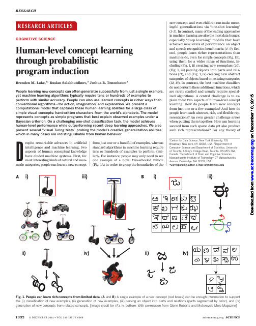
信息检索课程中的英文简称Information Retrieval Course: An In-Depth Exploration.Information retrieval, commonly abbreviated as IR, is a crucial field in computer science that deals with the retrieval of information from large collections of unstructured or semi-structured data. It finds its applications in various domains, including libraries, e-commerce, search engines, and more. In this article, we delve into the intricacies of information retrieval, its importance, and the techniques used in this domain.1. Introduction to Information Retrieval.Information retrieval is the process of obtaining relevant information from a large, often unstructured, collection of data. It involves techniques such as indexing, searching, and ranking to ensure that the most relevant information is presented to the user. The goal is toprovide accurate and timely information to meet the user'sinformation needs.2. Core Components of Information Retrieval.Indexing: Indexing is the process of creating a data structure, such as an inverted index, that maps terms (keywords) to the locations (documents) where they appear. This allows efficient retrieval of documents containing specific terms.Searching: Searching involves the user submitting a query, which is then processed and compared against the index to retrieve relevant documents. Queries can be simple keywords or complex expressions.Ranking: Ranking algorithms determine the order in which retrieved documents are presented to the user. Relevance, popularity, and recency are common factors considered in ranking.3. Types of Information Retrieval Systems.Boolean Retrieval: Boolean retrieval systems allow users to specify search queries using Boolean operators (AND, OR, NOT) to combine terms and filter results.Vector Space Models: These models represent documents and queries as vectors in a high-dimensional space. Relevance is determined by measuring the similarity between these vectors.Probabilistic Models: Probabilistic models estimate the probability of a document being relevant to a given query. They consider factors like term frequencies and document lengths.Learning-to-Rank (L2R) Models: These models use machine learning techniques to learn the ranking function based on training data. They aim to optimize ranking metrics like mean reciprocal rank (MRR) or normalized discounted cumulative gain (NDCG).4. Challenges in Information Retrieval.Semantic Gap: The semantic gap refers to the mismatch between the user's information need and the representationof information in the system. Addressing this gap requires techniques like latent semantic indexing or word embeddings.Scalability: As data collections grow, it becomes challenging to maintain and query the index efficiently. Distributed retrieval systems and近似算法can help address scalability issues.User Intent Understanding: Understanding the trueintent behind a user's query is crucial for accurate retrieval. Techniques like query reformulation and user profiling can aid in understanding user intent.5. Applications of Information Retrieval.Search Engines: Search engines are the most visible application of information retrieval, serving billions of queries daily. They use a combination of IR techniques to provide relevant search results.E-commerce: E-commerce platforms rely on IR to help users find products or services that meet their needs. This involves searching product descriptions, user reviews, and more.Libraries and Archives: Libraries and archives use IR systems to catalog and retrieve books, documents, and other materials. These systems often incorporate metadata and faceted search to enhance retrieval accuracy.Question Answering Systems: Question answering systems aim to provide direct answers to user queries, often by analyzing a large corpus of text to extract relevant information.6. Future Trends in Information Retrieval.Semantic Retrieval: As the focus shifts towards understanding the true meaning of queries and documents, semantic retrieval techniques like entity linking and semantic role labeling will become increasingly important.Multimodal Retrieval: With the increasing availability of multimedia content, there is a growing need for systems that can handle text, images, audio, and video simultaneously.Personalized Retrieval: Techniques like user profiling and collaborative filtering will play a crucial role in personalizing search results based on user preferences and behavior.Interactive Retrieval: Systems that allow users to interactively refine their queries or provide feedback on search results will improve retrieval accuracy and user satisfaction.In conclusion, information retrieval is a crucial field that powers many of the technologies we rely on daily. It involves complex techniques and algorithms to ensure accurate and timely information delivery. As data volumes continue to grow and user needs become more sophisticated, IR research will focus on addressing challenges like the semantic gap, scalability, and user intent understanding.Future trends like semantic retrieval, multimodal retrieval, personalized retrieval, and interactive retrieval will further enhance the capabilities of IR systems and improve user experiences.。

Networked ModelsSchool of Electronic and Computer EngineeringPeking UniversityWang Wenmin12. Models in Machine Learning Contents:☐12.1. Probabilistic Models☐12.2. Geometric Models☐12.3. Logical Models☐12.4. Networked Models12.4. Networked Models What are Networked Models 什么是网络化模型☐The networked models here refer to as the models of artificial neural network(ANN).这里的网络化模型指的是人工神经网络模型(ANN)。

☐An ANN is an artificial representation of the human brain that tries to simulate its learning processing.一个ANN是人脑的一种人工表征，试图模拟人类的学习过程。

☐ANN can be constructed a system by interconnected “neurons” which send messages to each other.ANN可以通过互联的“神经元”构建一个系统，神经元之间相互发送消息。

☐The connections between neurons have numeric weights that can be tuned based on experience, making ANN adaptive to inputs and capable of learning.神经元之间的连接具有数值权重，可以通过经验调整，使ANN适应输入并且能够学习。