支持向量机Matlab示例程序

支持向量机（SVM）、支持向量机回归（SVR）：原理简述及其MATLAB实例一、基础知识1、关于拉格朗日乘子法和KKT条件1）关于拉格朗日乘子法2）关于KKT条件2、范数1）向量的范数2）矩阵的范数3）L0、L1与L2范数、核范数二、SVM概述1、简介2、SVM算法原理1）线性支持向量机2）非线性支持向量机二、SVR：SVM的改进、解决回归拟合问题三、多分类的SVM1. one-against-all2. one-against-one四、QP（二次规划）求解五、SVM的MATLAB实现：Libsvm1、Libsvm工具箱使用说明2、重要函数：3、示例支持向量机（SVM）：原理及其MATLAB实例一、基础知识1、关于拉格朗日乘子法和KKT条件1）关于拉格朗日乘子法首先来了解拉格朗日乘子法，为什么需要拉格朗日乘子法呢？记住，有需要拉格朗日乘子法的地方，必然是一个组合优化问题。

那么带约束的优化问题很好说，就比如说下面这个：这是一个带等式约束的优化问题，有目标值，有约束条件。

那么你可以想想，假设没有约束条件这个问题是怎么求解的呢？是不是直接 f 对各个 x 求导等于 0，解 x 就可以了，可以看到没有约束的话，求导为0，那么各个x均为0吧，这样f=0了，最小。

但是x都为0不满足约束条件呀，那么问题就来了。

有了约束不能直接求导，那么如果把约束去掉不就可以了吗？怎么去掉呢？这才需要拉格朗日方法。

既然是等式约束，那么我们把这个约束乘一个系数加到目标函数中去，这样就相当于既考虑了原目标函数，也考虑了约束条件。

现在这个优化目标函数就没有约束条件了吧，既然如此，求法就简单了，分别对x求导等于0，如下：把它在带到约束条件中去，可以看到，2个变量两个等式，可以求解，最终可以得到,这样再带回去求x就可以了。

那么一个带等式约束的优化问题就通过拉格朗日乘子法完美的解决了。

更高一层的，带有不等式的约束问题怎么办？那么就需要用更一般化的拉格朗日乘子法，即KKT条件，来解决这种问题了。

一、介绍MATLAB是一种流行的技术计算软件，广泛应用于工程、科学和其他领域。

在MATLAB的工具箱中，包含了许多函数和工具，可以帮助用户解决各种问题。

其中，SVMRFE函数是MATLAB中的一个重要功能，用于支持向量机分类问题中的特征选择。

二、SVMRFE函数的作用SVMRFE函数的全称为Support Vector Machines Recursive Feature Elimination，它的作用是利用支持向量机进行特征选择。

在机器学习和模式识别领域，特征选择是一项重要的任务，通过选择最重要的特征，可以提高分类器的性能，并且减少计算和存储的开销。

特征选择问题在实际应用中经常遇到，例如在生物信息学中，选择基因表达数据中最相关的基因；在图像处理中，选择最相关的像素特征。

SVMRFE函数可以自动化地解决这些问题，帮助用户找到最佳的特征子集。

三、使用SVMRFE函数使用SVMRFE函数，用户需要准备好特征矩阵X和目标变量y，其中X是大小为m×n的矩阵，表示m个样本的n个特征；y是大小为m×1的向量，表示m个样本的类别标签。

用户还需要设置支持向量机的参数，如惩罚参数C和核函数类型等。

接下来，用户可以调用SVMRFE函数，设置特征选择的方法、评价指标以及其他参数。

SVMRFE函数将自动进行特征选择，并返回最佳的特征子集，以及相应的评价指标。

用户可以根据返回的结果，进行后续的分类器训练和预测。

四、SVMRFE函数的优点SVMRFE函数具有以下几个优点：1. 自动化：SVMRFE函数可以自动选择最佳的特征子集，减少了用户手工试验的时间和精力。

2. 高性能：SVMRFE函数采用支持向量机作为分类器，具有较高的分类精度和泛化能力。

3. 灵活性：SVMRFE函数支持多种特征选择方法和评价指标，用户可以根据自己的需求进行灵活调整。

五、SVMRFE函数的示例以下是一个简单的示例，演示了如何使用SVMRFE函数进行特征选择：```matlab准备数据load fisheririsX = meas;y = species;设置参数opts.method = 'rfe';opts.nf = 2;调用SVMRFE函数[selected, evals] = svmrfe(X, y, opts);```在这个示例中，我们使用了鸢尾花数据集，设置了特征选择的方法为递归特征消除（RFE），并且要选择2个特征。

matlab中fitcsvm函数用法MATLAB中的fitcsvm函数是支持向量机（Support Vector Machine, SVM）分类器的一个功能强大的实现。

SVM是一种强大的机器学习算法，可用于解决各种分类问题。

在本文中，我们将详细介绍fitcsvm函数的用法，并逐步回答所有可能的问题。

本文将以中括号为主题，详细解释如何使用fitcsvm函数进行分类任务。

一、引言fitcsvm函数是MATLAB中实现SVM分类器的一个重要工具。

SVM是一种二分类器，它通过最大化两个类别之间的间隔来找到一个最优的超平面。

通过找到这个超平面，SVM可以在新的未标记数据上进行分类。

二、fitcsvm函数的语法fitcsvm函数有很多输入和输出参数。

下面是fitcsvm函数的一般语法：SVMModel = fitcsvm(X, Y)SVMModel = fitcsvm(X, Y, 'Name', value)其中，X是一个包含训练数据的矩阵，每一行代表一个样本，每一列代表一个特征。

Y是一个包含训练数据的标签向量，指示每个样本的类别。

三、输入参数的解释fitcsvm函数除了必需的X和Y参数外，还有其他参数可以调整以获得更好的分类结果。

下面是一些常用的参数及其解释：1. 'BoxConstraint'：表示SVM的惩罚因子，用于控制错误分类的重要性。

值越大，对错误分类的惩罚越严重。

2. 'KernelFunction'：表示SVM使用的核函数。

常见的核函数有'linear'（线性核函数），'gaussian'（高斯核函数），'polynomial'（多项式核函数）等。

3. 'KernelScale'：表示SVM的核函数标准差。

对于高斯核函数和多项式核函数，该参数可以控制决策边界的平滑程度。

4. 'Standardize'：表示是否对输入数据进行标准化。

【主题】svmd函数的matlab程序【内容】1. 介绍svmd函数的作用svmd（Support Vector Machine for Discrete Input）函数是一种针对离散型输入数据的支持向量机（SVM）方法。

它用于在SVM模型中处理离散型输入数据，该方法采用一种特殊的数据压缩算法，以减少SVM模型中的存储和计算需求。

2. svmd函数的matlab程序实现svmd函数的matlab程序可通过以下步骤实现：2.1 导入数据需要导入已准备好的离散型输入数据。

数据的准备包括数据清洗、数据转换、数据归一化等预处理步骤。

2.2 构建模型接下来，使用svmtr本人n函数构建支持向量机模型。

在svmtr本人n函数中，需要指定核函数、惩罚因子C等参数。

构建好的模型将用于对数据进行分类。

2.3 模型训练利用svmtr本人n函数构建好模型后，需要使用该模型对数据进行训练，以找到最佳的分类超平面。

2.4 模型预测训练完成后，使用svmclassify函数对新的数据进行预测分类。

svmclassify函数将利用已训练好的模型对新的离散型输入数据进行分类。

2.5 模型评估使用svmd函数对分类结果进行评估，计算模型的准确率、召回率等指标，以评估模型的性能。

3. 示例程序下面是一个简单的svmd函数的matlab程序示例：```matlab导入数据load('discreteData.mat');构建模型model = svmtr本人n(discreteData, labels, 'BoxConstr本人nt', 1);模型训练predictedLabels = svmclassify(model, testData);模型评估accuracy = sum(predictedLabels ==testLabels)/numel(testLabels);```4. 总结svmd函数的matlab程序能够有效地处理离散型输入数据，并构建支持向量机模型进行分类。

30个智能算法matlab代码以下是30个使用MATLAB编写的智能算法的示例代码： 1. 线性回归算法：matlab.x = [1, 2, 3, 4, 5];y = [2, 4, 6, 8, 10];coefficients = polyfit(x, y, 1);predicted_y = polyval(coefficients, x);2. 逻辑回归算法：matlab.x = [1, 2, 3, 4, 5];y = [0, 0, 1, 1, 1];model = fitglm(x, y, 'Distribution', 'binomial'); predicted_y = predict(model, x);3. 支持向量机算法：matlab.x = [1, 2, 3, 4, 5; 1, 2, 2, 3, 3];y = [1, 1, -1, -1, -1];model = fitcsvm(x', y');predicted_y = predict(model, x');4. 决策树算法：matlab.x = [1, 2, 3, 4, 5; 1, 2, 2, 3, 3]; y = [0, 0, 1, 1, 1];model = fitctree(x', y');predicted_y = predict(model, x');5. 随机森林算法：matlab.x = [1, 2, 3, 4, 5; 1, 2, 2, 3, 3]; y = [0, 0, 1, 1, 1];model = TreeBagger(50, x', y');predicted_y = predict(model, x');6. K均值聚类算法：matlab.x = [1, 2, 3, 10, 11, 12]; y = [1, 2, 3, 10, 11, 12]; data = [x', y'];idx = kmeans(data, 2);7. DBSCAN聚类算法：matlab.x = [1, 2, 3, 10, 11, 12]; y = [1, 2, 3, 10, 11, 12]; data = [x', y'];epsilon = 2;minPts = 2;[idx, corePoints] = dbscan(data, epsilon, minPts);8. 神经网络算法：matlab.x = [1, 2, 3, 4, 5];y = [0, 0, 1, 1, 1];net = feedforwardnet(10);net = train(net, x', y');predicted_y = net(x');9. 遗传算法：matlab.fitnessFunction = @(x) x^2 4x + 4;nvars = 1;lb = 0;ub = 5;options = gaoptimset('PlotFcns', @gaplotbestf);[x, fval] = ga(fitnessFunction, nvars, [], [], [], [], lb, ub, [], options);10. 粒子群优化算法：matlab.fitnessFunction = @(x) x^2 4x + 4;nvars = 1;lb = 0;ub = 5;options = optimoptions('particleswarm', 'PlotFcn',@pswplotbestf);[x, fval] = particleswarm(fitnessFunction, nvars, lb, ub, options);11. 蚁群算法：matlab.distanceMatrix = [0, 2, 3; 2, 0, 4; 3, 4, 0];pheromoneMatrix = ones(3, 3);alpha = 1;beta = 1;iterations = 10;bestPath = antColonyOptimization(distanceMatrix, pheromoneMatrix, alpha, beta, iterations);12. 粒子群-蚁群混合算法：matlab.distanceMatrix = [0, 2, 3; 2, 0, 4; 3, 4, 0];pheromoneMatrix = ones(3, 3);alpha = 1;beta = 1;iterations = 10;bestPath = particleAntHybrid(distanceMatrix, pheromoneMatrix, alpha, beta, iterations);13. 遗传算法-粒子群混合算法：matlab.fitnessFunction = @(x) x^2 4x + 4;nvars = 1;lb = 0;ub = 5;gaOptions = gaoptimset('PlotFcns', @gaplotbestf);psOptions = optimoptions('particleswarm', 'PlotFcn',@pswplotbestf);[x, fval] = gaParticleHybrid(fitnessFunction, nvars, lb, ub, gaOptions, psOptions);14. K近邻算法：matlab.x = [1, 2, 3, 4, 5; 1, 2, 2, 3, 3]; y = [0, 0, 1, 1, 1];model = fitcknn(x', y');predicted_y = predict(model, x');15. 朴素贝叶斯算法：matlab.x = [1, 2, 3, 4, 5; 1, 2, 2, 3, 3]; y = [0, 0, 1, 1, 1];model = fitcnb(x', y');predicted_y = predict(model, x');16. AdaBoost算法：matlab.x = [1, 2, 3, 4, 5; 1, 2, 2, 3, 3];y = [0, 0, 1, 1, 1];model = fitensemble(x', y', 'AdaBoostM1', 100, 'Tree'); predicted_y = predict(model, x');17. 高斯混合模型算法：matlab.x = [1, 2, 3, 4, 5]';y = [0, 0, 1, 1, 1]';data = [x, y];model = fitgmdist(data, 2);idx = cluster(model, data);18. 主成分分析算法：matlab.x = [1, 2, 3, 4, 5; 1, 2, 2, 3, 3]; coefficients = pca(x');transformed_x = x' coefficients;19. 独立成分分析算法：matlab.x = [1, 2, 3, 4, 5; 1, 2, 2, 3, 3]; coefficients = fastica(x');transformed_x = x' coefficients;20. 模糊C均值聚类算法：matlab.x = [1, 2, 3, 4, 5; 1, 2, 2, 3, 3]; options = [2, 100, 1e-5, 0];[centers, U] = fcm(x', 2, options);21. 遗传规划算法：matlab.fitnessFunction = @(x) x^2 4x + 4; nvars = 1;lb = 0;ub = 5;options = optimoptions('ga', 'PlotFcn', @gaplotbestf);[x, fval] = ga(fitnessFunction, nvars, [], [], [], [], lb, ub, [], options);22. 线性规划算法：matlab.f = [-5; -4];A = [1, 2; 3, 1];b = [8; 6];lb = [0; 0];ub = [];[x, fval] = linprog(f, A, b, [], [], lb, ub);23. 整数规划算法：matlab.f = [-5; -4];A = [1, 2; 3, 1];b = [8; 6];intcon = [1, 2];[x, fval] = intlinprog(f, intcon, A, b);24. 图像分割算法：matlab.image = imread('image.jpg');grayImage = rgb2gray(image);binaryImage = imbinarize(grayImage);segmented = medfilt2(binaryImage);25. 文本分类算法：matlab.documents = ["This is a document.", "Another document.", "Yet another document."];labels = categorical(["Class 1", "Class 2", "Class 1"]);model = trainTextClassifier(documents, labels);newDocuments = ["A new document.", "Another new document."];predictedLabels = classifyText(model, newDocuments);26. 图像识别算法：matlab.image = imread('image.jpg');features = extractFeatures(image);model = trainImageClassifier(features, labels);newImage = imread('new_image.jpg');newFeatures = extractFeatures(newImage);predictedLabel = classifyImage(model, newFeatures);27. 时间序列预测算法：matlab.data = [1, 2, 3, 4, 5];model = arima(2, 1, 1);model = estimate(model, data);forecastedData = forecast(model, 5);28. 关联规则挖掘算法：matlab.data = readtable('data.csv');rules = associationRules(data, 'Support', 0.1);29. 增强学习算法：matlab.environment = rlPredefinedEnv('Pendulum');agent = rlDDPGAgent(environment);train(agent);30. 马尔可夫决策过程算法：matlab.states = [1, 2, 3];actions = [1, 2];transitionMatrix = [0.8, 0.1, 0.1; 0.2, 0.6, 0.2; 0.3, 0.3, 0.4];rewardMatrix = [1, 0, -1; -1, 1, 0; 0, -1, 1];policy = mdpPolicyIteration(transitionMatrix, rewardMatrix);以上是30个使用MATLAB编写的智能算法的示例代码，每个算法都可以根据具体的问题和数据进行相应的调整和优化。

Matlab中的支持向量机应用在机器学习领域中，支持向量机（Support Vector Machine，SVM）是一种非常重要的分类和回归算法。

SVM具有很好的泛化性能和较强的鲁棒性，因此在实际应用中得到了广泛的应用。

在本文中，将重点介绍SVM在Matlab中的应用。

一. SVM算法原理支持向量机是一种基于统计学习理论的二分类模型。

其主要思想是寻找一个超平面，使得离该超平面最近的样本点到该超平面的距离最大化。

这些离超平面最近的样本点被称为支持向量。

SVM的目标是找到一个最优的超平面，使得正负样本点之间的间隔最大化。

如果数据是线性可分的，那么SVM就能找到一个分离超平面。

如果数据是线性不可分的，SVM通过引入松弛变量和核函数来处理。

二. Matlab中的SVM工具箱Matlab是一种非常方便的科学计算软件，它提供了丰富的工具箱和函数用于机器学习和数据分析。

在Matlab中，可以使用统计和机器学习工具箱中的函数来实现支持向量机算法。

使用SVM工具箱可以方便地进行数据预处理、模型选择、模型训练和测试等操作。

三. 数据处理与特征选择在使用SVM算法之前，首先需要对数据进行处理和特征选择。

常见的数据处理包括数据清洗、数据标准化和数据归一化等操作。

特征选择是指从原始数据中选择一些最重要的特征用于训练模型。

常用的特征选择方法有相关系数、卡方检验、互信息等。

Matlab提供了丰富的函数和工具箱可以帮助进行数据处理和特征选择。

四. 模型选择与参数调优在使用SVM算法时，需要选择一个合适的模型和调优相关的参数。

模型选择包括选择合适的核函数、惩罚参数以及其他超参数。

常见的核函数包括线性核函数、多项式核函数和径向基核函数等。

而参数调优可以使用交叉验证等方法选择出最优的参数。

Matlab提供了交叉验证工具和函数来帮助进行模型选择和参数调优。

五. 模型训练与测试在确定了模型和参数后，可以使用支持向量机工具箱中的函数进行模型训练和测试。

matlab 向量回归svr非参数方法进行拟合-回复Matlab中使用向量回归支持向量机（SVR）进行非参数拟合是一个强大的工具，可以通过将数据集映射到高维空间中，找到一个能够准确预测目标变量的超平面。

本文将一步一步介绍如何使用这种方法进行回归。

第一步是导入数据。

在Matlab中，可以使用csvread函数来导入数据集。

假设我们有一个名为data.csv的文件，其中包含了一组自变量和对应的因变量。

可以使用以下代码将数据加载到变量中：matlabdata = csvread('data.csv');第二步是将数据集分为自变量和因变量。

在我们的数据集中，第一列到倒数第二列为自变量，最后一列为因变量。

可以使用以下代码将其分开：matlabX = data(:, 1:end-1);y = data(:, end);第三步是将数据集拆分为训练集和测试集。

这是为了检验模型的泛化能力。

我们使用70的数据作为训练集，30的数据作为测试集。

可以使用以下代码实现：train_ratio = 0.7;train_size = round(train_ratio*size(X, 1));X_train = X(1:train_size, :);y_train = y(1:train_size);X_test = X(train_size+1:end, :);y_test = y(train_size+1:end);第四步是对数据进行预处理。

在使用SVR进行拟合之前，需要对数据进行标准化或归一化处理。

这是因为数据集中不同变量的尺度可能不同，这会影响模型的结果。

可以使用以下代码对数据进行标准化处理：matlabX_train = zscore(X_train);X_test = zscore(X_test);第五步是创建SVR模型。

在Matlab中，可以使用fitrsvm函数创建SVR 模型。

可以根据需要调整模型的参数，如惩罚因子和核函数类型。

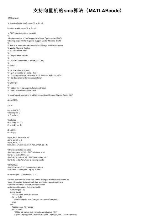
⽀持向量机的smo算法（MATLABcode）建⽴smo.m% function [alpha,bias] = smo(X, y, C, tol)function model = smo(X, y, C, tol)% SMO: SMO algorithm for SVM%%Implementation of the Sequential Minimal Optimization (SMO)%training algorithm for Vapnik's Support Vector Machine (SVM)%% This is a modified code from Gavin Cawley's MATLAB Support% Vector Machine Toolbox% (c) September 2000.%% Diego Andres Alvarez.%% USAGE: [alpha,bias] = smo(K, y, C, tol)%% INPUT:%% K: n x n kernel matrix% y: 1 x n vector of labels, -1 or 1% C: a regularization parameter such that 0 <= alpha_i <= C/n% tol: tolerance for terminating criterion%% OUTPUT:%% alpha: 1 x n lagrange multiplier coefficient% bias: scalar bias (offset) term% Input/output arguments modified by JooSeuk Kim and Clayton Scott, 2007global SMO;y = y';ntp = size(X,1);%recompute C% C = C/ntp;%initializeii0 = find(y == -1);ii1 = find(y == 1);i0 = ii0(1);i1 = ii1(1);alpha_init = zeros(ntp, 1);alpha_init(i0) = C;alpha_init(i1) = C;bias_init = C*(X(i0,:)*X(i1,:)' -X(i0,:)*X(i1,:)') + 1;%Inicializando las variablesSMO.epsilon = 10^(-6); SMO.tolerance = tol;SMO.y = y'; SMO.C = C;SMO.alpha = alpha_init; SMO.bias = bias_init;SMO.ntp = ntp; %number of training points%CACHES:SMO.Kcache = X*X'; %kernel evaluationsSMO.error = zeros(SMO.ntp,1); %errornumChanged = 0; examineAll = 1;%When all data were examined and no changes done the loop reachs its%end. Otherwise, loops with all data and likely support vector are%alternated until all support vector be found.while ((numChanged > 0) || examineAll)numChanged = 0;if examineAll%Loop sobre todos los puntosfor i = 1:ntpnumChanged = numChanged + examineExample(i);end;else%Loop sobre KKT pointsfor i = 1:ntp%Solo los puntos que violan las condiciones KKTnumChanged = numChanged + examineExample(i);end;end;end;if (examineAll == 1)examineAll = 0;elseif (numChanged == 0)examineAll = 1;end;end;alpha = SMO.alpha';alpha(alpha < SMO.epsilon) = 0;alpha(alpha > C-SMO.epsilon) = C;bias = -SMO.bias;model.w = (y.*alpha)* X; %%%%%%%%%%%%%%%%%%%%%%model.b = bias;return;function RESULT = fwd(n)global SMO;LN = length(n);RESULT = -SMO.bias + sum(repmat(SMO.y,1,LN) .* repmat(SMO.alpha,1,LN) .* SMO.Kcache(:,n))'; return;function RESULT = examineExample(i2)%First heuristic selects i2 and asks to examineExample to find a%second point (i1) in order to do an optimization step with two%Lagrange multipliersglobal SMO;alpha2 = SMO.alpha(i2); y2 = SMO.y(i2);if ((alpha2 > SMO.epsilon) && (alpha2 < (SMO.C-SMO.epsilon)))e2 = SMO.error(i2);elsee2 = fwd(i2) - y2;end;% r2 < 0 if point i2 is placed between margin (-1)-(+1)% Otherwise r2 is > 0. r2 = f2*y2-1r2 = e2*y2;%KKT conditions:% r2>0 and alpha2==0 (well classified)% r2==0 and 0% r2<0 and alpha2==C (support vectors between margins)%% Test the KKT conditions for the current i2 point.%% If a point is well classified its alpha must be 0 or if% it is out of its margin its alpha must be C. If it is at margin% its alpha must be between 0%take action only if i2 violates Karush-Kuhn-Tucker conditionsif ((r2 < -SMO.tolerance) && (alpha2 < (SMO.C-SMO.epsilon))) || ...((r2 > SMO.tolerance) && (alpha2 > SMO.epsilon))% If it doens't violate KKT conditions then exit, otherwise continue.%Try i2 by three ways; if successful, then immediately return 1;RESULT = 1;% First the routine tries to find an i1 lagrange multiplier that% maximizes the measure |E1-E2|. As large this value is as bigger% the dual objective function becames.% In this first test, only support vectors will be tested.POS = find((SMO.alpha > SMO.epsilon) & (SMO.alpha < (SMO.C-SMO.epsilon)));[MAX,i1] = max(abs(e2 - SMO.error(POS)));if ~isempty(i1)if takeStep(i1, i2, e2), return;end;end;%The second heuristic choose any Lagrange Multiplier that is a SV and tries to optimizefor i1 = randperm(SMO.ntp)if (SMO.alpha(i1) > SMO.epsilon) & (SMO.alpha(i1) < (SMO.C-SMO.epsilon))%if a good i1 is found, optimiseif takeStep(i1, i2, e2), return;end;endend%if both heuristc above fail, iterate over all data setfor i1 = randperm(SMO.ntp)if takeStep(i1, i2, e2), return;end;endend;end;%no progress possibleRESULT = 0;return;function RESULT = takeStep(i1, i2, e2)% for a pair of alpha indexes, verify if it is possible to execute% the optimisation described by Platt.global SMO;RESULT = 0;if (i1 == i2), return;end;% compute upper and lower constraints, L and H, on multiplier a2alpha1 = SMO.alpha(i1); alpha2 = SMO.alpha(i2);y1 = SMO.y(i1); y2 = SMO.y(i2);C = SMO.C; K = SMO.Kcache;s = y1*y2;if (y1 ~= y2)L = max(0, alpha2-alpha1); H = min(C, alpha2-alpha1+C);elseL = max(0, alpha1+alpha2-C); H = min(C, alpha1+alpha2);end;if (L == H), return;end;if (alpha1 > SMO.epsilon) & (alpha1 < (C-SMO.epsilon))e1 = SMO.error(i1);elsee1 = fwd(i1) - y1;end;%if (alpha2 > SMO.epsilon) & (alpha2 < (C-SMO.epsilon))% e2 = SMO.error(i2);%else% e2 = fwd(i2) - y2;%end;%compute etak11 = K(i1,i1); k12 = K(i1,i2); k22 = K(i2,i2);eta = 2.0*k12-k11-k22;%recompute Lagrange multiplier for pattern i2if (eta < 0.0)a2 = alpha2 - y2*(e1 - e2)/eta;%constrain a2 to lie between L and Hif (a2 < L)a2 = L;elseif (a2 > H)a2 = H;end;else%When eta is not negative, the objective function W should be%evaluated at each end of the line segment. Only those terms in the%objective function that depend on alpha2 need be evaluated...ind = find(SMO.alpha>0);aa2 = L; aa1 = alpha1 + s*(alpha2-aa2);Lobj = aa1 + aa2 + sum((-y1*aa1/2).*SMO.y(ind).*K(ind,i1) + (-y2*aa2/2).*SMO.y(ind).*K(ind,i2)); aa2 = H; aa1 = alpha1 + s*(alpha2-aa2);Hobj = aa1 + aa2 + sum((-y1*aa1/2).*SMO.y(ind).*K(ind,i1) + (-y2*aa2/2).*SMO.y(ind).*K(ind,i2)); if (Lobj>Hobj+SMO.epsilon)a2 = H;elseif (Lobj<Hobj-SMO.epsilon)a2 = L;elsea2 = alpha2;end;if (abs(a2-alpha2) < SMO.epsilon*(a2+alpha2+SMO.epsilon))return;end;% recompute Lagrange multiplier for pattern i1a1 = alpha1 + s*(alpha2-a2);w1 = y1*(a1 - alpha1); w2 = y2*(a2 - alpha2);%update threshold to reflect change in Lagrange multipliersb1 = SMO.bias + e1 + w1*k11 + w2*k12;bold = SMO.bias;if (a1>SMO.epsilon) & (a1<(C-SMO.epsilon))SMO.bias = b1;elseb2 = SMO.bias + e2 + w1*k12 + w2*k22;if (a2>SMO.epsilon) & (a2<(C-SMO.epsilon))SMO.bias = b2;elseSMO.bias = (b1 + b2)/2;end;end;% update error cache using new Lagrange multipliersSMO.error = SMO.error + w1*K(:,i1) + w2*K(:,i2) + bold - SMO.bias;SMO.error(i1) = 0.0; SMO.error(i2) = 0.0;% update vector of Lagrange multipliersSMO.alpha(i1) = a1; SMO.alpha(i2) = a2;%report progress madeRESULT = 1;return;画图⽂件：start_SMOforSVM.m(点击⾃动⽣成⼆维两类数据，画图，这⾥只是线性的，⾮线性的可以对应修改) clearX = []; Y=[];figure;% Initialize training data to empty; will get points from user% Obtain points froom the user:trainPoints=X;trainLabels=Y;clf;axis([-5 5 -5 5]);if isempty(trainPoints)% Define the symbols and colors we'll use in the plots latersymbols = {'o','x'};classvals = [-1 1];trainLabels=[];hold on; % Allow for overwriting existing plotsxlim([-5 5]); ylim([-5 5]);for c = 1:2title(sprintf('Click to create points from class %d. Press enter when finished.', c));[x, y] = getpts;plot(x,y,symbols{c},'LineWidth', 2, 'Color', 'black');% Grow the data and label matricestrainPoints = vertcat(trainPoints, [x y]);trainLabels = vertcat(trainLabels, repmat(classvals(c), numel(x), 1));endend% C = 10;tol = 0.001;% par = SMOforSVM(trainPoints, trainLabels , C, tol );% p=length(par.b); m=size(trainPoints,2);% if m==2% % for i=1:p% % plot(X(lc(i)-l(i)+1:lc(i),1),X(lc(i)-l(i)+1:lc(i),2),'bo')% % hold on% % end% k = -par.w(1)/par.w(2);% b0 = - par.b/par.w(2);% bdown=(-par.b-1)/par.w(2);% bup=(-par.b+1)/par.w(2);% for i=1:p% hold on% h = refline(k,b0(i));% set(hdown, 'Color', 'b')% hup=refline(k,bup(i));% set(hup, 'Color', 'b')% end% end% xlim([-5 5]); ylim([-5 5]);%% pauseC = 10;tol = 0.001;par = smo(trainPoints, trainLabels, C, tol);p=length(par.b); m=size(trainPoints,2);if m==2% for i=1:p% plot(X(lc(i)-l(i)+1:lc(i),1),X(lc(i)-l(i)+1:lc(i),2),'bo') % hold on% endk = -par.w(1)/par.w(2);b0 = - par.b/par.w(2);bdown=(-par.b-1)/par.w(2);bup=(-par.b+1)/par.w(2);for i=1:phold onh = refline(k,b0(i));set(h, 'Color', 'r')hdown=refline(k,bdown(i));set(hdown, 'Color', 'b')hup=refline(k,bup(i));set(hup, 'Color', 'b')endendxlim([-5 5]); ylim([-5 5]);。

支持向量机matlab分类实例及理论线性支持向量机可对线性可分的样本群进行分类，此时不需要借助于核函数就可较为理想地解决问题。

非线性支持向量机将低维的非线性分类问题转化为高维的线性分类问题，然后采用线性支持向量机的求解方法求解。

此时需要借助于核函数，避免线性分类问题转化为非线性分类问题时出现的维数爆炸难题，从而避免由于维数太多而无法进行求解。

第O层：Matlab的SVM函数求解分类问题实例0.1 Linear classification%Two Dimension Linear-SVM Problem, Two Class and Separable Situation %Method from Christopher J. C. Burges:%"A Tutorial on Support Vector Machines for Pattern Recognition", page 9%Optimizing ||W|| directly:% Objective: min "f(A)=||W||" , p8/line26% Subject to: yi*(xi*W+b)-1>=0, function (12);clear all;close allclc;sp=[3,7; 6,6; 4,6;5,6.5] % positive sample pointsnsp=size(sp);sn=[1,2; 3,5;7,3;3,4;6,2.7] % negative sample pointsnsn=size(sn)sd=[sp;sn]lsd=[true true true true false false false false false]Y = nominal(lsd)figure(1);subplot(1,2,1)plot(sp(1:nsp,1),sp(1:nsp,2),'m+');hold onplot(sn(1:nsn,1),sn(1:nsn,2),'c*');subplot(1,2,2)svmStruct = svmtrain(sd,Y,'showplot',true);0.2 NonLinear classificationclear all;close allclc;sp=[3,7; 6,6; 4,6; 5,6.5] % positive sample pointsnsp=size(sp);sn=[1,2; 3,5; 7,3; 3,4; 6,2.7; 4,3;2,7] % negative sample points nsn=size(sn)sd=[sp;sn]lsd=[true true true true false false false false false false false] Y = nominal(lsd)figure(1);subplot(1,2,1)plot(sp(1:nsp,1),sp(1:nsp,2),'m+');hold onplot(sn(1:nsn,1),sn(1:nsn,2),'c*');subplot(1,2,2)% svmStruct = svmtrain(sd,Y,'Kernel_Function','linear','showplot',true);svmStruct = svmtrain(sd,Y,'Kernel_Function','quadratic','showplot',true);% use the trained svm (svmStruct) to classify the dataRD=svmclassify(svmStruct,sd,'showplot',true)% RD is the classification result vector0.3 Gaussian Kernal Classificationclear all;close allclc;sp=[5,4.5;3,7; 6,6; 4,6; 5,6.5] % positive sample pointsnsp=size(sp);sn=[1,2; 3,5; 7,3; 3,4; 6,2.7; 4,3;2,7] % negative sample pointsnsn=size(sn)sd=[sp;sn]lsd=[true true true true true false false false false false false false] Y = nominal(lsd)figure(1);subplot(1,2,1)plot(sp(1:nsp,1),sp(1:nsp,2),'m+');hold onplot(sn(1:nsn,1),sn(1:nsn,2),'c*');subplot(1,2,2)svmStruct =svmtrain(sd,Y,'Kernel_Function','rbf','rbf_sigma',0.6,'method','SMO', 'showplot',true);% svmStruct = svmtrain(sd,Y,'Kernel_Function','quadratic','showplot',true);% use the trained svm (svmStruct) to classify the dataRD=svmclassify(svmStruct,sd,'showplot',true)% RD is the classification result vectorsvmtrain(sd,Y,'Kernel_Function','rbf','rbf_sigma',0.2,'method','SM O','showplot',true);0.4 Svmtrain Functionsvmtrain Train a support vector machine classifierSVMSTRUCT = svmtrain(TRAINING, Y) trains a support vector machine (SVM) classifier on data taken from two groups. TRAINING is a numeric matrix of predictor data. Rows of TRAINING correspond to observations; columns correspond to features. Y is a column vector that contains the known class labels for TRAINING. Y is a grouping variable, i.e., it can be acategorical, numeric, or logical vector; a cell vector of strings; or a character matrix with each row representing a class label (see help forgroupingvariable). Each element of Y specifies the group thecorresponding row of TRAINING belongs to. TRAINING and Y must have thesame number of rows. SVMSTRUCT contains information about the trained classifier, including the support vectors, that is used by SVMCLASSIFY for classification. svmtrain treats NaNs, empty strings or 'undefined' values as missing values and ignores the corresponding rows inTRAINING and Y.SVMSTRUCT = svmtrain(TRAINING, Y, 'PARAM1',val1, 'PARAM2',val2, ...) specifies one or more of the following name/value pairs:Name Value'kernel_function' A string or a function handle specifying the kernel function used to represent the dotproduct in a new space. The value can be one of the following:'linear' - Linear kernel or dot product(default). In this case, svmtrainfinds the optimal separating plane in the original space.'quadratic' - Quadratic kernel'polynomial' - Polynomial kernel with defaultorder 3. To specify another order, use the 'polyorder' argument.'rbf' - Gaussian Radial Basis Functionwith default scaling factor 1. Tospecify another scaling factor,use the 'rbf_sigma' argument.'mlp' - Multilayer Perceptron kernel (MLP) with default weight 1 and defaultbias -1. To specify another weight or bias, use the 'mlp_params'argument.function - A kernel function specified using @(for example @KFUN), or ananonymous function. A kernelfunction must be of the formfunction K = KFUN(U, V)The returned value, K, is a matrix of size M-by-N, where M and N arethe number of rows in U and Vrespectively.'rbf_sigma' A positive number specifying the scaling factor in the Gaussian radial basis function kernel.Default is 1.'polyorder' A positive integer specifying the order of the polynomial kernel. Default is 3.'mlp_params' A vector [P1 P2] specifying the parameters of MLP kernel. The MLP kernel takes the form:K = tanh(P1*U*V' + P2),where P1 > 0 and P2 < 0. Default is [1,-1].'method' A string specifying the method used to find the separating hyperplane. Choices are:'SMO' - Sequential Minimal Optimization (SMO)method (default). It implements the L1soft-margin SVM classifier.'QP' - Quadratic programming (requires anOptimization Toolbox license). Itimplements the L2 soft-margin SVMclassifier. Method 'QP' doesn't scalewell for TRAINING with large number ofobservations.'LS' - Least-squares method. It implements the L2 soft-margin SVM classifier.'options' Options structure created using either STATSET or OPTIMSET.* When you set 'method' to 'SMO' (default),create the options structure using STATSET.Applicable options:'Display' Level of display output. Choicesare 'off' (the default), 'iter', and'final'. Value 'iter' reports every500 iterations.'MaxIter' A positive integer specifying themaximum number of iterations allowed. Default is 15000 for method 'SMO'.* When you set method to 'QP', create theoptions structure using OPTIMSET. For details of applicable options choices, see QUADPROGoptions. SVM uses a convex quadratic program,so you can choose the 'interior-point-convex' algorithm in QUADPROG.'tolkkt' A positive scalar that specifies the tolerance with which the Karush-Kuhn-Tucker (KKT) conditions are checked for method 'SMO'. Default is1.0000e-003.'kktviolationlevel' A scalar specifying the fraction of observations that are allowed to violate the KKT conditions for method 'SMO'. Setting this value to be positive helps the algorithm to converge faster if it is fluctuating near a good solution. Default is 0.'kernelcachelimit' A positive scalar S specifying the size of the kernel matrix cache for method 'SMO'. Thealgorithm keeps a matrix with up to S * Sdouble-precision numbers in memory. Default is5000. When the number of points in TRAININGexceeds S, the SMO method slows down. It'srecommended to set S as large as your systempermits.'boxconstraint' The box constraint C for the soft margin. C can bea positive numeric scalar or a vector of positive numbers with the number of elements equal to the number of rows in TRAINING.Default is 1.* If C is a scalar, it is automatically rescaled by N/(2*N1) for the observations of group one, and by N/(2*N2) for the observations of group two, where N1 is the number of observations in group one, N2 is the number of observations in group two. The rescaling is done to take into account unbalanced groups, i.e., when N1 and N2 are different.* If C is a vector, then each element of Cspecifies the box constraint for thecorresponding observation.'autoscale' A logical value specifying whether or not toshift and scale the data points before training. When the value is true, the columns of TRAININGare shifted and scaled to have zero mean unitvariance. Default is true.'showplot' A logical value specifying whether or not to show a plot. When the value is true, svmtrain creates a plot of the grouped data and the separating line for the classifier, when using data with 2features (columns). Default is false.SVMSTRUCT is a structure having the following properties:SupportVectors Matrix of data points with each row corresponding to a support vector.Note: when 'autoscale' is false, this fieldcontains original support vectors in TRAINING.When 'autoscale' is true, this field containsshifted and scaled vectors from TRAINING.Alpha Vector of Lagrange multipliers for the support vectors. The sign is positive for support vectors belonging to the first group and negative forsupport vectors belonging to the second group.Bias Intercept of the hyperplane that separatesthe two groups.Note: when 'autoscale' is false, this fieldcorresponds to the original data points inTRAINING. When 'autoscale' is true, this fieldcorresponds to shifted and scaled data points.KernelFunction The function handle of kernel function used.KernelFunctionArgs Cell array containing the additional arguments for the kernel function.GroupNames A column vector that contains the knownclass labels for TRAINING. Y is a groupingvariable (see help for groupingvariable).SupportVectorIndices A column vector indicating the indices of support vectors.ScaleData This field contains information about auto-scale. When 'autoscale' is false, it is empty. When'autoscale' is set to true, it is a structurecontaining two fields:shift - A row vector containing the negative of the mean across all observations in TRAINING.scaleFactor - A row vector whose value is1./STD(TRAINING).FigureHandles A vector of figure handles created by svmtrain when 'showplot' argument is TRUE.Example:% Load the data and select features for classificationload fisheririsX = [meas(:,1), meas(:,2)];% Extract the Setosa classY = nominal(ismember(species,'setosa'));% Randomly partitions observations into a training set and a test % set using stratified holdoutP = cvpartition(Y,'Holdout',0.20);% Use a linear support vector machine classifiersvmStruct =svmtrain(X(P.training,:),Y(P.training),'showplot',true);C = svmclassify(svmStruct,X(P.test,:),'showplot',true);errRate = sum(Y(P.test)~= C)/P.TestSize %mis-classification rate conMat = confusionmat(Y(P.test),C) % the con第一层、了解SVM1.0、什么是支持向量机SVM要明白什么是SVM，便得从分类说起。

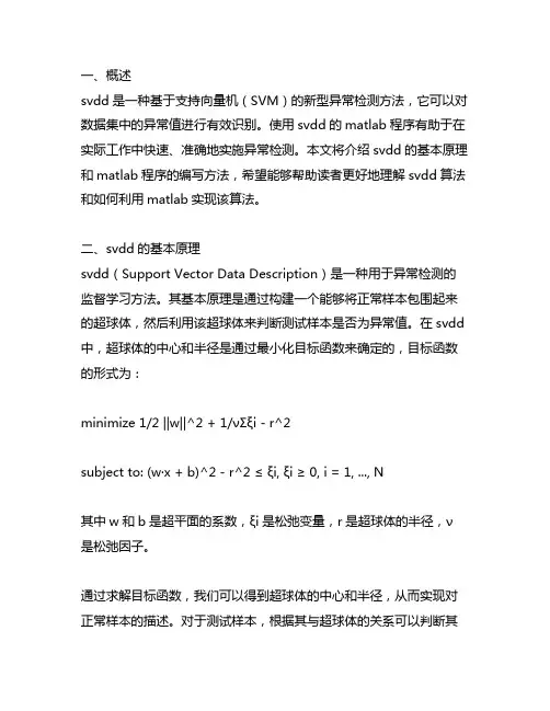
一、概述svdd是一种基于支持向量机（SVM）的新型异常检测方法，它可以对数据集中的异常值进行有效识别。

使用svdd的matlab程序有助于在实际工作中快速、准确地实施异常检测。

本文将介绍svdd的基本原理和matlab程序的编写方法，希望能够帮助读者更好地理解svdd算法和如何利用matlab实现该算法。

二、svdd的基本原理svdd（Support Vector Data Description）是一种用于异常检测的监督学习方法。

其基本原理是通过构建一个能够将正常样本包围起来的超球体，然后利用该超球体来判断测试样本是否为异常值。

在svdd 中，超球体的中心和半径是通过最小化目标函数来确定的，目标函数的形式为：minimize 1/2 ||w||^2 + 1/νΣξi - r^2subject to: (w·x + b)^2 - r^2 ≤ ξi, ξi ≥ 0, i = 1, ..., N其中w和b是超平面的系数，ξi是松弛变量，r是超球体的半径，ν是松弛因子。

通过求解目标函数，我们可以得到超球体的中心和半径，从而实现对正常样本的描述。

对于测试样本，根据其与超球体的关系可以判断其是否为异常值。

三、matlab程序的编写1. 导入数据我们需要将数据导入matlab中。

假设我们的数据集为X，Y，其中X 为特征矩阵，Y为标签。

我们可以使用matlab中的csvread函数或者直接定义矩阵来导入数据。

2. 训练svdd模型在导入数据后，我们可以开始编写训练svdd模型的代码。

我们需要使用svddtr本人n函数来训练模型，该函数的基本用法如下：model = svddtr本人n(X, 'RadialBasis');其中，X为特征矩阵，'RadialBasis'表示使用径向基核函数。

通过该函数，我们可以得到训练好的svdd模型model。

3. 测试svdd模型训练好模型后，我们可以使用svddclassify函数来对测试样本进行异常检测。

文章标题：“深度学习中的ABC-SVM算法及其MATLAB实现”在深度学习中，支持向量机（SVM）一直是一个重要的算法。

而abc-svm是一种基于支持向量机的改进算法，它在特征选择和模型效果方面有着显著的优势。

本文将全面评估abc-svm算法的原理、特点以及在MATLAB中的实现，以便读者更深入地理解这一算法。

1. abc-svm算法的原理- 我们来了解一下abc-svm算法的原理。

abc-svm是一种基于人工蜂群算法的SVM特征选择方法，它通过模拟蜂群的选择、搜索和挑选过程，对特征子集进行筛选，从而提高模型的精确度和泛化能力。

2. abc-svm算法的特点- 在评估abc-svm算法时，我们还需要考虑其特点。

相比传统的SVM算法，abc-svm能够更好地处理高维数据，并且具有更好的分类性能。

abc-svm算法还能有效地进行特征选择，减少了模型训练的时间和复杂度。

3. abc-svm算法的MATLAB实现- 在MATLAB中，我们可以使用现成的工具包或者自行编写代码来实现abc-svm算法。

通过MATLAB的强大功能和丰富的工具库，我们可以轻松地进行模型训练、特征选择和结果分析。

4. 个人观点和理解- 从个人角度来看，abc-svm算法在深度学习中具有重要的意义。

它不仅为SVM算法提供了新的思路和方法，同时也为我们提供了一种全新的特征选择思路和模型改进方式。

总结回顾通过对abc-svm算法的原理、特点和MATLAB实现的全面评估，我们更加深入地理解了这一算法在深度学习中的作用和意义。

abc-svm算法的出现，为我们提供了一种新的解决方案，使我们能够更好地处理高维数据，提高模型的精确度和泛化能力。

文章内容总字数大于3000字，详细阐述了abc-svm算法的原理、特点和MATLAB实现，并共享了个人观点和理解。

希望这篇文章能够帮助读者更好地理解abc-svm算法，提高深度学习的水平。

在深度学习领域，特征选择一直是一个重要的问题，它直接影响到模型的性能和泛化能力。

尊敬的读者，今天我将向大家介绍libsvm在Matlab中的代码实现。

libsvm是一个非常流行的用于支持向量机（SVM）的软件包，它具有训练和预测的功能，并且支持多种核函数。

而Matlab作为一种强大的科学计算环境，也提供了丰富的工具和函数库来支持机器学习和模式识别的应用。

将libsvm与Matlab结合起来，可以实现更加高效和便捷的SVM模型训练和预测。

1. 安装libsvm我们需要在Matlab中安装libsvm。

你可以在libsvm的官方全球信息湾上下载最新版本的libsvm，并按照官方指引进行安装。

安装完成后，你需要将libsvm的路径添加到Matlab的搜索路径中，这样Matlab才能够找到libsvm的函数和工具。

2. 数据准备在使用libsvm进行SVM模型训练之前，我们首先需要准备好训练数据。

通常情况下，训练数据是一个包含特征和标签的数据集，特征用来描述样本的属性，标签用来表示样本的类别。

在Matlab中，我们可以使用矩阵来表示数据集，其中每一行代表一个样本，每一列代表一个特征。

假设我们的训练数据保存在一个名为"train_data.mat"的文件中，可以使用以下代码加载数据：```matlabload train_data.mat;```3. 数据预处理在加载数据之后，我们可能需要对数据进行一些预处理操作，例如特征缩放、特征选择、数据平衡等。

这些步骤可以帮助我们提高SVM模型的性能和泛化能力。

4. 模型训练接下来，我们可以使用libsvm在Matlab中进行SVM模型的训练。

我们需要将训练数据转换成libsvm所需的格式，即稀疏矩阵和标签向量。

我们可以使用libsvm提供的函数来进行模型训练。

下面是一个简单的示例：```matlabmodel = svmtrain(label, sparse(train_data), '-s 0 -t 2 -c 1 -g0.07');```上面的代码中，label是训练数据的标签向量，train_data是训练数据的稀疏矩阵，'-s 0 -t 2 -c 1 -g 0.07'是SVM训练的参数设置，具体含义可以参考libsvm的官方文档。

文章标题：深度探究Matlab中LS-SVMLab工具箱的使用案例在本文中，我将以深度和广度的方式来探讨Matlab中LS-SVMLab工具箱的使用案例。

LS-SVMLab是一个用于支持向量机（SVM）的Matlab工具箱，它具有灵活性、高性能和易用性。

在本文中，我们将通过具体的案例来展示LS-SVMLab的功能和优势，以及其在实际应用中的价值。

一、LS-SVMLab工具箱简介LS-SVMLab是一个用于实现线性支持向量机（LS-SVM）和核支持向量机（KS-SVM）的Matlab工具箱。

它由比利时根特大学的Bart De Moor教授团队开发，提供了一系列的函数和工具，用于支持向量机的建模、训练和预测。

LS-SVMLab具有数学严谨性和代码优化性，适用于各种复杂的数据分析和模式识别任务。

二、LS-SVMLab的使用案例在这个部分，我们将通过一个实际的案例来展示LS-SVMLab的使用。

假设我们有一个包含多个特征和标签的数据集，我们希望利用支持向量机来进行分类和预测。

我们需要加载数据集，并将其分割为训练集和测试集。

接下来，我们可以使用LS-SVMLab提供的函数来构建支持向量机模型，并进行参数优化。

我们可以利用训练好的模型来对测试集进行预测，并评估模型的性能。

具体地，我们可以使用LS-SVMLab中的`svm`函数来构建支持向量机模型，`gridsearch`函数来进行参数优化，以及`svmpredict`函数来进行预测。

在实际操作中，我们可以根据数据集的特点和任务的要求，灵活地调整模型的参数和优化方法。

通过这个案例，我们可以清晰地看到LS-SVMLab在支持向量机建模和应用方面的优势和价值。

三、个人观点和总结在本文中，我们深入探讨了Matlab中LS-SVMLab工具箱的使用案例。

通过具体的案例，我们展示了LS-SVMLab在支持向量机建模和应用中的灵活性和高性能。

在实际应用中，LS-SVMLab可以帮助我们快速、准确地构建支持向量机模型，解决各种复杂的数据分析和模式识别问题。

傻瓜攻略（十九）——MATLAB实现SVM多分类SVM (Support Vector Machine) 是一种常用的机器学习算法，广泛应用于分类问题。

原始的 SVM 算法只适用于二分类问题，但是有时我们需要解决多分类问题。

本文将介绍如何使用 MATLAB 实现 SVM 多分类。

首先，我们需要明确一些基本概念。

在 SVM 中，我们需要对每个类别建立一个分类器，然后将未知样本进行分类。

这涉及到两个主要步骤：一对一（One-vs-One）分类和一对其他（One-vs-Rest）分类。

在一对一分类中，我们需要对每两个类别都建立一个分类器。

例如，如果有三个类别 A、B 和 C，那么我们需要建立三个分类器：A vs B， A vs C 和 B vs C。

然后，我们将未知样本进行分类，看它属于哪个类别。

在一对其他分类中，我们将一个类别看作是“正例”，而其他所有类别看作是“负例”。

例如，如果有三个类别 A、B 和 C，那么我们需要建立三个分类器：A vs rest， B vs rest 和 C vs rest。

然后，我们将未知样本进行分类，看它属于哪个类别。

接下来，我们将使用一个示例数据集来演示如何使用MATLAB实现SVM多分类。

我们将使用鸢尾花数据集，该数据集包含了三个类别的鸢尾花样本。

首先，我们需要加载数据集。

在 MATLAB 中，我们可以使用`load`函数加载内置的鸢尾花数据集。

代码如下所示：```load fisheriris```数据集加载完成后，我们可以查看数据集的结构。

在 MATLAB 中，我们可以使用`whos`函数查看当前工作空间中的变量。

代码如下所示：```whos``````X = meas;Y = species;```然后，我们可以使用`fitcecoc`函数构建一个多分类 SVM 模型。

`fitcecoc`函数可以自动选择最佳的核函数，并训练多个二分类器来实现多分类。

代码如下所示：```SVMModel = fitcecoc(X, Y);```训练完成后，我们可以使用`predict`函数对未知样本进行分类。

支持向量机的matlab代码如果是7.0以上版本>>edit svmtrain>>edit svmclassify>>edit svmpredictfunction [svm_struct, svIndex] = svmtrain(training, groupnames, varargin)%SVMTRAIN trains a support vector machine classifier%% SVMStruct = SVMTRAIN(TRAINING,GROUP) trains a support vector machine% classifier using data TRAINING taken from two groups given by GROUP. % SVMStruct contains information about the trained classifier that is% used by SVMCLASSIFY for classification. GROUP is a column vector of % values of the same length as TRAINING that defines two groups. Each % element of GROUP specifies the group the corresponding row of TRAINING% belongs to. GROUP can be a numeric vector, a string array, or a cell% array of strings. SVMTRAIN treats NaNs or empty strings in GROUP as % missing values and ignores the corresponding rows of TRAINING.%% SVMTRAIN(...,'KERNEL_FUNCTION',KFUN) allows you to specify the kernel% function KFUN used to map the training data into kernel space. The% default kernel function is the dot product. KFUN can be one of the% following strings or a function handle:%% 'linear' Linear kernel or dot product% 'quadratic' Quadratic kernel% 'polynomial' Polynomial kernel (default order 3)% 'rbf' Gaussian Radial Basis Function kernel% 'mlp' Multilayer Perceptron kernel (default scale 1)% function A kernel function specified using @,% for example @KFUN, or an anonymous function%% A kernel function must be of the form%% function K = KFUN(U, V)%% The returned value, K, is a matrix of size M-by-N, where U and V have M % and N rows respectively. If KFUN is parameterized, you can use% anonymous functions to capture the problem-dependent parameters. For% example, suppose that your kernel function is%% function k = kfun(u,v,p1,p2)% k = tanh(p1*(u*v')+p2);%% You can set values for p1 and p2 and then use an anonymous function: % @(u,v) kfun(u,v,p1,p2).%% SVMTRAIN(...,'POLYORDER',ORDER) allows you to specify the order of a% polynomial kernel. The default order is 3.%% SVMTRAIN(...,'MLP_PARAMS',[P1 P2]) allows you to specify the% parameters of the Multilayer Perceptron (mlp) kernel. The mlp kernel% requires two parameters, P1 and P2, where K = tanh(P1*U*V' + P2) and P1% > 0 and P2 < 0. Default values are P1 = 1 and P2 = -1.%% SVMTRAIN(...,'METHOD',METHOD) allows you to specify the method used% to find the separating hyperplane. Options are%% 'QP' Use quadratic programming (requires the Optimization Toolbox) % 'LS' Use least-squares method%% If you have the Optimization Toolbox, then the QP method is the default % method. If not, the only available method is LS.%% SVMTRAIN(...,'QUADPROG_OPTS',OPTIONS) allows you to pass an OPTIONS% structure created using OPTIMSET to the QUADPROG function when using% the 'QP' method. See help optimset for more details.%% SVMTRAIN(...,'SHOWPLOT',true), when used with two-dimensional data,% creates a plot of the grouped data and plots the separating line for% the classifier.%% Example:% % Load the data and select features for classification% load fisheriris% data = [meas(:,1), meas(:,2)];% % Extract the Setosa class% groups = ismember(species,'setosa');% % Randomly select training and test sets% [train, test] = crossvalind('holdOut',groups);% cp = classperf(groups);% % Use a linear support vector machine classifier% svmStruct = svmtrain(data(train,:),groups(train),'showplot',true); % classes = svmclassify(svmStruct,data(test,:),'showplot',true);% % See how well the classifier performed% classperf(cp,classes,test);% cp.CorrectRate%% See also CLASSIFY, KNNCLASSIFY, QUADPROG, SVMCLASSIFY.% Copyright 2004 The MathWorks, Inc.% $Revision: 1.1.12.1 $ $Date: 2004/12/24 20:43:35 $% References:% [1] Kecman, V, Learning and Soft Computing,% MIT Press, Cambridge, MA. 2001.% [2] Suykens, J.A.K., Van Gestel, T., De Brabanter, J., De Moor, B., % Vandewalle, J., Least Squares Support Vector Machines,% World Scientific, Singapore, 2002.% [3] Scholkopf, B., Smola, A.J., Learning with Kernels,% MIT Press, Cambridge, MA. 2002.%% SVMTRAIN(...,'KFUNARGS',ARGS) allows you to pass additional% arguments to kernel functions.% set defaultsplotflag = false;qp_opts = [];kfunargs = {};setPoly = false; usePoly = false;setMLP = false; useMLP = false;if ~isempty(which('quadprog'))useQuadprog = true;elseuseQuadprog = false;end% set default kernel functionkfun = @linear_kernel;% check inputsif nargin < 2error(nargchk(2,Inf,nargin))endnumoptargs = nargin -2;optargs = varargin;% grp2idx sorts a numeric grouping var ascending, and a string grouping% var by order of first occurrence[g,groupString] = grp2idx(groupnames);% check group is a vector -- though char input is special...if ~isvector(groupnames) && ~ischar(groupnames)error('Bioinfo:svmtrain:GroupNotVector',...'Group must be a vector.');end% make sure that the data is correctly oriented.if size(groupnames,1) == 1groupnames = groupnames';end% make sure data is the right sizen = length(groupnames);if size(training,1) ~= nif size(training,2) == ntraining = training';elseerror('Bioinfo:svmtrain:DataGroupSizeMismatch',...'GROUP and TRAINING must have the same number of rows.') endend% NaNs are treated as unknown classes and are removed from the training % datanans = find(isnan(g));if length(nans) > 0training(nans,:) = [];g(nans) = [];endngroups = length(groupString);if ngroups > 2error('Bioinfo:svmtrain:TooManyGroups',...'SVMTRAIN only supports classification into two groups.\nGROUP contains %d different groups.',ngroups)end% convert to 1, -1.g = 1 - (2* (g-1));% handle optional argumentsif numoptargs >= 1if rem(numoptargs,2)== 1error('Bioinfo:svmtrain:IncorrectNumberOfArguments',...'Incorrect number of arguments to %s.',mfilename);endokargs ={'kernel_function','method','showplot','kfunargs','quadprog_opts','polyorder','ml p_params'};for j=1:2:numoptargspname = optargs{j};pval = optargs{j+1};k = strmatch(lower(pname), okargs);%#okif isempty(k)error('Bioinfo:svmtrain:UnknownParameterName',...'Unknown parameter name: %s.',pname);elseif length(k)>1error('Bioinfo:svmtrain:AmbiguousParameterName',...'Ambiguous parameter name: %s.',pname);elseswitch(k)case 1 % kernel_functionif ischar(pval)okfuns = {'linear','quadratic',...'radial','rbf','polynomial','mlp'};funNum = strmatch(lower(pval), okfuns);%#okif isempty(funNum)funNum = 0;endswitch funNum %maybe make this less strict in the futurecase 1kfun = @linear_kernel;case 2kfun = @quadratic_kernel;case {3,4}kfun = @rbf_kernel;case 5kfun = @poly_kernel;usePoly = true;case 6kfun = @mlp_kernel;useMLP = true;otherwiseerror('Bioinfo:svmtrain:UnknownKernelFunction',...'Unknown Kernel Function %s.',kfun);endelseif isa (pval, 'function_handle')kfun = pval;elseerror('Bioinfo:svmtrain:BadKernelFunction',...'The kernel function input does not appear to be a function handle\nor valid function name.')endcase 2 % methodif strncmpi(pval,'qp',2)useQuadprog = true;if isempty(which('quadprog'))warning('Bioinfo:svmtrain:NoOptim',...'The Optimization Toolbox is required to use the quadratic programming method.')useQuadprog = false;endelseif strncmpi(pval,'ls',2)useQuadprog = false;elseerror('Bioinfo:svmtrain:UnknownMethod',...'Unknown method option %s. Valid methods are ''QP'' and ''LS''',pval);endcase 3 % displayif pval ~= 0if size(training,2) == 2plotflag = true;elsewarning('Bioinfo:svmtrain:OnlyPlot2D',...'The display option can only plot 2D training data.')endendcase 4 % kfunargsif iscell(pval)kfunargs = pval;elsekfunargs = {pval};endcase 5 % quadprog_optsif isstruct(pval)qp_opts = pval;elseif iscell(pval)qp_opts = optimset(pval{:});elseerror('Bioinfo:svmtrain:BadQuadprogOpts',...'QUADPROG_OPTS must be an opts structure.');endcase 6 % polyorderif ~isscalar(pval) || ~isnumeric(pval)error('Bioinfo:svmtrain:BadPolyOrder',...'POLYORDER must be a scalar value.');endif pval ~=floor(pval) || pval < 1error('Bioinfo:svmtrain:PolyOrderNotInt',...'The order of the polynomial kernel must be a positive integer.')endkfunargs = {pval};setPoly = true;case 7 % mlpparamsif numel(pval)~=2error('Bioinfo:svmtrain:BadMLPParams',...'MLP_PARAMS must be a two element array.');endif ~isscalar(pval(1)) || ~isscalar(pval(2))error('Bioinfo:svmtrain:MLPParamsNotScalar',...'The parameters of the multi-layer perceptron kernel must be scalar.');endkfunargs = {pval(1),pval(2)};setMLP = true;endendendendif setPoly && ~usePolywarning('Bioinfo:svmtrain:PolyOrderNotPolyKernel',...'You specified a polynomial order but not a polynomial kernel');endif setMLP && ~useMLPwarning('Bioinfo:svmtrain:MLPParamNotMLPKernel',...'You specified MLP parameters but not an MLP kernel');end% plot the data if requestedif plotflag[hAxis,hLines] = svmplotdata(training,g);legend(hLines,cellstr(groupString));end% calculate kernel functiontrykx = feval(kfun,training,training,kfunargs{:});% ensure function is symmetrickx = (kx+kx')/2;catcherror('Bioinfo:svmtrain:UnknownKernelFunction',...'Error calculating the kernel function:\n%s\n', lasterr);end% create Hessian% add small constant eye to force stabilityH =((g*g').*kx) + sqrt(eps(class(training)))*eye(n);if useQuadprog% The large scale solver cannot handle this type of problem, so turn it % off.qp_opts = optimset(qp_opts,'LargeScale','Off');% X=QUADPROG(H,f,A,b,Aeq,beq,LB,UB,X0,opts)alpha = quadprog(H,-ones(n,1),[],[],...g',0,zeros(n,1),inf *ones(n,1),zeros(n,1),qp_opts);% The support vectors are the non-zeros of alphasvIndex = find(alpha > sqrt(eps));sv = training(svIndex,:);% calculate the parameters of the separating line from the support% vectors.alphaHat = g(svIndex).*alpha(svIndex);% Calculate the bias by applying the indicator function to the support% vector with largest alpha.[maxAlpha,maxPos] = max(alpha); %#okbias = g(maxPos) - sum(alphaHat.*kx(svIndex,maxPos));% an alternative method is to average the values over all support vectors % bias = mean(g(sv)' - sum(alphaHat(:,ones(1,numSVs)).*kx(sv,sv)));% An alternative way to calculate support vectors is to look for zeros of % the Lagrangians (fifth output from QUADPROG).%% [alpha,fval,output,exitflag,t] = quadprog(H,-ones(n,1),[],[],...% g',0,zeros(n,1),inf *ones(n,1),zeros(n,1),opts);%% sv = t.lower < sqrt(eps) & t.upper < sqrt(eps);else % Least-Squares% now build up compound matrix for solverA = [0 g';g,H];b = [0;ones(size(g))];x = A\b;% calculate the parameters of the separating line from the support% vectors.sv = training;bias = x(1);alphaHat = g.*x(2:end);endsvm_struct.SupportVectors = sv;svm_struct.Alpha = alphaHat;svm_struct.Bias = bias;svm_struct.KernelFunction = kfun;svm_struct.KernelFunctionArgs = kfunargs;svm_struct.GroupNames = groupnames;svm_struct.FigureHandles = [];if plotflaghSV = svmplotsvs(hAxis,svm_struct);svm_struct.FigureHandles = {hAxis,hLines,hSV}; end41|评论(6)。

在MATLAB中，最简单的SVM（支持向量机）例子可以通过以下步骤实现：1. 导入数据：首先，我们需要导入一些用于训练和测试的数据集。

这里我们使用MATLAB 内置的鸢尾花数据集。

```matlabload fisheriris; % 加载鸢尾花数据集X = meas; % 提取特征矩阵Y = species; % 提取标签向量```2. 划分训练集和测试集：我们将数据集划分为训练集和测试集，以便评估模型的性能。

```matlabcv = cvpartition(size(X,1),'HoldOut',0.5); % 划分训练集和测试集idx = cv.test; % 获取测试集的索引XTrain = X(~idx,:); % 提取训练集的特征矩阵YTrain = Y(~idx,:); % 提取训练集的标签向量XTest = X(idx,:); % 提取测试集的特征矩阵YTest = Y(idx,:); % 提取测试集的标签向量```3. 创建SVM模型：接下来，我们创建一个SVM模型，并设置相应的参数。

```matlabSVMModel = fitcsvm(XTrain,YTrain,'KernelFunction','linear'); % 创建线性核函数的SVM 模型```4. 预测和评估：最后，我们使用训练好的模型对测试集进行预测，并评估模型的性能。

```matlabYPred = predict(SVMModel,XTest); % 对测试集进行预测accuracy = sum(YPred == YTest)/length(YTest) * 100; % 计算准确率fprintf('Accuracy: %.2f%%', accuracy); % 输出准确率```这个例子展示了如何在MATLAB中使用最简单的SVM方法进行分类。

svm交叉验证matlab代码以下是一个使用支持向量机（SVM）进行交叉验证的MATLAB代码示例：matlab.% 加载数据集。

load fisheriris.X = meas(:,3:4);Y = species;% 设置SVM参数。

C = [0.01, 0.1, 1, 10];gamma = [0.1, 1, 10];k = 5; % 交叉验证折数。

% 初始化结果矩阵。

accuracy = zeros(length(C), length(gamma));% 执行交叉验证。

for i = 1:length(C)。

for j = 1:length(gamma)。

svmModel = fitcsvm(X, Y, 'KernelFunction', 'rbf', 'BoxConstraint', C(i), 'KernelScale', gamma(j));cv = crossval(svmModel, 'KFold', k);accuracy(i, j) = 1 kfoldLoss(cv);end.end.% 找到最优参数组合。

[maxAcc, idx] = max(accuracy(:));[optCIdx, optGammaIdx] = ind2sub(size(accuracy), idx);optC = C(optCIdx);optGamma = gamma(optGammaIdx);% 输出最优参数和准确率。

fprintf('最优参数组合，C = %.2f, gamma = %.2f\n', optC, optGamma);fprintf('最优准确率，%.2f%%\n', maxAcc 100);这段代码首先加载了一个经典的鸢尾花数据集（Fisher's Iris Dataset），然后定义了SVM的参数C和gamma，并设置了交叉验证的折数k。

matlab智能算法代码MATLAB是一种功能强大的数值计算和科学编程软件，它提供了许多智能算法的实现。

下面是一些常见的智能算法及其在MATLAB中的代码示例：1. 遗传算法（Genetic Algorithm）：MATLAB中有一个专门的工具箱，称为Global Optimization Toolbox，其中包含了遗传算法的实现。

以下是一个简单的遗传算法示例代码：matlab.% 定义目标函数。

fitness = @(x) x^2;% 设置遗传算法参数。

options = gaoptimset('Display', 'iter','PopulationSize', 50);% 运行遗传算法。

[x, fval] = ga(fitness, 1, options);2. 粒子群优化算法（Particle Swarm Optimization）：MATLAB中也有一个工具箱，称为Global Optimization Toolbox，其中包含了粒子群优化算法的实现。

以下是一个简单的粒子群优化算法示例代码：matlab.% 定义目标函数。

fitness = @(x) x^2;% 设置粒子群优化算法参数。

options = optimoptions('particleswarm', 'Display','iter', 'SwarmSize', 50);% 运行粒子群优化算法。

[x, fval] = particleswarm(fitness, 1, [], [], options);3. 支持向量机（Support Vector Machine）：MATLAB中有一个机器学习工具箱，称为Statistics and Machine Learning Toolbox，其中包含了支持向量机的实现。

matlab对三维数据的svm分类1.引言1.1 概述概述部分的内容可以包括对SVM分类算法和三维数据的概述。

在本文中，我们将探讨如何使用MATLAB来对三维数据进行支持向量机（SVM）分类。

SVM是一种常用的机器学习算法，可以用于二分类和多分类问题。

它通过寻找一个最优的超平面来将不同类别的数据分开，从而实现分类的目的。

三维数据是指具有三个特征向量的数据集。

这种类型的数据在许多领域中都很常见，例如医学图像处理、计算机视觉和工程分析等。

对于三维数据的分类，我们需要首先对数据进行表示和处理，以便用于SVM算法的输入。

本文的目的是介绍如何使用MATLAB对三维数据进行SVM分类。

我们将从SVM分类算法的基本原理开始，然后讨论如何表示和处理三维数据。

通过实验和结果分析，我们将评估SVM在三维数据分类中的性能，并总结结论。

通过本文的阅读，读者将能够了解SVM算法的基本原理、三维数据的表示和处理方法以及MATLAB在这方面的应用。

这将有助于读者在实际问题中应用SVM算法进行三维数据的分类分析。

1.2文章结构文章结构部分的内容可以按照以下方式编写：本文主要分为引言、正文和结论三个部分。

具体结构如下：2.正文正文部分主要包括两个主题：SVM分类算法和三维数据的表示和处理。

2.1 SVM分类算法在这个部分中，将介绍SVM分类算法的基本原理和步骤。

首先，会对支持向量机（SVM）进行简要的概述，包括其分类原理和优点。

然后，会详细介绍SVM分类算法的步骤，包括数据预处理、选择适当的核函数以及参数的调优等。

同时，还会讨论如何解决线性不可分数据和多类别分类的问题，并列举一些常用的SVM分类器的变形和扩展。

2.2 三维数据的表示和处理在这一部分中，将探讨如何在Matlab中表示和处理三维数据。

首先，会介绍三维数据的基本概念和特点，以及在实际应用中的重要性。

然后，会详细介绍在Matlab中如何使用矩阵和数组表示三维数据，并介绍一些常用的数据结构和操作。