《R语言与回归分析》课件分析
- 格式:ppt
- 大小:1.70 MB
- 文档页数:71

第七章 统计回归分析2 第7章 统计回归分析内容导航C O N T E N T S数据的数值度量定性与定量数据概率分布与假设检验7.17.27.3回归分析7.4l如果一个样本的取值属于一组已知的且互不重叠的类型,我们把这样的数据样本被称为定性数据,也称作分类数据。
l iris数据是R自带的内置数据集之一,其中的鸢尾花分类信息就是一个定性数据的实际例子。
> str(iris)'data.frame':150 obs. of 5 variables:$ Sepal.Length: num 5.1 4.9 4.7 4.6 5 5.4 4.6 5 4.4 4.9 ...$ Sepal.Width : num 3.5 3 3.2 3.1 3.6 3.9 3.4 3.4 2.9 3.1 ...$ Petal.Length: num 1.4 1.4 1.3 1.5 1.4 1.7 1.4 1.5 1.4 1.5 ...$ Petal.Width : num 0.2 0.2 0.2 0.2 0.2 0.4 0.3 0.2 0.2 0.1 ...$ Species : Factor w/ 3 levels "setosa","versicolor",..: 1 1 1 1 1 1 1 1 1 1 ...l该数据集的最后一列是属性Species,包含了对鸢尾花品种的分类。
品种的名称分别用setosa、versicolor、virginica等不同级别的因子来表示,这就是一个定性数据的例子。
> iris$Species[1] setosa setosa setosa setosa setosa setosa[7] setosa setosa setosa setosa setosa setosa…[145] virginica virginica virginica virginica virginica virginicaLevels: setosa versicolor virginical数据变量的频数分布是对数据在一组不重叠的类别中出现次数的概括。


Topic6 回归什么是回归回归其实是一个广义的概念,通指那些用一个或多个预测变量(也称自变量或解释变量)来预测响应变量(也称因变量、效标变量或结果变量)的方法。
通常,回归分析可以用来挑选与响应变量相关的解释变量,可以描述两者的关系,也可以生成一个等式,通过解释变量来预测响应变量。
我们的重点是普通最小二乘(OLS)回归法,包括简单线性回归、多项式回归和多元线性回归。
OLS回归是现今最常见的统计分析方法,其他回归模型(Logistic回归和泊松回归)将在第13章介绍OLS 回归的适用情境OLS回归是通过预测变量的加权和来预测量化的因变量,其中权重是通过数据估计而得的参数示例一名工程师想找出跟桥梁退化有关的最重要的因素,比如使用年限、交通流量、桥梁设计、建造材料和建造方法、建造质量以及天气情况,并确定它们之间的数学关系。
他从一个有代表性的桥梁样本中收集了这些变量的相关数据,然后使用OLS回归对数据进行建模。
解决以下几个方面的问题:在众多变量中判断哪些对预测桥梁退化是有用的,得到它们的相对重要性,从而关注重要的变量。
根据回归所得的等式预测新的桥梁的退化情况(预测变量的值已知,但是桥梁退化程度未知),找出那些可能会有麻烦的桥梁。
利用对异常桥梁的分析,获得一些意外的信息。
比如他发现某些桥梁的退化速度比预测的更快或更慢,那么研究这些“离群点”可能会有重大的发现,能够帮助理解桥梁退化的机制。
OLS 回归模型的形式:n 为观测的数目,k 为预测变量的数目,ˆi Y 第i 次观测对应的因变量的预测值,ji X 第i 次观测对应的第j 个预测变量值,0ˆβ 截距项,ˆjβ预测变量j 的回归系数目标是使残差平方和最小:用 lm()拟合回归模型myfit <- lm(formula, data)表达式(formula )形式如下:当回归模型包含一个因变量和一个自变量时,我们称为简单线性回归。
当只有一个预测变量,但同时包含变量的幂(比如,23,,X X X )时,我们称为多项式回归。
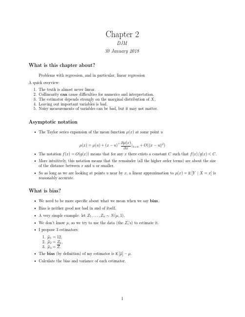
Chapter2DJM30January2018What is this chapter about?Problems with regression,and in particular,linear regressionA quick overview:1.The truth is almost never linear.2.Collinearity can cause difficulties for numerics and interpretation.3.The estimator depends strongly on the marginal distribution of X.4.Leaving out important variables is bad.5.Noisy measurements of variables can be bad,but it may not matter. Asymptotic notation•The Taylor series expansion of the mean functionµ(x)at some point uµ(x)=µ(u)+(x−u) ∂µ(x)∂x|x=u+O( x−u 2)•The notation f(x)=O(g(x))means that for any x there exists a constant C such that f(x)/g(x)<C.•More intuitively,this notation means that the remainder(all the higher order terms)are about the size of the distance between x and u or smaller.•So as long as we are looking at points u near by x,a linear approximation toµ(x)=E[Y|X=x]is reasonably accurate.What is bias?•We need to be more specific about what we mean when we say bias.•Bias is neither good nor bad in and of itself.•A very simple example:let Z1,...,Z n∼N(µ,1).•We don’t knowµ,so we try to use the data(the Z i’s)to estimate it.•I propose3estimators:1. µ1=12,2. µ2=Z6,3. µ3=Z.•The bias(by definition)of my estimator is E[ µ]−µ.•Calculate the bias and variance of each estimator.Regression in general•If I want to predict Y from X ,it is almost always the case thatµ(x )=E [Y |X =x ]=x β•There are always those errors O ( x −u )2,so the bias is not zero.•We can include as many predictors as we like,but this doesn’t change the fact that the world isnon-linear .Covariance between the prediction error and the predictors•In theory,we have (if we know things about the state of nature)β∗=arg min βE Y −Xβ 2 =Cov [X,X ]−1Cov [X,Y ]•Define v −1=Cov [X,X ]−1.•Using this optimal value β∗,what is Cov [Y −Xβ∗,X ]?Cov [Y −Xβ∗,X ]=Cov [Y,X ]−Cov [Xβ∗,X ](Cov is linear)=Cov [Y,X ]−Cov X (v −1Cov [X,Y ]),X(substitute the def.of β∗)=Cov [Y,X ]−Cov [X,X ]v −1Cov [X,Y ](Cov is linear in the first arg)=Cov [Y,X ]−Cov [X,Y ]=0.Bias and Collinearity•Adding or dropping variables may impact the bias of a model •Suppose µ(x )=β0+β1x 1.It is linear.What is our estimator of β0?•If we instead estimate the model y i =β0,our estimator of β0will be biased.How biased?•But now suppose that x 1=12always.Then we don’t need to include x 1in the model.Why not?•Form the matrix [1x 1].Are the columns collinear?What does this actually mean?When two variables are collinear,a few things happen.1.We cannot numerically calculate (X X )−1.It is rank deficient.2.We cannot intellectually separate the contributions of the two variables.3.We can (and should)drop one of them.This will not change the bias of our estimator,but it will alterour interpretations.4.Collinearity appears most frequently with many categorical variables.5.In these cases,software automatically drops one of the levels resulting in the baseline case being inthe intercept.Alternately,we could drop the intercept!6.High-dimensional problems (where we have more predictors than observations)also lead to rankdeficiencies.7.There are methods (regularizing)which attempt to handle this issue (both the numerics and theinterpretability).We may have time to cover them slightly.【原创】定制代写 r 语言/python/spss/matlab/WEKA/sas/sql/C++/stata/eviews 数据挖掘和统计分析可视化调研报告等服务(附代码数据),官网咨询链接:/teradat有问题到淘宝找“大数据部落”就可以了White noiseWhite noise is a stronger assumption than Gaussian .Consider a random vector .1. ∼N (0,Σ).2. i ∼N (0,σ2(x i )).3. ∼N (0,σ2I ).The third is white noise.The are normal,their variance is constant for all i and independent of x i ,and they are independent.Asymptotic efficiencyThis and MLE are covered in 420.There are many properties one can ask of estimators θof parameters θ1.Unbiased:E θ−θ=02.Consistent: θn →∞−−−−→θ3.Efficient:V θ is the smallest of all unbiased estimators4.Asymptotically efficient:Maybe not efficient for every n ,but in the limit,the variance is the smallest of all unbiased estimators.5.Minimax:over all possible estimators in some class,this one has the smallest MSE for the worst problem.6....Problems with R-squaredR 2=1−SSE ni =1(Y i −Y )2=1−MSE 1n n i =1(Y i −Y )2=1−SSE SST •This gets spit out by software •X and Y are both normal with (empirical)correlation r ,then R 2=r 2•In this nice case,it measures how tightly grouped the data are about the regression line •Data that are tightly grouped about the regression line can be predicted accurately by the regression line.•Unfortunately,the implication does not go both ways.•High R 2can be achieved in many ways,same with low R 2•You should just ignore it completely (and the adjusted version),and encourage your friends to do the sameHigh R-squared with non-linear relationshipgenY <-function (X,sig)Y =sqrt (X)+sig *rnorm (length (X))sig=0.05;n=100X1=runif (n,0,1)X2=runif (n,1,2)X3=runif (n,10,11)df =data.frame (x=c (X1,X2,X3),grp =rep (letters[1:3],each=n))df $y =genY (df $x,sig)ggplot (df,aes (x,y,color=grp))+geom_point ()+geom_smooth (method = lm ,fullrange=TRUE ,se =FALSE )+ylim (0,4)+stat_function (fun=sqrt,color= black)12340369xy grpab cdf %>%group_by (grp)%>%summarise (rsq =summary (lm (y ~x))$r.sq)###A tibble:3x 2##grp rsq ##<fctr><dbl>##1a 0.924##2b 0.845##3c 0.424。
