北大《自动控制原理》讲义 第三讲
- 格式:ppt
- 大小:917.00 KB
- 文档页数:47

第一章自动控制原理的基本概念主要内容:自动控制的基本知识开环控制与闭环控制自动控制系统的分类及组成自动控制理论的发展§1.1 引言控制观念生产和科学实践中,要求设备或装置或生产过程按照人们所期望的规律运行或工作。
同时,干扰使实际工作状态偏离所期望的状态。
例如:卫星运行轨道,导弹飞行轨道,加热炉出口温度,电机转速等控制控制:为了满足预期要求所进行的操作或调整的过程。
控制任务可由人工控制和自动控制来完成。
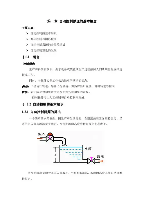
§ 1.2 自动控制的基本知识1.2.1 自动控制问题的提出一个简单的水箱液面,因生产和生活需要,希望液面高度h维持恒定。
当水的流入量与流出量平衡时,水箱的液面高度维持在预定的高度上。
当水的流出量增大或流入量减小,平衡则被破坏,液面的高度不能自然地维持恒定。
所谓控制就是强制性地改变某些物理量(如上例中的进水量),而使另外某些特定的物理量(如液面高度h)维持在某种特定的标准上。
人工控制的例子。
这种人为地强制性地改变进水量,而使液面高度维持恒定的过程,即是人工控制过程。
1.2.2 自动控制的定义及基本职能元件1. 自动控制的定义自动控制就是在没有人直接参与的情况下,利用控制器使被控对象(或过程)的某些物理量(或状态)自动地按预先给定的规律去运行。
当出水与进水的平衡被破坏时,水箱水位下降(或上升),出现偏差。
这偏差由浮子检测出来,自动控制器在偏差的作用下,控制阀门开大(或关小),对偏差进行修正,从而保持液面高度不变。
2. 自动控制的基本职能元件自动控制的实现,实际上是由自动控制装置来代替人的基本功能,从而实现自动控制的。
画出以上人工控制与动控制的功能方框图进行对照。
比较两图可以看出,自动控制实现人工控制的功能,存在必不可少的三种代替人的职能的基本元件:测量元件与变送器(代替眼睛)自动控制器(代替大脑)执行元件(代替肌肉、手)这些基本元件与被控对象相连接,一起构成一个自动控制系统。
下图是典型控制系统方框图。
![[工学]自动控制原理第3章](https://uimg.taocdn.com/d9a77406bf23482fb4daa58da0116c175f0e1e8a.webp)


Lecture3-Laplace TransformsK.J.ÅströmReview of control system analysis1.The Basic Feedback Loopplace T ransforms3.Analysis of Feedback Loops4.Qualitative Understanding of Signals and Systems5.SummaryTheme:Streamline manipulation of equations and block diagrams.Construction of a Block DiagramThe block diagram gives an overview.T o draw a block diagram:•Understand how the system works.•Identify the major components and the relevant signals.•Key questions:Where is the essential dynamics?What are appropriate abstractions?•Describe the dynamics of the blocks in terms of standard models.dt n+a1dn−1ydt n−1+...+b n u is characterized by two polynomialsA(s)=s n+a1s n−1+a2s n−2+...+a n−1s+a nB(s)=b1s n−1+b2s n−2+...+b n−1s+b n•The roots of A(s)are called poles of the system.•The roots of B(s)are called zeros of the system.•The transfer function of the system is G(s)=B(s)Linear Time Invariant Systems(LTI)d n ydt n−1+...+a n y=b1dn−1uInterpretation of the Impulse Responsey(t)=nk=1C k−1(t)eαk t+t(t−τ)u(τ)dτLet the system be initially at rest,i.e.C k=0and let the inputbe an impulse at time0.The output is theny(t)= (t)If the input is a unit step the output(the step response)isy(t)=t(t−τ)dτ=t(τ)dτExperimental determination of step and impulse responses.Recall Cruise ControlProcess modeldvdt2+(0.02+k)dedtThe mathematical tool of Laplace transforms is ideally suitedfor these type of calculations.An essential part of the languageof control.place TransformsConsider a function f defined on 0≤t <∞and a real number σ>0.Assume that f grows slower than e σt for large t .The Laplace transform F =L f of f is defined asL f =F (s )= ∞e −stf (t )dtExample 1:f (t )=1,F (s )=∞e −st dt =−1sExample 2:f (t )=e −at ,F (s )=∞e −(s +a )t dt =−1s +adt=∞e −stf (t )dt =e −st f (t )∞0+s∞e −stf (t )dt =−f (0)+s L fs)dv =f (0)Final value theoremlim s →0sF (s )=lim s →0∞0se −st f (t )dt =lims →0∞e −vf (vPropertiesLinearity:L (a f +b )=a L f +b L Differentiation:L dfs L fTime shift:L f (t −T )=e −sTL fTime stretch:L f (at )=1a ),a >0.Convolution:L t0f (t −τ) (τ)d τ=F (s )G (s )Final value Theorem †:lim s →0sF (s )=lim t →∞f (t )Initial value Theorem †:lim s →∞sF (s )=lim t →0f (t )•†:V alid only if limits exist!A (s )=B (s )s −α1+C 2s −αnC k =lim s →αk(s −αk )F (s )=B (αk )The time function corresponding to the transform isf (t )=C 1e α1t +C 2e α2t +...+C n e αn tParameters αk give shape and numbers C k give magnitudes.Notice that αk may be complex numbers.With multiple roots the constants C k are instead polynomials.Manipulating LTI Systems The differentiation property L dfCruise ControlProcess model:dvsE(s)Pure algebra gives relation between Laplace transforms of slopeΘreference V r and E by eliminating V and Us(s+0.02)+ks+k iE(s)=10sΘ(s)+s(s+0.02)V r(s)2+2ω0s+ω20Θ(s)=10θ0ω0te−ω0tω0te−ω0tThe largest error e max=10θ0e−1occurs for t=1/ωparegraph belowθ0=0.04ζ=1,ω0=0.05(dotted),ω0=0.1Discussion•What do we mean by a solution to a problem?•A historical perspectiveClosed form expressions,tables,curves •The role of computers•The necessity of insight and understanding•The need to check results•What properties can wefind easily using“back of an envelope”calculation.•A perspective on use of Laplace transforms in control engineering•A more general(biased personal)perspective.T echnology changes fast but engineering education changes slowly.U(s)=L yCar Model in Cruise Control Process modeldvU(s)=1U(s)=−10Transfer Function of PID ControllerThe error e is the input and the control signal u is the outputu=ke+k ite(τ))dτ+k ddeE(s)=k+k iTransfer Function of CarA simple model of a car on a horizontal road tells how its position y depends on the throttle.Let the mass be m and assume that the propelling force is proportional to the throttle wefindmd2yU(s)=kTransfer Function of Time DelayConsider a system where the output y is the input u delayed Ttime units.The input output relation isy(t)=u(t−T)and the transfer function isG(s)=Y(s)Transfer Function of Standard Model Consider the systemd n ydt n−1+...+a n y=b1dn−1us n+a1s n−1+a2s n−2+...+a n−1s+a nSolutionIntroduce Laplace transforms and transfer functions.We haveE =R − N +P (D +CE )Solving for E givesE =11+PCN −P5.Qualitative Understanding of Signals andSystemsTime responses can in principle be computed.T ables of Laplace transforms is a help but the work is quite tedious.Time responses are easy to compute using different types of software.•It is a good rule to always make order of magnitude calculations to make sure that results are reasonable whenever you use software.•Much insight can be obtained form very simple calcula-tions (series expansions and factorization).•Some results will be presented.•It will be discussed more in future lecturesA (s )=B (s )s −α1+C 2s −αnC k =lim s →αk(s −αk )F (s )=B (αk )Parameters αk (roots of A (s ))are easy to compute.The signal y (t )has the formy (t )=C 1e α1t +C 2e α2t +...+C n e αn tParameters αk give shape and C k give magnitudes.A (s )=s +5Example...For small s the Laplace transform is Y(s) 2.5/s,which implies that for large t the time function is y(t) 2.5.For larges we have Y(s) 1/s2.This means that for small t the time function isC(s)=s+5Insight from Transfer Functions•Derive transfer function G(s)=B(s)Insight from Transfer Functions•Make a series expansion of G(s)for small s(low fre-quency behavior,large t)G(s)=c−1s+c−2s k+...If c0=0like a static gain.If c−1=0and c−1=0like an integrator.If c−1=c−2=...=c−k+1=0and c k=0like k integrators.ExamplesE XAMPLE 1—PID CONTROLLERThe PID controller has the transfer functionG (s )=k +k is+k +k d sThis is already in series expansion form.For slow signals(small s )it behaves like an integrator and for fast signals (large s )it behaves like a differentiator.E XAMPLE 2—PID CONTROLLER WITHD ERIVATIVEF ILTERG (s )=k 1+11+s T d /NBehaves like a static gain k (1+N )for fast signals (large s ).。