常用概率分布函数

常见的几种分布函数概率论中，分布函数（distribution function）是描述随机变量取值的概率分布的函数。

常见的几种分布函数包括离散型分布函数、连续型分布函数以及混合分布函数。

1. 离散型分布函数离散型分布函数是指随机变量在有限或可数个点上取值的分布函数。

离散型分布函数的特点是其概率质量函数只在有限或可数个点上取值，或者说离散型分布函数所描述的随机变量的取值是离散的。

比较常见的离散型分布函数有：- 二项分布函数：二项分布函数是描述n个独立的、相同概率的随机试验中成功的次数的分布函数。

- 泊松分布函数：泊松分布函数是描述一定时间间隔内一个随机事件发生次数的分布函数。

- 几何分布函数：几何分布函数是描述进行一系列独立的、相同概率的实验，成功的次数需要进行多次才能得到的情况的分布函数。

2. 连续型分布函数连续型分布函数是指随机变量的取值范围为连续区间的分布函数。

连续型分布函数所描述的随机变量的取值是连续的。

比较常见的连续型分布函数有：- 正态分布函数：正态分布函数又称高斯分布函数，是一种描述随机变量分布最为常用的分布函数之一。

- 均匀分布函数：均匀分布函数是描述随机变量在一定区间内取值时等概率分布的分布函数。

- 指数分布函数：指数分布函数是描述随机变量取值时间间隔的分布函数。

3. 混合分布函数混合分布函数是指一个随机变量可以同时满足两种或两种以上的分布函数时的情况。

比较常见的混合分布函数有：- 混合正态分布函数：混合正态分布函数是指由多个正态分布函数混合而成的分布函数。

- 混合伯努利分布函数：混合伯努利分布函数是指由多个伯努利分布函数混合而成的分布函数。

总之，分布函数是描述随机变量的 one-stop-shop，而离散型、连续型和混合型都是这一目的下的不同实现方式。

不同的分布函数有不同的特点和应用场景，选择合适的分布函数是进行概率论研究和应用的前提。

目录1. 均匀分布 (1)2. 正态分布（高斯分布） (2)3. 指数分布 (2)4. Beta分布（：分布） (2)5. Gamm 分布 (3)6. 倒Gamm分布 (4)7. 威布尔分布（Weibull分布、韦伯分布、韦布尔分布） (5)8. Pareto 分布 (6)9. Cauchy分布（柯西分布、柯西-洛伦兹分布） (7)210. 分布（卡方分布） (7)8 11. t分布................................................9 12. F分布 ...............................................10 13. 二项分布............................................10 14. 泊松分布（Poisson 分布）.............................11 15. 对数正态分布........................................1. 均匀分布均匀分布X ~U（a,b）是无信息的，可作为无信息变量的先验分布。

2. 正态分布（高斯分布）当影响一个变量的因素众多，且影响微弱、都不占据主导地位时，这个变量 很可能服从正态分布，记作X~N （」f 2）。

正态分布为方差已知的正态分布N （*2）的参数」的共轭先验分布。

1 空f （x ）： —— e 2-J2 兀 o'E(X)， Var(X) _ c 23. 指数分布指数分布X ~Exp （ ）是指要等到一个随机事件发生，需要经历多久时间。

其 中，.0为尺度参数。

指数分布的无记忆性：Plx s t|X = P{X t}。

f （X ）二 y oiE(X) 一4. Beta 分布（一：分布）f （X ）二 E(X)Var(X)=(b-a)2 12Var(X)二1~2Beta 分布记为X 〜Be(a,b)，其中Beta(1,1)等于均匀分布，其概率密度函数 可凸也可凹。

常用的分布函数公式
常用的分布函数公式分布函数是概率论和统计学中重要的概念，用于描述随机变量的概率分布。

在实际应用中，我们经常需要使用一些常用的分布函数公式来计算概率或进行统计推断。

以下是一些常见的分布函数公式：1. 正态分布函数：正态分布是自然界中许多现象的模型，其分布函数可以用以下公式表示：
F(x) = 1/2 [1 + erf((x-μ)/(σ√2))] 其中，μ是正态分布的均值，σ是标准差，erf是误差函数。

2. 二项分布函数：二项分布是一种离散概率分布，用于描述在n次独立重复试验中成功次数的概率。

其分布函数可以用以下公式表示：
F(x) = Σ(i=0 to x) [C(n, i) * p^i * (1-p)^(n-i)] 其中，C(n, i)是组合数，p是每次试验成功的概率。

3. 泊松分布函数：泊松分布是一种离散概率分布，用于描述单位时间或空间内随机事件发生的次数。

其分布函数可以用以下公式表示：
F(x) = Σ(i=0 to x) [e^(-λ) * λ^i / i!] 其中，λ是单位时间或空间内随机事件的平均发生率。

4. t分布函数：t分布是用于小样本情况下进行统计推断的概率分布。

其分布函数可以用以
下公式表示：
F(x) = 1/2 + 1/2 * I(x/√(n-1), (n-1)/2, 1/2) 其中，n是样本容量，I是不完全贝塞尔函数。

以上是一些常用的分布函数公式，它们在概率论和统计学中具有广泛的应用。

通过了解和掌握这些公式，我们可以更好地理解和分析随机变量的概率分布，从而进行相应的统计推断和决策。

理解概率分布函数常见分布公式详解概率分布函数（Probability Distribution Function，简称PDF）是描述随机变量取值概率分布的函数，常用于统计学和概率论中。

在统计学中，常见的概率分布函数有众多的公式。

本文将详细解释几种常见的概率分布函数公式，包括均匀分布、正态分布、指数分布和泊松分布。

一、均匀分布均匀分布是最简单的概率分布函数之一，它在一个有限区间内的取值是均匀分布的。

均匀分布的概率密度函数公式为：f(x) = 1 / (b - a)，a ≤ x ≤ b其中，a和b分别是区间的上下界。

均匀分布的期望值（均值）为（a + b）/ 2，方差为（b - a）^2 / 12。

二、正态分布正态分布是自然界和社会现象中常见的概率分布函数。

它在统计学中有着重要的地位。

正态分布的概率密度函数（Probability Density Function，简称PDF）公式为：f(x) = (1 / (σ * √(2π))) * exp(-((x - μ)^2/(2σ^2)))其中，μ是期望值（均值），σ是标准差。

正态分布的期望值和方差分别为μ和σ^2。

三、指数分布指数分布是描述事件发生的时间间隔的概率分布函数，常用于可靠性工程和排队论中。

指数分布的概率密度函数公式为：f(x) = λ * exp(-λx)，x ≥ 0其中，λ是事件发生率。

指数分布的期望值为1 / λ，方差为1 / λ^2。

四、泊松分布泊松分布是描述单位时间或空间内事件发生次数的概率分布函数，常用于描述稀有事件的发生情况。

泊松分布的概率质量函数（Probability Mass Function，简称PMF）公式为：P(X = k) = (λ^k * exp(-λ)) / k!其中，λ是单位时间或空间内事件的平均发生率。

泊松分布的期望值和方差均为λ。

以上是几种常见的概率分布函数公式的详细解释。

这些概率分布函数在不同领域的应用非常广泛，能够描述和解释各种随机现象的概率分布情况。

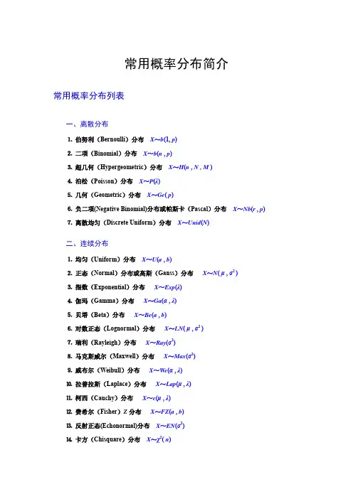
16种常见概率分布概率密度函数意义及其应用概率分布是统计学中一个重要的概念，用于描述随机变量在各个取值上的概率分布情况。

常见的概率分布有16种，它们分别是均匀分布、伯努利分布、二项分布、几何分布、泊松分布、正态分布、指数分布、负二项分布、超几何分布、Gumbel分布、Weibull分布、伽马分布、Beta分布、对数正态分布、卡方分布和三角分布。

以下将逐一介绍这些概率分布的概率密度函数、意义及其应用。

1. 均匀分布（Uniform Distribution）：概率密度函数为f(x)=1/(b-a)，意义是在一个区间内所有的取值具有相同的概率，应用有随机数生成、模拟实验等。

2. 伯努利分布（Bernoulli Distribution）：概率密度函数为P(x)=p^x*(1-p)^(1-x)，意义是在两种可能结果中，成功或失败的概率分布，应用有二分类问题的建模。

3. 二项分布（Binomial Distribution）：概率密度函数为P(x)=C(n,x)*p^x*(1-p)^(n-x)，意义是在n次独立重复试验中，成功次数为x的概率分布，应用有二分类问题中的n次重复试验。

4. 几何分布（Geometric Distribution）：概率密度函数为P(x)=p*(1-p)^(x-1)，意义是独立重复试验中，第x次成功所需的试验次数的概率分布，应用有描述一连串同样试验中第一次获得成功之前所需的试验次数。

5. 泊松分布（Poisson Distribution）：概率密度函数为P(x)=(e^(-λ)*λ^x)/x!，意义是在给定时间或空间内事件发生的次数的概率分布，应用有描述单位时间或单位空间内的事件计数问题。

6. 正态分布（Normal Distribution）：概率密度函数为P(x) = (1 / sqrt(2πσ^2)) * e^(-(x-μ)^2 / (2σ^2))，意义是描述连续变量的概率分布，应用广泛，例如测量误差、人口身高等。

概率论分布函数概率论分布函数是概率论中的重要概念，它描述了一个随机变量取值的概率分布情况。

在统计学和概率论中，有许多常见的概率分布函数，如正态分布、均匀分布、泊松分布等。

本文将针对这些常见的概率分布函数进行介绍和解释。

一、正态分布（Normal Distribution）正态分布是自然界中最常见的分布之一。

它以钟形曲线形式展现，其分布函数描述了随机变量在不同取值上的概率密度。

正态分布的特点是对称且呈现出标准差的影响，标准差越大，曲线越平缓。

正态分布广泛应用于自然科学、社会科学等领域，用于描述各种现象的分布情况。

二、均匀分布（Uniform Distribution）均匀分布是最简单的概率分布之一，它描述了随机变量在一定范围内各个取值出现的概率是相等的。

均匀分布的分布函数是一个常数函数，其特点是在一定范围内的取值概率是相等的。

均匀分布常用于模拟随机事件或生成随机数，广泛应用于数值计算和概率统计等领域。

三、泊松分布（Poisson Distribution）泊松分布是用于描述单位时间（或空间）内随机事件发生次数的概率分布。

泊松分布的分布函数可以表示在一段时间或空间内发生某种事件的次数的概率。

泊松分布的特点是具有独立性和稀有性，适用于描述稀有事件的发生情况，如电话交换机接听电话的次数、汽车在某路段通过的次数等。

四、指数分布（Exponential Distribution）指数分布是一种连续概率分布函数，描述了随机事件发生的时间间隔的概率分布。

指数分布的分布函数具有单峰性，随着时间的推移，事件发生的概率逐渐减小。

指数分布常用于描述随机事件的间隔时间，如人们等待公交车的时间、网络传输数据包到达的时间等。

五、二项分布（Binomial Distribution）二项分布是描述在一次试验中成功次数的概率分布函数。

二项分布的分布函数描述了在一定次数的独立重复试验中成功次数的概率分布情况。

二项分布的特点是具有两个参数，成功概率和试验次数，常用于描述二元随机事件的发生情况，如硬币正反面的次数、投篮命中的次数等。

Diagram of distribution relationships Probability distributions have a surprising number inter-connections. A dashed line in the chart below indicates an approximate (limit) relationship between two distribution families. A solid line indicates an exact relationship: special case, sum, or transformation.Click on a distribution for the parameterization of that distribution. Click on an arrow for details on the relationship represented by the arrow. Other diagrams on this site:The chart above is adapted from the chart originally published by Lawrence Leemis in 1986 (Relationships Among Common Univariate Distributions, American Statistician 40:143-146.) Leemis published a larger chart in 2008 which is available online.The precise relationships between distributions depend on parameterization. The relationships detailed below depend on the following parameterizations for the PDFs.Let C(n, k) denote the binomial coefficient(n, k) and B(a, b) = Γ(a) Γ(b) / Γ(a + b).Geometric: f(x) = p (1-p)x for non-negative integers x.Discrete uniform: f(x) = 1/n for x = 1, 2, ..., n.Negative binomial: f(x) = C(r + x - 1, x) p r(1-p)x for non-negative integers x. See notes on the negative binomial distribution.Beta binomial: f(x) = C(n, x) B(α + x, n + β - x) / B(α, β) for x = 0, 1, ..., n. Hypergeometric: f(x) = C(M, x) C(N-M, K - x) / C(N, K) for x = 0, 1, ..., N. Poisson: f(x) = exp(-λ) λx/ x! for non-negative integers x. The parameter λ is both the mean and the variance.Binomial: f(x) = C(n, x) p x(1 - p)n-x for x = 0, 1, ..., n.Bernoulli: f(x) = p x(1 - p)1-x where x = 0 or 1.Lognormal: f(x) = (2πσ2)-1/2 exp( -(log(x) - μ)2/ 2σ2) / x for positive x. Note that μ and σ2are not the mean and variance of the distribution.Normal : f(x) = (2π σ2)-1/2 exp( - ½((x - μ)/σ)2 ) for all x.Beta: f(x) = Γ(α + β) xα-1(1 - x)β-1/ (Γ(α) Γ(β)) for 0 ≤ x ≤ 1.Standard normal: f(x) = (2π)-1/2 exp( -x2/2) for all x.Chi-squared: f(x) = x-ν/2-1 exp(-x/2) / Γ(ν/2) 2ν/2for positive x. The parameter ν is called the degrees of freedom.Gamma: f(x) = β-α xα-1 exp(-x/β) / Γ(α) for positive x. The parameter α is called the shape and β is the scal e.Uniform: f(x) = 1 for 0 ≤ x ≤ 1.Cauchy: f(x) = σ/(π( (x - μ)2+ σ2) ) for all x. Note that μ and σ are location and scale parameters. The Cauchy distribution has no mean or variance. Snedecor F: f(x) is proportional to x(ν1 - 2)/2/ (1 + (ν1/ν2) x)(ν1 + ν2)/2 for positive x. Exponential: f(x) = exp(-x/μ)/μ for positive x. The parameter μ is the mean.Student t: f(x) is proportional to (1 + (x2/ν))-(ν + 1)/2 for positive x. The parameter ν is called the degrees of freedom.Weibull: f(x) = (γ/β) xγ-1 exp(- xγ/β) for positive x. The parameter γ is the shape and β is the scale.Double exponential : f(x) = exp(-|x-μ|/σ) / 2σ for all x. The parameter μ is the location and mean; σ is the scale.For comparison, see distribution parameterizations in R/S-PLUS and Mathematica.In all statements about two random variables, the random variables are implicitly independent.Geometric / negative binomial: If each X i is geometric random variable with probability of success p then the sum of n X i's is a negative binomial random variable with parameters n and p.Negative binomial / geometric: A negative binomial distribution with r = 1 is a geometric distribution.Negative binomial / Poisson: If X has a negative binomial random variable with r large, p near 1, and r(1-p) = λ, then F X≈ F Y where Y is a Poisson random variable with mean λ.Beta-binomial / discrete uniform: A beta-binomial (n, 1, 1) random variable is a discrete uniform random variable over the values 0 ... n.Beta-binomial / binomial: Let X be a beta-binomial random variable with parameters (n, α, β). Let p = α/(α + β) and suppose α + β is large. If Y is a binomial(n, p) random variable then F X≈ F Y.Hypergeometric / binomial: The difference between a hypergeometric distribution and a binomial distribution is the difference between sampling without replacement and sampling with replacement. As the population size increases relative to the sample size, the difference becomes negligible. Geometric / geometric: If X1 and X2 are geometric random variables with probability of success p1 and p2 respectively, then min(X1, X2) is a geometric random variable with probability of success p = p1 + p2 - p1 p2. The relationship is simpler in terms of failure probabilities: q = q1 q2.Poisson / Poisson: If X1 and X2are Poisson random variables with means μ1 and μ2respectively, then X1 + X2is a Poisson random variable with mean μ1 + μ2.Binomial / Poisson: If X is a binomial(n, p) random variable and Y is a Poisson(np) distribution then P(X = n) ≈ P(Y = n) if n is large and np is small. For more information, see Poisson approximation to binomial.Binomial / Bernoulli: If X is a binomial(n, p) random variable with n = 1, X is a Bernoulli(p) random variable.Bernoulli / Binomial: The sum of n Bernoulli(p) random variables is a binomial(n, p) random variable.Poisson / normal: If X is a Poisson random variable with large mean and Y is a normal distribution with the same mean and variance as X, then for integers j and k, P(j ≤ X ≤ k) ≈ P(j - 1/2 ≤ Y ≤ k + 1/2). For more information, see normal approximation to Poisson.Binomial / normal: If X is a binomial(n, p) random variable and Y is a normal random variable with the same mean and variance as X, i.e. np and np(1-p), then for integers j and k, P(j ≤ X ≤ k) ≈ P(j - 1/2 ≤ Y ≤ k + 1/2). Theapproximation is better when p ≈ 0.5 and when n is large. For more information, see normal approximation to binomial.Lognormal / lognormal: If X1 and X2 are lognormal random variables with parameters (μ1, σ12) and (μ2, σ22) respectively, then X1 X2 is a lognormal random variable with parameters (μ1+ μ2, σ12+ σ22).Normal / lognormal: If X is a normal (μ, σ2) random variable then e X is a lognormal (μ, σ2) random variable. Conversely, if X is a lognormal (μ, σ2) random variable then log X is a normal (μ, σ2) random variable.Beta / normal: If X is a beta random varia ble with parameters α and β equal and large, F X≈ F Y where Y is a normal random variable with the same mean and variance as X, i.e. mean α/(α + β) and variance αβ/((α+β)2(α + β + 1)). For more information, see normal approximation to beta.Normal / standard normal: If X is a normal(μ, σ2) random variable then (X - μ)/σ is a standard normal random variable. Conversely, If X is a normal(0,1) random variable then σ X + μ is a normal (μ, σ2) random variable.Normal / normal: If X1is a normal (μ1, σ12) random variable and X2 is a normal (μ2, σ22) random variable, then X1 + X2is a normal (μ1+ μ2, σ12+ σ22) random variable.Gamma / normal: If X is a gamma(α, β) random variable and Y is a normal random variable with the same mean and variance as X, then F X≈ F Y if the shape parameter α is large relative to the scale parameter β. For more information, see normal approximation to gamma.Gamma / beta: If X1 is gamma(α1, 1) random variable and X2is a gamma (α2, 1) random variable then X1/(X1 + X2) is a beta(α1, α2) random variable. More generally, if X1is gamma(α1, β1) random variable and X2is gamma(α2, β2) random variable then β2 X1/(β2 X1+ β1 X2) is a beta(α1, α2) random variable. Beta / uniform: A beta random variable with parameters α = β = 1 is a uniform random variable.Chi-squared / chi-squared: If X1 and X2 are chi-squared random variables with ν1and ν2 degrees of freedom respectively, then X1 + X2 is a chi-squared random variable with ν1+ ν2 degrees of freedom.Standard normal / chi-squared: The square of a standard normal random variable has a chi-squared distribution with one degree of freedom. The sum of the squares of n standard normal random variables is has a chi-squared distribution with n degrees of freedom.Gamma / chi-squared: If X is a gamma (α, β) random variable with α = ν/2 and β = 2, then X is a chi-squared random variable with ν degrees of freedom. Cauchy / standard normal: If X and Y are standard normal random variables, X/Y is a Cauchy(0,1) random variable.Student t / standard normal: If X is a t random variable with a large number of degrees of freedom ν then F X≈ F Y where Y is a standard normal random variable. For more information, see normal approximation to t.Snedecor F / chi-squared: If X is an F(ν, ω) random variable with ω large, then ν X is approximately distributed as a chi-squared random variable with ν degrees of freedom.Chi-squared / Snedecor F: If X1 and X2 are chi-squared random variables with ν1and ν2 degrees of freedom respectively, then (X1/ν1)/(X2/ν2) is an F(ν1, ν2) random variable.Chi-squared / exponential: A chi-squared distribution with 2 degrees of freedom is an exponential distribution with mean 2.Exponential / chi-squared: An exponential random variable with mean 2 is a chi-squared random variable with two degrees of freedom.Gamma / exponential: The sum of n exponential(β) random variables is a gamma(n, β) rand om variable.Exponential / gamma: A gamma distribution with shape parameter α = 1 and scale parameter β is an exponential(β) distribution.Exponential / uniform: If X is an exponential random variable with mean λ, then exp(-X/λ) is a uniform random variabl e. More generally, sticking any random variable into its CDF yields a uniform random variable.Uniform / exponential: If X is a uniform random variable, -λ log X is an exponential random variable with mean λ. More generally, applying the inverse CDF of any random variable X to a uniform random variable creates a variable with the same distribution as X.Cauchy reciprocal: If X is a Cauchy (μ, σ) random variable, then 1/X is a Cauchy (μ/c, σ/c) random variable where c = μ2+ σ2.Cauchy sum: If X1 is a Cauchy (μ1, σ1) random variable and X2 is a Cauchy (μ2, σ2), then X1 + X2is a Cauchy (μ1+ μ2, σ1+ σ2) random variable. Student t / Cauchy: A random variable with a t distribution with one degree of freedom is a Cauchy(0,1) random variable.Student t / Snedecor F: If X is a t random variable with ν degree of freedom, then X2is an F(1,ν) random variable.Snedecor F / Snedecor F: If X is an F(ν1, ν2) random variable then 1/X is an F(ν2, ν1) random variable.Exponential / Exponential: If X1 and X2 are exponential random variables with mean μ1and μ2 respectively, then min(X1, X2) is an exponential random variable with mean μ1μ2/(μ1+ μ2).Exponential / Weibull: If X is an exponential random variable with mean β, then X1/γis a Weibull(γ, β) random variable.Weibull / Exponential: If X is a Weibull(1, β) random variable, X is an exponential random variable with mean β.Exponential / Double exponential: If X and Y are exponential random variables with mean μ, then X-Y is a double exponential random variable with mean 0 and scale μDouble exponential / exponential: If X is a double exponential random variable with mean 0 and scale λ, then |X| is an exponential random variable with mean λ.。

概率分布函数的常用公式整理概率分布函数是描述随机变量在不同取值下的概率分布的函数，是统计学中重要的概念。

在实际应用中，我们常常需要计算或查阅各种概率分布函数的公式，以便进行数据分析和决策。

下面是一些常用的概率分布函数和相关公式的整理。

1. 二项分布（Binomial Distribution）二项分布是一种离散型概率分布，描述了在n次独立实验中成功次数的概率分布。

二项分布的概率质量函数（Probability Mass Function, PMF）和累积分布函数（Cumulative Distribution Function, CDF）分别为：PMF: P(X = k) = C(n, k) * p^k * (1-p)^(n-k)CDF: P(X ≤ k) = Σ(C(n, i) * p^i * (1-p)^(n-i)), 0 ≤ i ≤ k其中，X表示成功次数，k表示取值，n表示实验次数，p表示单次实验的成功概率，C(n, k)表示组合数。

2. 泊松分布（Poisson Distribution）泊松分布是一种描述单位时间或空间内随机事件发生次数的概率分布。

泊松分布的概率质量函数和累积分布函数为：PMF: P(X = k) = (λ^k * e^(-λ)) / k!CDF: P(X ≤ k) = Σ(λ^i * e^(-λ)) / i!, 0 ≤ i ≤ k其中，X表示事件发生次数，k表示取值，λ表示事件发生的平均次数。

3. 正态分布（Normal Distribution）正态分布是一种连续型概率分布，以钟形曲线来描述数据分布。

正态分布的概率密度函数（Probability Density Function, PDF）和累积分布函数为：PDF: f(x) = (1 / (σ * √(2π))) * e^(-(x-μ)^2 / (2σ^2))CDF: P(X ≤ x) = (1 / 2) * (1 + erf((x-μ) / (σ√2)))其中，X表示随机变量取值，μ表示均值，σ表示标准差，π表示圆周率，erf表示高斯误差函数。

八大分布函数表在学习统计学时，概率函数是我们必须掌握的重要概念。

它用于表示一个随机变量的概率分布情况，比如说我们可以得到一个随机变量的期望值或者方差等信息，而这些都是基于概率函数的。

概率函数有很多种，其中最常用的就是八大分布函数表。

八大分布函数表是概率分布函数的最重要的表示形式。

它们之所以被称为“八大”，是因为它们包含概率分布函数中最常见的八种函数。

它们分别为：正态分布函数，卡方分布函数，指数分布函数，Beta 分布函数，泊松分布函数，F分布函数，t分布函数和τ函数。

它们的具体的表达形式如下：1.态分布函数：f(x) = 1/(σ√2π) * e^-(x-μ)^2/2σ^22.方分布函数：f(x) = 1/(2^(k/2) (k/2))x^(k/2-1)e^-x/23.数分布函数：f(x) =e^-λx4. Beta分布函数：f(x) = (α +) / (α) (β) x^(α - 1) (1 - x)^(β - 1) 5.松分布函数：f(x) =^x / x! e^-λ6. F分布函数：f(x) = (Γ ((m+n)/2)/Γ (m/2)Γ (n/2)) (m/n)^(m/2)x^((m-2)/2) (1+m/nx)^(-(m+n)/2)7. t分布函数：f(x) = ( (ν+1) / 2) / (π^(1/2) (ν /2)) (1 + (x^2 /))^(- (ν +1) /2)8.函数：f(x) = (1/(π))^(1/2) (1 + (x/ν))^(-1/2)以上就是八大分布函数表的定义。

虽然它们的表达形式有所不同，但它们的特征都是由参数，σ，λ，α，β，k，ν决定的。

在统计学中，八大分布函数表被广泛应用。

它们可以用来描述一组样本数据的概率分布情况，也可以用来估算样本数据的期望值或样本方差等概率特性。

此外，八大分布函数表还可以用来建立多项式拟合模型，用来描述和估算离散变量的变化趋势。

概率分布函数概率分布函数（Probability Distribution Function）是在概率论与数理统计中用来描述随机变量的分布规律的函数。

它可以提供随机变量取某个值的概率。

一、定义与性质概率分布函数通常表示为 F(x)，其中 x 是随机变量的取值，F(x) 表示该变量小于等于 x 的概率。

概率分布函数具有以下性质：1. 非减性：随着 x 增大，F(x) 逐渐增大或保持不变。

2. 有界性：0 ≤ F(x) ≤ 1，对于任意的 x。

3. 右连续性：在所有的实数 x0，F(x) 在 x ≥ x0 时连续。

二、常见1. 均匀分布函数（Uniform Distribution Function）：均匀分布函数是一种简单且常见的概率分布函数。

在一个区间 [a, b] 内，每个数值的概率密度相等，即 f(x) = 1 / (b - a)，其中a ≤ x ≤ b。

其概率分布函数为：F(x) = (x - a) / (b - a)，其中a ≤ x ≤ b。

2. 正态分布函数（Normal Distribution Function）：正态分布函数也被称为高斯分布函数。

它是一种常见的连续概率分布函数，通常用于描述自然界中的现象。

其概率密度函数为：f(x) = (1 / (σ * √(2π))) * exp(-(x - μ)² / (2 * σ²))，其中μ 是均值，σ 是标准差。

其概率分布函数无法用简单的公式表示，常用统计软件进行计算。

3. 二项分布函数（Binomial Distribution Function）：二项分布函数用于描述在 n 个独立的 Bernoulli 试验中成功的次数的概率分布。

其中成功的概率为 p，失败的概率为 q = 1 - p。

其概率质量函数为：f(x) = C(n, x) * p^x * q^(n-x)，其中 C(n, x) 表示组合数。

其概率分布函数通常写为累积形式，无法用简单的公式表示。

常见的分布函数常见的分布函数包括：1. 正态分布函数（Normal Distribution Function）：也称为高斯分布函数，是最常见的概率分布函数之一，用于描述一组数据在平均值附近的分布情况。

其概率密度函数为：$$f(x)=\frac{1}{\sqrt{2\pi}\sigma}e^{-\frac{(x-\mu)^2}{2\sigma^2}}$$。

2. 均匀分布函数（Uniform Distribution Function）：是一种简单的概率分布函数，表示在一个区间内随机抽取数据的均匀分布情况。

其概率密度函数为：$$f(x)=\begin{cases}。

\frac{1}{b-a} & a\leq x \leq b \\。

0 & \text{其他}。

\end{cases}$$。

3. 伽马分布函数（Gamma Distribution Function）：适用于描述正值的数据分布情况，常用于计算无线电信号的强度、生物统计学等领域。

其概率密度函数为：$$f(x)=\frac{1}{\Gamma(\alpha)\beta^\alpha}x^{\alpha-1}e^{-\frac{x}{\beta}}$$。

4. 指数分布函数（Exponential Distribution Function）：是一种描述随机事件发生时间间隔的概率分布函数，常用于生物学、金融等领域。

其概率密度函数为：$$f(x)=\begin{cases}。

\lambda e^{-\lambda x} & x \geq 0 \\。

0&x<0。

\end{cases}$$。

5. 泊松分布函数（Poisson Distribution Function）：用于描述事件的随机发生次数，常用于工业、生物学等领域。

其概率密度函数为：$$f(x)=\frac{\lambda^x}{x!}e^{-\lambda}$$。

概率论八大分布公式概率论中的八大分布公式是指常见的概率分布函数，它们在统计学和概率分析中有着广泛的应用。

这些分布包括：二项分布、泊松分布、均匀分布、正态分布、指数分布、伽玛分布、贝塔分布和卡方分布。

下面将对这八个分布公式进行简要介绍。

1. 二项分布二项分布是离散概率分布的一种，适用于只有两种可能结果的事件，如投掷硬币的结果。

它的概率分布函数可以用来计算在n次独立重复试验中，成功事件发生k次的概率。

2. 泊松分布泊松分布是一种离散概率分布，用于描述单位时间或空间内事件发生的次数。

它的概率分布函数可以用来计算在一个固定时间或空间单位内，事件发生k次的概率。

3. 均匀分布均匀分布是一种连续概率分布，它的概率密度函数在一个区间内的取值相等。

例如，投掷一个均匀骰子的结果就符合均匀分布。

4. 正态分布正态分布是一种连续概率分布，也被称为高斯分布。

它的概率密度函数呈钟形曲线，对称分布在均值附近。

许多自然界的现象都可以用正态分布来描述，如身高、体重等。

5. 指数分布指数分布是一种连续概率分布，用于描述事件发生的间隔时间。

它的概率密度函数呈指数下降的形式，适用于模拟一些随机事件的发生。

6. 伽玛分布伽玛分布是一种连续概率分布，它的概率密度函数呈正偏态分布。

伽玛分布常用于描述一些随机变量的持续时间，如寿命、等待时间等。

7. 贝塔分布贝塔分布是一种连续概率分布，它的概率密度函数呈S形曲线。

贝塔分布常用于描述概率或比率的分布，如投掷硬币的概率、产品的可靠性等。

8. 卡方分布卡方分布是一种连续概率分布，它的概率密度函数呈非对称形状。

卡方分布常用于统计推断中的假设检验和置信区间估计，如样本方差的分布。

概率论八大分布公式涵盖了离散分布和连续分布的常见情况。

这些分布公式在实际应用中具有重要的意义，可用于模拟随机事件、进行统计推断以及进行风险评估等。

熟练掌握这些分布公式，对于数据分析和决策制定都具有重要的帮助。

常见分布的概率密度函数在概率统计学中，常见分布的概率密度函数是非常重要的一部分。

它们被广泛地应用于各种领域，如工程、医学和金融学等。

在本文中，我们将讨论几个常见的概率密度函数以及它们的特点。

一、正态分布正态分布是一种非常重要的分布，因为它在自然界和社会科学中出现的频率非常高。

正态分布的概率密度函数可以用以下公式表示：$f(x)=\frac{1}{\sigma \sqrt{2\pi}}e^{-\frac{(x-\mu)^2}{2\sigma^2}}$其中，$\mu$是正态分布的平均值，$\sigma$是标准差。

正态分布具有对称性，即左右两侧的概率密度相等。

此外，它的均值、中位数和众数均相等。

二、指数分布指数分布是描述等待时间的分布，它的概率密度函数可以用以下公式表示：$f(x)=\lambda e^{-\lambda x}$其中，$\lambda$是指数分布的参数，表示等待时间的平均值。

指数分布具有无记忆性，即它的概率密度不受过去等待时间的影响。

三、t分布t分布是应用到小样本情况下的一种分布，它较正态分布更为宽平，有更多的尾部。

t分布的概率密度函数可以用以下公式表示：$f(x)=\frac{\Gamma(\frac{\nu+1}{2})}{\sqrt{\nu\pi}\Gamma(\frac{\nu}{2})}(1+\frac{x^2}{\nu})^{-\frac{\nu+1}{2}}$其中，$\nu$是t分布的自由度，它决定了t分布的形状。

当自由度越大时，t分布趋向于正态分布。

四、卡方分布卡方分布是应用到两个或多个正态分布之和的分布，它也是一种重要的分布。

卡方分布的概率密度函数可以用以下公式表示：$f(x)=\frac{1}{\Gamma(\frac{\nu}{2})2^{\frac{\nu}{2}}}\c dot x^{\frac{\nu}{2}-1}e^{-\frac{x}{2}}$其中，$\nu$是卡方分布的自由度，它决定了卡方分布的形状。

概率数学分布函数归纳总结概率数学中的分布函数是指描述随机变量取值的概率分布的函数。

在概率论和统计学中，有许多常见的分布函数，它们都有各自的特点和应用领域。

在这篇文章中，我将对一些常见的分布函数进行归纳总结。

1.二项分布：二项分布是一种离散型的概率分布，描述了在一系列独立的、重复的伯努利试验中成功的次数。

它的概率质量函数为：P(X=k)=C(n,k)*p^k*(1-p)^(n-k)，其中n表示试验的次数，k表示成功的次数，p表示每次试验成功的概率。

2.泊松分布：泊松分布是一种离散型的概率分布，描述了在一段时间或一定空间内随机事件发生的次数。

它的概率质量函数为：P(X=k)=(λ^k*e^(-λ))/k!，其中λ表示在单位时间或单位空间内平均发生的事件次数。

3. 正态分布：正态分布是一种连续型的概率分布，也被称为高斯分布。

它是概率理论中最重要的分布之一，具有广泛的应用。

正态分布由均值μ和方差σ^2完全描述，其概率密度函数为：f(x) = (1 / (σ * sqrt(2 * π))) * e^((-(x-μ)^2) / (2 * σ^2))。

4.均匀分布：均匀分布是一种连续型的概率分布，在一些区间内的取值概率是相等的。

它的概率密度函数为：f(x)=1/(b-a)，其中a和b分别为区间的下界和上界。

5.指数分布：指数分布是一种连续型的概率分布，经常用于描述连续事件之间的时间间隔。

它的概率密度函数为：f(x)=λ*e^(-λx)，其中λ为事件发生的速率参数。

6.γ分布：γ分布是一种连续型的概率分布，常用于描述连续变量的正值分布。

γ分布是指数分布的推广，它的概率密度函数为：f(x)=(1/(Γ(α)*β^α))*x^(α-1)*e^(-x/β)，其中α和β为分布的形状参数。

7.β分布：β分布是一种连续型的概率分布，常用于表示随机事件概率的不确定性。

它的概率密度函数为：f(x)=(1/(β(α,β)))*x^(α-1)*(1-x)^(β-1)，其中α和β为分布的形状参数。