CFD modelling of bubble–particle attachments in flotation cells

PLEASE SCROLL DOWN FOR ARTICLEThis article was downloaded by: [Shanghai Jiaotong University]On: 15 September 2009Access details: Access Details: [subscription number 912295284]Publisher Taylor & FrancisInforma Ltd Registered in England and Wales Registered Number: 1072954 Registered office: Mortimer House,37-41 Mortimer Street, London W1T 3JH, UKInternational Journal of Computational Fluid DynamicsPublication details, including instructions for authors and subscription information:/smpp/title~content=t713455064Hydrodynamic modelling and CFD simulation of ferrofluids flow in magnetic targeting drug deliveryShigang Wang a ; Handan Liu a ; Wei Xu a aSchool of Mechanical Engineering, Shanghai Jiaotong University, Shanghai, China Online Publication Date: 01 December 2008To cite this Article Wang, Shigang, Liu, Handan and Xu, Wei(2008)'Hydrodynamic modelling and CFD simulation of ferrofluids flow inmagnetic targeting drug delivery',International Journal of Computational Fluid Dynamics,22:10,659 — 667To link to this Article: DOI: 10.1080/10618560802452009URL: /10.1080/10618560802452009Full terms and conditions of use: /terms-and-conditions-of-access.pdf This article may be used for research, teaching and private study purposes. Any substantial or systematic reproduction, re-distribution, re-selling, loan or sub-licensing, systematic supply or distribution in any form to anyone is expressly forbidden.The publisher does not give any warranty express or implied or make any representation that the contents will be complete or accurate or up to date. The accuracy of any instructions, formulae and drug doses should be independently verified with primary sources. The publisher shall not be liable for any loss,actions, claims, proceedings, demand or costs or damages whatsoever or howsoever caused arising directly or indirectly in connection with or arising out of the use of this material.Hydrodynamic modelling and CFD simulation of ferrofluids flow in magnetic targeting drugdeliveryShigang Wang,Handan Liu*and Wei XuSchool of Mechanical Engineering,Shanghai Jiaotong University,Shanghai 200240,China(Received 25January 2008;final version received 4October 2008)Magnetic targeting drug delivery is a method of carrying drug-loaded magnetic nanoparticles to a tissue target in the human body under the applied magnetic field.This method increases the drug concentration in the target and reduces the adverse side-effects.In this article,a mathematical model is presented to describe the hydrodynamics of ferrofluids as drug carriers flowing in a blood vessel under the applied magnetic field.Numerical simulations are performed to obtain better insight into the theoretical analysis with computational fluid dynamics.A 3D flow field of magnetic particles in an idealised blood vessel model containing an aneurysm is analysed to further understand clinical application of magnetic targeting drug delivery.Simulation samples demonstrate the important parameters leading to adequate drug delivery to the target site depending on the applied magnetic field in coincidence with reported results from animal experiments.Results of the analysis provide the important information and can suggest strategies for improving delivery in favour of the clinical application.Keywords:magnetic targeting drug delivery;ferrofluids;magnetic nanoparticles;hydrodynamic modelling;CFD simulation1.IntroductionIn conventional drug delivery the drug is administered by intravenous injection;it then travels to the heart from where it is pumped to all regions of the body.For the small target region that the drug is aimed at,this method is extremely inefficient and leads to much larger doses (often of toxic drugs)than necessary.To overcome this problem,a number of targeted drug delivery methods have been developed (Torchilin 2000,Lu bbe et al.2001,Vasir and Labhasetwar 2005).Among them,the mag-netic targeted drug delivery system is one of the most attractive strategies because of its non-invasiveness,high targeting efficiency and its ability to minimise the toxic side effects on healthy cells and tissues (Alexiou et al.2000,2005).Magnetic drug targeting therapy is a promising technique for the treatment of various diseases,especially cancer,arteriosclerosis,like stenosis,thrombosis and aneurysm,what is important is to keep the therapeutic drug in the targeting site,which is located along the inner wall of the blood vessel (Alksne et al.1967,Alexiou et al.2000,2005,Chen et al.2005,Udrea et al.2006).Some in vitro (Chen et al.2005,Udrea et al.2006)and in vivo (Alksne et al.1967,Goodwin et al.1999,Alexiou et al.2002,Jurgons et al.2006)experi-ments have been performed in this direction.Typically,this compound in which drugs are bound with nanoparticles is injected through a blood vesselsupplying the targeting tissue in the presence of an external magnetic field with sufficient field strength and gradient to retain the carrier at the target site.Recent development on carriers has largely focused on new polymeric or inorganic coatings on magnetite/maghemite nanoparticles (Ruuge and Rusetski 1993),such as ferrofluids.Ferrofluids are colloidal solutions of ferro or ferromagnetic nanoparticles in a carrier fluid,which are widely used in technical applications.Because of a high magnetic moment of nanoparticles in ferrofluids,ferrofluids are gaining increasing interest to be utilised as drug carriers in magnetic targeting for biological and medical applications (Riviere et al.2006).When they are used in medicine,ferrofluids must be bio-compatible and bio-degradable (Jurgons et al.2006).Recently,some theoretical studies of magnetically targeted drug delivery considered tracking individual particles under the influence of Stokes drag and a magnetic force alone (Grief and Richardson 2005),and formulated a two-dimensional (2D)model,suitable for studying the deposition of magnetic particles within a network of blood vessels (Richardson et al.2000).Other theoretical studies investigated the basic inter-action between magnetic and fluid shear forces in a blood vessel (Voltairas et al.2002)or utilised high gradient magnetic separation principles to study a*Corresponding author.Email:helenlew818@International Journal of Computational Fluid Dynamics Vol.22,No.10,December 2008,659–667ISSN 1061-8562print/ISSN 1029-0257online Ó2008Taylor &FrancisDOI:10.1080/10618560802452009D o w n l o a d e d B y : [S h a n g h a i J i a o t o n g U n i v e r s i t y ] A t : 16:26 15 S e p t e m b e r 2009magnetic drug targeting system(Ritter et al.2004). Although there have been a number of theoretical studies for magnetic drug targeting,very few research-ers have addressed the hydrodynamic models of magneticfluids in magnetic drug targeting delivery. Thus,the transport issues related to magnetic drug targeting delivery are yet poorly understood and it retards the extensive application of the magnetic drug targeting delivery.Therefore,it is very necessary to study theflow of the ferrofluids in the blood vessel under the action of the external magneticfield.In this article,we focused on investigating theflow rules of ferrofluids as drug carriers under the applied magneticfield.A mathematical model presented in this article describes the hydrodynamics of ferrofluids in a blood vessel under the action of the magneticfield. Numerical simulations are performed to obtain better insight into the theoretical analysis.Furthermore,the ferrofluidsflow is analysed numerically with com-putationalfluid dynamics(CFD)in a model of an idealised3D blood vessel containing an aneurysm to understand the clinical application of ferrofluids. Magneticfluids have been used in medicine since1960 for,e.g.the magnetically controlled metallic thrombosis of intracranial aneurysms(Alksne et al.1967).The biokinetic behaviour of ferrofluids in vivo was investi-gated and showed that the retention of ferrofluids in target region is dependent on the magneticfield strength(Goodwin et al.1999,Alexiou et al.2002, Jurgons et al.2006).Results of the analysis provided important information leading to adequate drug deliv-ery to the target site and can suggest strategies for improving delivery in favour of the clinical application. The simulation results coincide with these animal experiments.2.Mathematical modelFerrofluids is a nano-scale colloid mixture.Because of the magnitude of nanometre scale of the magnetic particle,the hysteresis of itsflow velocity and tempera-ture can be neglected.The body forces are the gravity as well as the magnetic force.In the absence of a magnetic field the stress is symmetric,whereas the momentum equation is the Navier-Stokes equation.In the presence of a magneticfield,the magneticfield brings an asymmetric stress and produces a magnetic force. Hereby,except for the conventional Navier-Stokes equation,the magnetic force and the asymmetric stress are included in the momentum equation.Thefluidflows from macroscopically to microscopically through the artery to arterioles and to capillary vessels.If still considered the microfluidflow with continuum theory, the viscous force is more dominant than the gravity force,in addition to magnetic force as a new body force.So,the equations of motion for incompressible ferro-fluids dynamics are(Liu Han-dan et al.2008)as follows: Continuity equationrÁu¼0ð1ÞMomentum equationrD uD t¼Àr pþZ r2uþm0MÁrðÞHð2ÞWhen the magnetisation M is aligned with the applied magneticfield H or H is large enough,the magnetisation equation isM¼w Hð3ÞMaxwell equationrÂH¼0ð4ÞThis set of equations represents10equations for10 variables(p(1),u(3),M(3)and H(3)).The viscosity Z, density r,and magnetic susceptibility w are considered as known and constants.m0is the magnetic perme-ability in free space and is equal to4p61077H/m. The numerical solution for these equations is obtained from the CFD.The Gauss law gives the magnetic induction B asrÁB¼0ð5ÞB¼m0HþMðÞ¼m01þwðÞH¼m Hð6Þputational modelling and numerical simulation In this research,thefinite volume method is used to obtain the numerical simulations of ferrofluidsflowing in a blood vessel.In thefinite volume method the general formation of the governing equations is (Versteeg and Malalasekera1995):@rfðÞ@t¼divÀgrad fðÞþSwhere f is the general variable,Àis the generalised diffusive coefficient and S is the generalised source term.Its physical meaning is the conservation princi-ples of dependent variable f in thefinite control volume.In Equation(2)f is the velocity and S indicates the pressure gradient and the magnetic force.When studying theflow in a blood vessel,Netti et al.(1996)presented the ratio of resistance toflow660S.Wang et al.DownloadedBy:[ShanghaiJiaotongUniversity]At:16:2615September20 9along the vessels to that through the vessel walls to denote the relative size of extravasations from a blood vessel.b¼128Z0L p l2=d3where Z0is the blood viscosity,L p is the vascular permeability and the vessel is of length l and diameter d.The value of the parameter b for a single vessel is within the order of magnitude of1073,and hence the amount offluidfiltration across the vascular wall of a blood vessel will always be negligible compared to the amount of perfusionflow(the range of b is from10to100).So theflow in a blood vessel is primarily an axialflow(Netti et al.1996).As arepresentative application the laminar,incompressible, three-dimensional,fully developed viscousflow of a Newtonianfluid in a straight cylindrical duct for simplified aneurysm geometry is numerically studied (Castro et al.2006).The ferrofluids as drug carriers flowing in the blood vessel is studied under the action of the applied magneticfield,and the change of the pressure and velocity at the target site is analysed as the change of the magnetic intensity.3.1.Simulation modelTo further understand the clinical application of ferrofluids,the ferrofluidsflow is analysed in an idealised3D model of a blood vessel containing an aneurysm.Aneurysms are common vascular abnor-malities that represent a disruption in arterial wall continuity.Except for the traditional surgical option, the drug injection option is used for therapy,such as thrombin(Gorge et al.2003).Under the action of the applied magneticfield,ferrofluids are concentrated on the aneurysm wall and then release therapeutic agents. An aneurysm is a bulge that is formed in a blood vessel.A schematic drawing of an aneurysm is shown in Figure1.Simplifying the computational domain of the aneurysm,we chose the diameter of the blood vessel of the aneurysm d¼0.8mm,and the length L¼10mm. In the Cartesian coordinates,the axial direction is in the X direction with X¼0set at the inlet and the origin is set at the centre of the circle at the cross-section of the inlet.There is a bulge at X¼5mm from the origin of the X direction and down from Y¼70.4mm,which is the spherical centre of the aneurysm blood vessel. The aneurysm is modelled as a sphere whose diameter is1mm.The applied magneticfield acts on the whole segment of the aneurysm blood vessel.The grid distribution in the above computational domain is generated by GAMBIT.Illustrations of the computational mesh are given in Figure2.3.2.Boundary conditionsFor3D computation,the computational domain is the whole segment,as shown in Figure 2.The applied magneticfield acts on the whole segment of the aneurysm blood vessel.(1)Boundary of the inlet.A parabolic inlet velocityprofile is applied at the inlet,where the axialvelocity u is given by White(1974)asu y;zðÞ¼16d2ZpÀd^pdxX1i¼1;3;5;...ÂÀ1ðÞiÀ1ðÞ21Àcosh i p z2dcosh i p2"#Âcos i p y2dwhere d is the diameter of the blood vessel,Zis the viscosity and^p¼pþr gz.The othercomponents of the velocity v and w are0.(2)Boundary of the outlet.A fully developedassumption is applied at the outlet.The normalderivatives of the physical variables along theoutlet section are0.(3)Boundary of the blood vessel wall.It is definedas solid,no slip conditions.And the wallboundary is assumed as an insulating stateunder the applied magneticfield.(4)Initial pressure.As the blood pressure of anadult arteriole is about30mm Hg,i.e.4kPa,the initial pressure value is set to4,000Pascals.The below-mentioned pressure drop values inFigures7and8are based on this initialpressure value tofluctuate.3.3.ParametersWhen the water is the carrierfluid at a temperature of298K,the related physical properties of Fe3O4 Figure1.Schematic drawing of an aneurysm.International Journal of Computational Fluid Dynamics661DownloadedBy:[ShanghaiJiaotongUniversity]At:16:2615September20 9Figure2.(a)The grid distribution of Computational domain.(b)The various directions of views after being meshed.Available in colour online.ferrofluids(Rosensweig1997)are the density r¼1460 kg/m3,the viscosity Z¼0.035N s/m2(measured in the absence of a magneticfield),the magnetic satura-tion M s¼15.9kA/m.In addition,the diameter of magnetic particles is20nm and the volume fraction is 0.046.After confirming the governing equations and the boundary conditions of the model,the CFD software FLUENT is used to perform steady state numerical simulation by means of thefinite volume method. User-defined functions are written in the C program-ming language to describe the applied magneticfield and the velocity.The pressure term of the momentum equation is dealt with by SIMPLEC algorithm.The solution was obtained under four different magnetic fields,namely B¼0,0.1,0.5,1.0T.When the residuals of the source term of mass in the continuity equation and each component of the velocity are less than 1.061073,the iteration is considered as the putation results and discussion4.1.Distribution of induced current density and electromagnetic forceThe vector diagrams of induced current density and electromagnetic force are given in Figure3.Ferrofluids move through the static magneticfield and the induced current is formed in the blood vessel as shown in Figure3(a).An electromagnetic force is formed by the interaction between the current and magneticfield, whose direction is opposite to theflow direction of ferrofluids as shown in Figure3(b).This force reduces theflow of ferrofluids.4.2.The effect of magnetic induction intensity on velocityfieldAt different magnetic induction intensity B¼0,0.1,0.5, 1.0T,the velocity contours near the bulge in x–y plane (z¼0)are as shown in Figure4(a–d),respectively.662S.Wang et al.DownloadedBy:[ShanghaiJiaotongUniversity]At:16:2615September29Figure 3.(a)The vector diagram of induced current density in the blood vessel.(b)The vector diagram of electromagnetic force in the bloodvessel.Figure 4.Velocity contours in x-y plane at different magnetic fields.(a)B ¼0T,(b)B ¼0.1T,(c)B ¼0.5T,(d)B ¼1.0T.Available in colour online.International Journal of Computational Fluid Dynamics 663D o w n l o a d e d B y : [S h a n g h a i J i a o t o n g U n i v e r s i t y ] A t : 16:26 15 S e p t e m b e r 2009Figure 5gives the velocity field of the cross-section of the bulge of the aneurysm when x ¼5mm,i.e.the most outstanding part in the bulge of the aneurysm,at different magnetic fields B ¼0,0.1,0.5,1.0T.As Figures 4and 5shows,without magnetic field the ferrofluids flow slowly and flux is low,nothing is changed after the ferrofluids flow near the bulge region of the aneurysm.At a weaker magnetic field of B ¼0.1T there is no obvious change near the bulge region,as shown in Figure 5(b).With anincrease of the magnetic field,the flux into the bulge increases.Figure 6shows the distribution curves of velocity along y ¼0in x –y plane (z ¼0)at different magnetic fields B ¼0,0.1,0.5,1.0T.As Figure 6shows,the ferrofluids velocity decreases when flowing through the bulge region.When under no magnetic field (B ¼0T)or a weaker magnetic field (B ¼0.1T),the velocity is slow or has no obvious change.As the magneticinductionFigure 5.Velocity Fields in the cross-section of the aneurysm when x ¼5mm at different magnetic fields.(a)B ¼0T,(b)B ¼0.1T,(c)B ¼0.5T,(d)B ¼1.0T.Available in colouronline.Figure 6.Velocity curves in x-y plane when y ¼0at different magnetic induction intensity.(a)B ¼0T,(b)B ¼0.1T,(c)B ¼0.5T,(d)B ¼1.0T.Available in colour online.664S.Wang et al.D o w n l o a d e d B y : [S h a n g h a i J i a o t o n g U n i v e r s i t y ] A t : 16:26 15 S e p t e m b e r 2009intensity increases,the velocity decreases,especially into the bulge zone.This will make more stagnancy of ferrofluids in the target site.The concentration of ferrofluids in the target increases and the carriers have more chance to relieve drugs.4.3.The effect of magnetic induction intensity on pressure fieldAt different magnetic induction intensities,Figure 7shows the distribution curves of pressure drop near the bulge region along y ¼70.4mm in x –yplane,i.e.along the line of the vessel wall growing the bulge.Figure 8shows the comparison of the above four curves in the same coordinate.The blood pressure of an adult arteriole is about 30mmHg,i.e.4kPa,as an initial pressure.As shown in Figures 7and 8,the pressure falls as the flow field from the inlet to the outlet in accordance with the specialty of human haemodynamics (Fung 1984).In simulation cases,if the length of a vessel is 20times more than its diameter,the effect of import and export can be neglected (Fung 1984).InthisFigure 7.Pressure drop near the bulge along y ¼70.4mm in x-y plane at the different magnetic fields.(a)B ¼0T,(b)B ¼0.1T,(c)B ¼0.5T,(d)B ¼1.0T.Available in colour online.International Journal of Computational Fluid Dynamics665D o w n l o a d e d B y : [S h a n g h a i J i a o t o n g U n i v e r s i t y ] A t : 16:26 15 S e p t e m b e r 2009case,as the length of the vessel is not enough long,the pressure drop at the inlet and outlet is affected more or less as shown in Figures 7and 8.So the pressure changes more near the inlet and outlet.In the presence of the magnetic field,the pressure drop increases.The reason is that the formation of magnetisation pressure of ferrofluids results in the increase of pressure drop with the increasing of magnetic field intensity (Rosensweig 1997).The pressure drop of the fluid increases to stagnate ferrofluids at the targeting region.5.ConclusionFor magnetic targeting drug delivery,we have formulated a dynamic model of ferrofluids as drug carriers flowing in a blood vessel,which introduce the magnetic force.This model allows better understand-ing the flow of ferrofluids under the applied magnetic field.All of the required physical parameters such as magnetic induced intensity,viscosity,velocity,etc.are incorporated in the model.A 3D numerical simulation and analysis of ferrofluids flow are carried out in a blood vessel to understand the clinical application for magnetic targeting drug delivery.From the simulation results and analysis,after imposing a magnetic field the velocity decreases and the pressure drop increases at the target position as the magnetic field intensity increases.It makes more stagnancy of ferrofluids to get the required concentration of drug delivery.Thus,this model better simulates the flow state in the blood vessel for magnetic targeting drug delivery.Simulation results are provided in accordance with those animalexperiments (Alksne et al.1967,Goodwin et al.1999,Alexiou et al.2002,Jurgons et al.2006).In summary,the numerical study of the mathema-tical model characterises the ferrofluid accumulation and dispersion in a simplified case for magnetic targeting drug delivery.The ferrofluid pressure profile,mass flux vectors and velocity nature provide important information about the specialty of the ferrofluid aggregate at the target region.This is vital for the biomedical transport that will allow a therapeutic agent to be used for various magnetic drug targeting applications.AcknowledgementsThis research work was supported by the National Basic Research Program of China (973Program,2007CB936004)and the National Nature Science Foundation of China (No.50875169)for fundamental research.The authors would like to express their gratitude to Prof.Zunji Ke (Shanghai Institutes for Biological Sciences,Chinese Academy of Sciences)for helpful discussions.ReferencesAlexiou,C.,et al .,2000.Locoregional cancer treatment withmagnetic drug targeting.Cancer Research ,60(23),6641–6648.Alexiou,C.,et al .,2002.Magnetic drug targeting:biodis-tribution and dependency on magnetic field strength.Journal of Magnetism and Magnetic Materials ,252,363.Alexiou,C.,et al .,2005.Magnetic drug targeting –a newapproach in locoregional tumortherapy with chemo-therapeutic agents.Experimental animal studies.HNO ,53(7),618–622.Alksne,J.F.,Fingerhut, A.G.,and Rand,RW.,1967.Magnetic probe for the stereotactic thrombosis of intracranial aneurysms.Journal of Neurology,Neuro-surgery and Psychiatry ,30(2),159–162.Castro,M.A.,Putman, C.M.,and Cebral,J.R.,2006.Computational fluid dynamics modeling of intracranial aneurysms:effects of parent artery segmentation on intraaneurysmal hemodynamics.American Journal of Neuroradiology ,27,1703–1709.Chen,H.,et al .,2005.Analysis of magnetic drug carrierparticle capture by a magnetisable intravascular stent-2:parametric study with multi-wire two-dimensional model.Journal of Magnetism and Magnetic Materials ,293(1),616–632.Fung,Y.C.,1984.Biodynamics:circulation .New York:Springer-Verlag.Goodwin,S.,et al .,1999.Targeting and retention ofmagnetic targeted carriers (MTCs)enhancing intra-arterial chemotherapy.Journal of Magnetism and Magnetic Materials ,194(1–3),132–139.Gorge,G.,Kunz,T.,and Kirstein,M.,2003.Non-surgicaltherany of iatrogenic false aneurysms.Deutsche Medizi-nische Wochenschrift ,128(1–2),36–40.Grief,A.and Richardson,G.,2005.Mathematical modellingof magnetically targeted drug delivery.Journal of Magnetism and Magnetic Materials ,293(1),455–463.Jurgons,R.,et al .,2006.Drug loaded magnetic nanoparticlesfor cancer therapy.Journal of Physics-Condensed Matter ,18(38),S2893–S2902.Figure 8.Pressure drop near the bulge along y ¼70.4mm in x-y plane at the different magnetic fields (in the same coordinate).Available in colour online.666S.Wang et al.D o w n l o a d e d B y : [S h a n g h a i J i a o t o n g U n i v e r s i t y ] A t : 16:26 15 S e p t e m b e r 2009Liu,Han-dan,Xu,Wei,and Wang,Shi-gang,2008.Mathe-matical modeling of the magnetic drug targeting delivery.Journal of Shanghai Jiaotong University,42(1),1–4.Lu bbe,A.S.,Alexiou,C.,and Bergemann,C.,2001.Clinical application of magnetic drug targeting.Journal of Surgical Research,95(2),200–206.Netti,P.A.,et al.,1996.Effect of transvascularfluid exchange on pressure-flow relationship in tumors:a proposed mechanism for tumor bloodflow heterogene-ity.Microvascular Research,52,27–46.Richardson,G.W.,et al.,2000.Drug delivery by magnetic microspheres.In:Proceedings of the1st mathematics in medicine study group,Nottingham.Ritter,J.,et al.,2004.Application of high gradient magnetic separation principles to magnetic drug targeting.Journal of Magnetism and Magnetic Materials,280(2,3),184–201. Riviere,C.,et al.,2006.Nanosystems for medical applica-tions:biological detection,drug delivery,diagnosis and therapy.Annales de Chimie-Science des Materiaux, 31(3),351–367.Rosensweig,R.E.,1997.Ferrohydrodynamics.New York: Dover Publications.Ruuge,E.and Rusetski,A.,1993.Magneticfluids as drug carriers–targeted transport of drugs by a magnetic-field.Biotechnology Progress,122(1–3),335–339. Torchilin,V.P.,2000.Drug targeting.European Journal of Pharmaceutical Science,11(Suppl)(2),S81–S91. Udrea,L.,et al.,2006.An in vitro study of magnetic particle targeting in small blood vessels.Physics in Medicine and Biology,51(19),4869–4881.Vasir,J.and Labhasetwar,V.,2005.Targeted drug delivery in cancer therapy.Technology in Cancer Research and Treatment,4(4),363–374.Versteeg,H.K.and Malalasekera,W.,1995.An introduction to computationalfluid dynamics:thefinite volume method.New York:Wiley.Voltairas,P.,et al.,2002.Hydrodynamics of magnetic drug targeting.Journal of Biomechanics,35(6),813–821. White,F.M.,1974.Viscousfluidflow.New York:McGraw-Hill Book Company.International Journal of Computational Fluid Dynamics667DownloadedBy:[ShanghaiJiaotongUniversity]At:16:2615September20 9。

Advanced CFD modeling on vapor dispersion and vapor cloud explosionAnna Qiao *,Steven ZhangDet Norske Veritas (USA.),Inc.1400Ravello Drive,Katy,TX 77449,USAa r t i c l e i n f oArticle history:Received 7March 2010Received in revised form 9June 2010Accepted 18June 2010Keywords:CFDVapor dispersion VCE DALa b s t r a c tThe main objective of this study is to quantify the potential overpressures due to Vapor Cloud Explosions (VCEs)and the potential gas buildup by using Computation Fluid Dynamics (CFD)for onshore or offshore facilities.A series of CFD simulations and analyses have been performed for the various vapor dispersion scenarios,covering different release rates and release locations.The overpressure that could result from the potential VCE is assessed by CFD simulation for the largest explosive transient gas cloud.The results from the analyses also comprise an extensive picture of probable leak scenarios having the potential to make an explosive gas cloud.The CFD analysis results could be applied to provide input for detailed risk-based design and risk analysis,to find safe and cost-optimal design against explosions.Ó2010Published by Elsevier Ltd.1.IntroductionSeveral models are used to predict dispersion of toxic or flammable materials and overpressure from a vapor cloud explo-sion (VCE).However,the models normally use simpli fied approach and do not fully consider the effect of buildings/obstructions/topography in the speci fic facility.Predictions by such models often overestimate the impacts in the far field and underestimate the impacts in the near field.More realistic prediction is needed,especially when the near field impact is important,such as the design of blast wall on the offshore facility.To be able to model this more accurately,it is necessary to use a Computation Fluid Dynamics (CFD)code,provided with suitable models for turbulence,combustion and representation of the geometry.The VCE occurring in the onshore or offshore facilities could potentially damage nearby buildings and jeopardize personnel.The most important parameters of an VCE in a complex geometry are the gas cloud size,the development of turbulence and the corresponding increase in the combustion rate during the explosion.The ignitable and explosive transient gas cloud sizes,at probable wind and leak conditions,can be determined at first through the dispersion analysis using CFD.Among CFD models,FLACS (FLame ACceleration Simulator),developed since the early 1980s,has been used in the modeling of gas dispersion and explosion after accidental release in onshore or offshore facilities.FLACS has been improved and validated by manystudies to demonstrate that its predictions are reasonable and acceptable (Dharmavaram,Hanna,&Hansen,2005).Other than dispersion and explosion of hydrocarbon,FLACS has also been used in hydrogen dispersion/explosion,dust explosion (Hansen,Renoult,Sherman,&Tieszen,2005;Middha,Hansen,&Storvik,2009;Skjold et al.,2005).DNV has developed a methodology to quantify the potential gas buildup after accidental release and the potential overpressures due to VCE.The methodology applies FLACS and Design Accidental Load (DAL)analysis to onshore or offshore oil and gas production facilities and provides insight to facility layout and overpressure mitigation needs.DNV has developed a series of computer tools that can be applied for CFD risk analysis,from the simulation setup to the post-processing.Various release rates and locations are examined to identify potential dispersion scenarios.Dispersion scenarios are analyzed to determine the largest explosive transient gas cloud and the resulting overpressure impacts to the geometry.The results from the analyses reveal the impacts on gas dispersion and explosion and the mitigations of explosion overpressure.The CFD analysis is illustrated based on one of the process modules of an onshore oil production facility,starting with ventilation analysis and gas dispersion analysis,to VCE and the application of the results.2.Vapor dispersion analysis 2.1.GeometryThe geometry provided by the facility was imported into FLACS.The length,width,and height of the process module is 40m,25m,*Corresponding author.E-mail address:anna.qiao@ (A.Qiao).Contents lists available at ScienceDirectJournal of Loss Prevention in the Process Industriesjo urnal homepag e:/locate/jlp0950-4230/$e see front matter Ó2010Published by Elsevier Ltd.doi:10.1016/j.jlp.2010.06.006Journal of Loss Prevention in the Process Industries 23(2010)843e 848and14m,respectively,including two levels inside the module.The gratings(20%open)are at Level1(at3m height)and Level2(at9m height).The module is totally enclosed with all walls modeled as plated.A screening of the pipe size vs.pipe length has been done in FLACS and compared to the pipe circuit list obtained from facility. This is to verify if there is sufficient amount of piping inside the module included at the early stage of the project.For dispersion simulations it is important to model the large structure elements correctly,because these will create large recir-culation zones and set up the majorflow patterns inside the module.Theflow in a module is often controlled by the large structures next to and outside the module.It is also important to model the structure elements which cause the main restrictions to theflow through the module.Small-scale geometry has little impact on gas dispersion and does not need to be modeled for ventilation or dispersion simulations.Explosion simulations are highly dependent on the accuracy of small-scale geometry.2.2.VentilationThe main purpose of the ventilation analysis is tofind the venti-lation rates in the modules.This is used as input tofind the cloud sizes in the modules.Ventilation rates are also used to decide which leak rates to simulate in order tofind the largestflammable cloud.Afixed ventilation rate of6Air Changes per Hour(ACH)for the module has been applied in the assessment.This ventilation rate corresponds to total massflow of air equal to35kg/s.Totally21inlets and21outlets with1.7kg/s air rate are uniformly distributed in 3levels(3m,9m and13m).The location of the ducts and the rates are based on drawings,engineering judgment and assumptions.However,the most important factor is the ventilation rate for this assessment.Ventilation condition inside module is shown in Fig.1.For the process area isolated the ventilation is7e9ACH.2.3.Dispersion analysisThe dispersion analysis is used to identify the maximum size of aflammable gas cloud that can be formed from leaks inside the module.A real inhomogeneous cloud is found from the FLACS dispersion calculation.The equivalent stoichiometric cloud is found by weighting the gas concentration with the laminarflame speed and a gas expansion factor when the volume is calculated.A series of gas dispersion simulations are defined based both on results from the ventilation simulations and on considerations of the affecting parameters.The parameters of wind speed,leak rate, wind direction,leak direction and leak location are varied systematically,in order to determine the effect of each parameter. The variations in the scenarios are as follow:2different gases,one buoyant gas(mixture of methane and ethane,MW¼19)and one dense gas(mixture of methane, ethane,and propane,MW¼32)2different leak locations,center and corner which is high and low respectively4different leak rates(1,2,5and10kg/s),with free jets and impinging releasesTransient gas dispersion has been simulated using afixed release rate until a steady state is reached with regards to the size of theflammable gas cloud.Then,the gas leak is shut down and the gas is allowed to disperse and form an even larger gas cloud.ThisisFig.1.Ventilation conditions inside the facility with6Air Changes per hour.(The upperfigure shows the wind vector at XY plane at Z¼1.8m;the lowerfigure shows the wind vector at XZ plane at Y¼2.8m.The Wind vectors are shown as m/s.)A.Qiao,S.Zhang/Journal of Loss Prevention in the Process Industries23(2010)843e848844generally considered to be slightly conservative (but signi ficantly more time ef ficient)compared to releasing gas leaks with time pro files according to a blow down consideration.The released gas inside the module is monitored and converted into an equivalent stoichiometric gas cloud.The size of this repre-sentative gas cloud,denoted Q9in FLACS,is automatically calculated in the software.The Q9cloud is a scaling of the non-homogenous gas cloud to a smaller stoichiometric gas cloud which is expected to give similar explosion loads as the original cloud (provided conservative shape and position of cloud,and conservative ignition point).The results from the simulations show that the leak rate and gas density are the key parameters that determine the degree of filling inside the process area.The leak location and direction have minor impact on the degree of filling inside the process area,see Fig.2.The differences in filling degrees obtained for the buoyant gas simulations for the two leak locations are averagely 6%(absolute value)for each leak rate,which can be considered as low.The results shown in Fig.2are speci fic to the case analyzed.It could be different for the cases in offshore with low con finement.For simulations performed with the dense gas,the difference in degree of filling is 1.7%for leak rates less than 5kg/s,which is very low,while the difference for 10kg/s leak is 33%.This difference can be explained by the leakage elevation.The leak at low elevation with dense gas creates a gas that is too rich to ignite at the lower part of the module.While the higher the leak elevation,the easier the vapor gets diluted by ventilation air and consequently creates a larger region with flammable gas.Fig.2shows that the maximum degree of filling occurs for a leak rate about 5kg/s for buoyant and dense gas leakages.All gas dispersion simulations are post-processed by so-called DNV method “frozen cloud ”analysis.In the “frozen cloud ”assumption,a linear relation between gas concentration,c ,and leak rate and the wind speed is assumed for each leak scenario as follow:c ðx ;y ;z Þf_mu(1)It is thus assumed that the gas cloud is located at the same place when the leak rate and the wind speed are changed.This assumption is in general valid for the cloud when it has been diluted (small values of c ),and when buoyancy and the leak jet does not change the cloud location signi ficantly.Applying Eq.(1)on the gas concentration field from a CFD simulation,the gas cloud size for changes in wind speed and leak rate can be determined.A FORTRAN program has been developedwhich reads concentration fields directly from an FLACS dispersion run (r3file),further applies Eq.(1)to determine the concentration field at other leak rates and wind speeds,and finally calculates the new gas cloud sizes based on new concentration fields.The gas concentration field is altered by constant factor in all control volumes used in FLACS.The effect on the flammable gas cloud size from running slightly smaller or larger leak rates (or correspondingly,larger or smaller ventilation rates)can be assessed without simulating additional FLACS cases.The results are plotted in Fig.3for buoyant gas and show that maximum filling degree will be 60%for R equal 0.15.Similar analysis for dense gas returns an 80%filling.The filling degree is the percentage that the module is filled with the flammable stoichiometric cloud,and it is assessed by dividing the total modulevolume by the flammable stoichiometric cloud volume ÀV fV Á.R is the ratio of the volume flow of flammable gas to thevolume flow of air ðR ¼Qg Q aÞ.In Fig.3,the filling degree as the function of R is presented for the eight scenarios modeled.The overall results are presented as the green dotted curve,which is conservatively assessed to be above all the curves for the scenarios modeled,including the release at the center high and corner low leak locations.The maximum filling degree occurs when R ¼0.15.If R is less,the gas cloud tends to be diluted below the flammable range,while if R is greater,a larger portion of the gas cloud will be above the flammable range and would hence be fuel too rich to ignite.The transient development of the size of the flammable gas cloud for all the eight scenarios modeled is shown in Fig.4and Fig.5,for buoyant and dense gas respectively.The time to reach maximum filling for both gases are plotted in Fig.6with the maximum degree of filling.The times and filling degree are average for both leak locations (center and corner).The plot shows a trend that dense gas reaches maximum faster,and larger leak rate rea-ches maximum faster.For the 5kg/s leak,the time to reach maximum filling is signi ficantly higher for the dense gas cases than for the cases with buoyant gas.The extra time can be explained that this scenario reaches 20%filling after 2.5min and thereafter the gas gets too rich to ignite.When the leak stops,the maximum filling degree of 70%is reached after 6.7min since the rich gas dilutes with air and the amount of the flammable gas increases.010203040506070809001234567891011Leak rate (kg/s)F i l l i n g d e g r e e Q 9 (%)Fig.2.Flammable gas cloud (Q9)filling degree (%)in the process area as a function of leakrate.0.10.20.30.40.50.60.700.10.20.30.40.50.6R=Qg/QaV f /VFig.3.Frozen cloud assessment for buoyant gas and for 8Scenario.(The dotted green line represents the response surface.Highest filling is expected to occur when R ¼0.15,the filling will then be 60%of the process area.)(For the interpretation of the reference to color in this figure legend the reader is referred to the web version of this article.)A.Qiao,S.Zhang /Journal of Loss Prevention in the Process Industries 23(2010)843e 8488453.Vapor cloud explosionThe delayed ignition after an accidental release of hydrocarbon leads to either flash fire in open area or VCE in con fined and/or congested area.The strength of gas explosions mainly depends on geometry factors (size,con finement,and turbulence generating obstructions),gas mixture factors (composition,reactivity or nature of the fuel,location,and quantity),and ignition source (location and strength).FLACS allows the variations of these parameters,such as gas cloud size,location,composition,and ignition location to see their effect on explosion overpressure.For the case study purpose,FLACS simulation is performed to quantify the potential VCE overpressures and to discuss mitigation of explosion overpressure,and more importantly,its application in DAL.3.1.Explosion model setupThe same geometry used in vapor dispersion simulation is also employed for VCE study.However,due to the design stage of the project,the CAD model imported into the study is likely to be incomplete as piping of smaller dimensions and equipment of smaller size such as electrical junction boxes is not yet incorporatedinto the model.These small-scale geometry can generate suf ficient turbulence at the flame front and increase flame speed into unburnt vapor,resulting a signi ficant increase of explosion overpressure.Since the effect of small-scale geometry is important for explosion analysis,additional piping and boxes have been added to the geometry.This is done through the screening of the amount of small-scale geometry in the CAD model,utilizing a speci fic feature built by DNV.This feature is coded based on the dimension of module,congestion level,and engineering judgment.The addi-tional piping and boxes are evenly distributed among the module.Increase of overpressure up to three times in some areas was observed with the additional piping and boxes.This approach is conservative as the even distribution of small piping and boxes maximizes the turbulence created.In reality,most of the small-scale geometry is under the roof or on the floor.Explosion simulations are carried out using three different ignition locations for a given dispersion scenario of interest.The ignition locations include the low corner,the center,and the up corner of the flammable cloud.In this case study,the stoichiometric cloud of gas obtained from buoyant gas release at 5kg/s is employed.The scenarios were evaluated to identify the maximum explosion overpressure that may be experienced as a consequence of an accidental gas release within the module.The resulting overpressure is recorded at monitor points evenly distributed throughout the module.The overpressure at the surrounding area of interest is recorded by pressure panels.In this case,the inter-ested area is the storage area located on the east side of the facility.3.2.Parameter de finition for FLACS outputA large amount of data is produced when FLACS solves the pressure,velocity,temperature,density,turbulent parameters and combustion rate in each control volume in time steps of typically 10ms.However,not all these data can be stored during the simu-lation.Some of the output parameters,therefore,have to be de fined before the FLACS simulation is carried out.These output parame-ters are typicallyNumber and location of monitor points for pressure,impulse,drag and other parametersLocation and size of areas for average wall pressure monitoring Speci fication of variables to be presented as field plots (cross-sectional plots)The pressure e time curves are presented either as local pres-sure e time curves (from monitor points)or as average wallpressure0.00.10.20.30.40.50.60.70.80.91.00100200300400500600700800900Time after leak start (s)N o r m a l i s e d f l a m m a b l e g a s c l o u d s i z eFig.4.Transient development of flammable buoyant gas cloud size for 8simulated scenarios.Size of the flammable gas is normalized.0.00.10.20.30.40.50.60.70.80.91.00100200300400500600700800900Time after leak start (s)N o r m a l i s e d f l a m m a b l e g a s c l o u d s i z eFig.5.Transient development of flammable dense gas cloud size for 8simulated scenarios.The size of the flammable cloud isnormalized.Fig.6.Time to reach maximum filling obtained for the different leak rates.A.Qiao,S.Zhang /Journal of Loss Prevention in the Process Industries 23(2010)843e 848846curves(from pressure panels).Short pressure spikes that may be observed on local pressure e time curves will be smoothed out in the average wall pressure e time curves.Area-averaged wall pressure curves can be generated at portions of the outer walls.For a porous wall or partly open wall,pressure in the open parts will not contribute to average pressure loading.The average pressure time may therefore be more relevant for assessment of the average load acting on walls and decks.3.3.Explosion overpressureThe overpressure is calculated at pressure panels(4mÂ3m)at the walls of the storage area,which is about70m away from the facility modeled.Fig.7shows explosion overpressure curves observed from ignition of the sameflammable gas cloud from three different ignition locations.Yellow curve corresponds to the igni-tion source at the low corner.Black curve corresponds to ignition source at the up corner and red curve with ignition source at the center of theflammable gas cloud.The maximum overpressure estimated at this area is about0.09barg,when the ignition source is located at the low corner of theflammable gas cloud.Such over-pressure could distort steel frame of clad building.However,it is within manageable levels.Typically,manageable overpressures are thought to be of the order of1barg.The results of explosion analysis using FLACS are widely used for risk-based design decisions,especially in the offshore oil and gas industry,where the space available is limited.Even though the offshore facilities are not highly confined,they can be highly con-gested to generate enough turbulence,resulting in significant explosion overpressure.Thus,the effect of explosion mitigation measures,like rearrangement of equipment layouts,vent openings, blast walls,and water spray are important to know during the early phase of the project.These effects can be found from simulations using FLACS.3.4.Overpressure mitigationOverpressures from VCE explosions can be reduced or mitigated in a variety of ways.Here,the effects of blast wall and water spray are discussed.3.4.1.Blast wallBlast walls are normally built for protection of control room and key structural elements within the facility.Blast wall has dual func-tions on overpressure mitigation.On one hand,blast wall can act as a barrier for gas dispersion.The blast wall can change the momentum of the vapor cloud to move it outside the facility if unconfined as well as potentially increase the volume of the vapor cloud with concen-trations higher than UFL,and thus reduce the amount of the effective vapor cloud that would contribute to explosion overpressure within the congested area on the facility.A smaller gas cloud size is inherently safer than a larger gas cloud size.On the second hand,once the gas cloud is ignited in confined and/or congested area,the blast wall can reduce the overpressure after the blast wall by absorbing and dissipating the effects of the explosion overpressure.Thus,it protects the control room or key structural elements.However,the installation of the blast wall can increase the degree of confinement,especially in an offshore facility.Improper installation of the blast wall increases the obstruction within the facility and could increase the pressure buildup of an VCE.A blast wall has limited effect on the pressure buildup before the pressure wave reaches it,but it can cause higher local pressure buildup near the blast wall facing the gas cloud,due to the local obstruction.It is critical to consider the siting of the control room and key structural elements,so the impact of blast wall(positive pressure buildup)is minimized.In the test module,overpressure was estimated at0.04barg near a critical structure from FLACS simulation.With a blast wall built between the gas cloud and this structure,the overpressure was reduced to0.02barg at the same location behind the blast wall.3.4.2.Water sprayThe effect of water spray on gas explosions were tested in experiments performed by CMR and British gas(Bjerketvedt, Bakke,&Van Wingerden,1993).Water spray system has two distinct effects,the acceleration factor and the quenching factor. The acceleration factor is caused by the increased turbulence from the sprays and the presence of droplets.The quenching factor is due to the reduction of burning rate by water droplets.The test results generally show an effective mitigating effect on the explosion(Bjerketvedt et al,1993).Experiments with water spray showed that it did not have a mitigating effect with the ignition source in the center of gas cloud,in fact it increased the overpressure in some cases.The results showed the mitigating effects when the ignition source is at the edge of gas cloud.In reality,gas cloud is generally ignited when it meets an ignition source at the cloud front,as it disperses away from the release point.In other words,the ignition normally occurs at the edge of the gas cloud.It is expected that water spray has mitigating effect on overpressure reduction with properly designed spray nozzle to deliver reasonable droplet diameter and water application rate.In the testing module,water spray with mean water droplet diameter of0.7mm and water application rate of10L/(m2min) reduced the overpressure by a factor of3.3.5.Application in DAL analysisCFD analysis provides input for detailed risk-based design and risk analysis andfinds a safe and cost-optimal design against explosions.Design optimization shifts the focus from mitigating the maximum potential overpressure to determining the accept-able DAL The usual basis for determining acceptance is to produce an explosion overpressure exceedance curve,a cumulative curve showing all calculated explosion impacts at a particular place.The impacts are then sorted into a sequence with maximum impact first,then accumulating smaller events and adding to frequency.However,CFD analysis can be time consuming approach for finding the pressure exceedance curves and may not be necessary especially during the early stage of the project.DNV has developed a probabilistic approach tofind the statistical distribution of explosion pressure at an early stage of the project.For example,the DNV program Express can be applied to determine the pressure exceedance curves using either input from CFD simulations,or input from the correlation tofind the optimal design solution, or both(Huser et al,2008).The probabilistic approach is acost-Fig.7.Maximum Panel Pressure at West Side of Storage Area vs.Time.A.Qiao,S.Zhang/Journal of Loss Prevention in the Process Industries23(2010)843e848847effective one based on the database from CFD simulations and experiments and works effectively at the early stage of the project.The detailed design phase requires a different approach.The effects of the material release and the speci fic geometry of the facility under study should be considered.It is possible to effectively and accurately predict the over-pressure exceedance curves with a systematic approach adopted based on the type of material released and the speci fic geometry of the facility.The advantage of such approach is that it is case sensitive through consideration of the geometry (con finement and conges-tion)and the properties of the material release.The systematic approach includes the following steps:i Identi fication of all possible accident scenarios from the facilityii Grouping of accident scenarios based on the material released and location on the facilityiii Selection of the representative event from each group for VCEanalysisiv Estimation of overpressure from VCE using FLACSv Assignment of the accident frequency to the corresponding groupvi Development of the overpressure exceedance curves and findthe DAL overpressure by applying a frequency acceptance criterion.The value of the impact at 1Â10À4per year cumulative frequency is normally used in risk assessments and meets requirements by NORSOK.Based on the approach described above,Fig.8shows the storage area in the case study has overpressure of 0.12barg at the 10À4per cumulative frequency,which is below the manageable overpressure level of 1.0barg.In this case study,even with none of the mitigation factors,the storage area is not subject to large overpressures.4.ConclusionThis paper presents a methodology to quantify the potential gas buildup (toxic or flammable)after accidental release and the potential overpressure due to VCE using FLACS for onshore or offshore oil and gas production facilities.The application of the results in DAL analysis can assist to determine whether the critical area is subject to large overpressure.The leak rate,gas density and wind speed/ventilation are the key parameters that determine the filling degree of flammable material after accidental release.Other parameters,such as leak location and direction,also impact the filling degree.This rela-tionship can be explained by frozen cloud analysis.In the case study presented in an enclosed onshore module,the leak rate of 5kg/s leads to the highest filling degree of 50e 70%inside the process area,and ratio of volume flowrate of flammable material to air(R )in the range 0.1e 0.3leads to high filling degree as well.The lower leak rate or the higher ratio of volume flowrate (R )results in large portion of material released with concentration lower than lower flammability limit (LFL).The higher leak rate or the lower ratio of volume flowrate (R )results in large portion of material released with concentration higher than upper flammability limit (UFL).The higher filling degree of flammable material could result in higher overpressure once the gas cloud is ignited.It is important to design the ventilation system to effectively decrease the filling degree of flammable materials.Proper design of blast wall and/or application water spray are important and effective means for protection of critical structures or overpressure reduction.The results of the CFD overpressure study are to be used to aid in the determination of the overpressures associated with various explosive zones,and also to evaluate the need for any structural reinforcements to existing buildings due to explosive overpressure.The results of the study can be further used for detailed risk-based design and risk analysis,as in DAL analysis,which is a systemic approach adopted based on the material property and the speci fic geometry of the facility to effectively and accurately predict the overpressure exceedance curves.In the case study,the over-pressure of 0.12barg at 1Â10À4per year cumulative frequency was estimated for the storage area,which indicates the explosion consequence in the storage area is manageable.Nomenclature c gas concentration,lb/ft 3_m leak rate,lb/sec u wind speed,ft/secV total module volume,ft 3V f flammable gas cloud volume,ft 3R ratio of volume flowrate of flammable gas to the volume flowrate of airQ g volume flowrate of flammable gas,ft 3/sec Q avolume flowrate of air,ft 3/secReferencesBjerketvedt, D.,Bakke,J.R.,Van Wingerden,K.,Gas Explosion Handbook,September 1993.Dharmavaram,S.,Hanna,S.R.,&Hansen,O.R.(2005).Consequence analysis e usinga CFD model for industrial sites.Process Safety Progress,24(4),316e 327.Hansen,O.R.,Renoult,J.,Sherman,M.P.,Tieszen,S.Validation of FLACS-HydrogenCFD Consequence Prediction Model against large Scale H2explosion experi-ments in the Flame Facility-Proc.1st.Intern.Conf.on Hydrogen Safety,Pisa,Italy,2005.Huser,A.,Foyn,T.,&Skottene,M.(2008).A CFD based approach to the correlation ofmaximum explosion overpressure to process plant parameters.Journal of Loss Prevention in the Process Industry .Middha,P.,Hansen,O.R.,&Storvik,I. E.(2009).Validation of CFD-model forhydrogen dispersion.Journal of Loss Prevention in the Process Industries,22,1034e 1038.Skjold,T.,Arntzen,B.J.,Hansen,O.R.,Taraldset,O.J.,Storvik,I.E.,&Eckhoff,R.K.(2005).Simulating dust explosions with the first version of DESC.Process Safety and Environmental Protection,83(B2),151e160.Fig.8.Storage area overpressure exceedance curve.A.Qiao,S.Zhang /Journal of Loss Prevention in the Process Industries 23(2010)843e 848848。

CFD model of a HydrocyclonePeng Xu∗ and Arun S MujumdarMinerals, Metals and Materials Technology Centre (M3TC), Faculty of Engineering, National University of Singapore, Singapore 117576AbstractThe hydrocyclone is an industrial apparatus used commonly to separate by centrifugal action dispersed solid particles from a liquid suspension. It is widely used in the mineral and chemical processing industries because of its simplicity in design and operation, high capacity, low maintenance and operating costs as well as its small physical size. The computational fluid dynamic (CFD) technique is used for design and optimization as it provides a good means of predicting equipment performance of the hydrocyclone under a wide range of geometric and operating conditions with lower cost. The objective of this study is to numerically investigate the properties of hydrocyclone and explore several innovative designs which offer high separation efficiency at low energy cost as well as reduced erosion-induced wear.In this study several turbulence models are tested and compared with experimental results. Also, the effect of the hydrocyclone geometry e.g. inlet duct shape on the erosion rate within the hydrocyclone is calculated and the hot spots of wear are indicated. Additionally, several new designs are presented and studied numerically for their erosion characteristics, pumping power requirements and collection efficiency.* Email: mpev6@.sg, Tel. +65-65168870.1. IntroductionThe hydrocyclone is a mechanical separation device to separate dispersed solid particles from a liquid suspension fed to it by centrifugal action, it is broadly used in industry because of its simplicity in design and operation, high capacity, low maintenance and operating costs as well as its small physical size [1]. Experimental investigation using the LDA technique [2] is a relatively difficult technique and very expensive as well while empirical models can be used only within the limits of the experimental data from which the empirical parameters are determined. In view of these shortcomings, mathematical models based on the basic fluid mechanics are highly desirable to intensify innovation. The computational fluid dynamic (CFD) technique is gaining popularity in process design and optimization, it provides a good means of predicting equipment performance of the hydrocyclone under a wide range of geometric and operating conditions, and also offers an effective way to design and optimize the hydrocyclones [3-17].Erosion of parts of the internal wall of the hydrocyclone is a critical issue in mineral processing both from both safety and economic considerations. The injected solid particles, such as sand and ore particles, impinge at high vellocity on the inside surfaces of the components of the hydrocyclone, causing mechanical wear and eventual failure of the devices. Therefore, the erosion-induced wear should be taken into account together with separation efficiency and energy cost for optimizing and designing hydrocyclones. As testing for erosion of industrial devices generally requires special equipment and methodology, further modeling effort is needed for advancing our capability in predicting wear of hydrocyclones.This work presents results of a CFD model of a hydrocyclone based on Fluent version 6.3. First, results using different turbulence models viz. k-ε, RSM and LES, are compared with published experimental results for a 75mm standard hydrocyclone [18]. The air core formation and geometry will be predicted with CFD model. Then, in order to study the effect of the fed inlet on erosion rate, four designs of a 75mm hydrocyclone fitted with different inlets are compared.2. Model description2.1 Turbulence ModelThe turbulence model is the key component in the description of the fluid dynamics of the hydrocyclone. The free surface, air core and presence of solid particles make the swirling turbulent flow highly anisotropic, which adds to the difficulty for modeling hydrocyclones using CFD. Three kinds of turbulence models, k-ε model, RSM and LES, are often adopted for modeling the turbulent flow in hydrocyclones.In mineral processing, the fluid suspensions processed are generally dilute (<10%), thus the incompressible Navier-Stokes equations supplemented by a suitable turbulence model are appropriate for modeling the flow in hydrocyclones. The k-εmodel is a semi-empirical model with the assumption that the flow in fully turbulent and the effects of molecular viscosity are negligible. Comparing with standard k-εmodel, the RNG k-εmodel is more responsive to the effects of rapid strain and streamline curvature and presents superior performance for the highly swirling flow in a hydrocyclone. While, the Reynolds stress model (RSM) closes the Reynolds-averaged Navier-Stokes equations (RANS) by solving transport equations for the individual Reynolds stresses withoutisotropic eddy-viscosity hypothesis and together with an equation for the dissipation rate. The quadratic pressure strain (QPS) model in RSM has been demonstrated to give superior performance in a range of basic shear flow comparing with standard linear pressure strain (LPS) model [7]. Large eddy simulation (LES) provides an alternative approach in which large eddies are explicitly resolved in a time-dependent simulation using the filtered Navier-Stokes equations. Both of Smagorinsky-Lilly subgrid-scale model (SLM) [13,14] and renormalization group (RNG) subgrid-scale model [15] have ever been adopted for simulation of hydrocyclone with better performance. It should be pointed out that LES model requires highly accurate spatial and temporal discretization, finer mesh than a comparable RANS simulation, and more compute resources.Therefore, four turbulence models, RNG k-ε, QPS RSM, and SLM and RNG LES will be performed in 75mm standard hydrocyclone. And the numerical results will be compared with each other and that of experiment.2.2 Multiphase modelAnother striking feature of the flow field is the presence of an air core in the hydrocyclone. The centrifugal force generated by the tangential acceleration pushes the fluid to the wall and creates a low pressure in the central axis, which gives the right conditions to suck air into the device and form an air core.The VOF model can simulate two or more immiscible fluid phases, in which the position of the interface between the fluids is of interest. In VOF method, the variable density equations of motion are solved for the mixture, and an additional transport equation for the volume fraction of each phase is solved, which can track the interface between the air core and the liquid in hydrocyclone. The single momentum equation issolved throughout the domain, and the resulting velocity field is shared among the phases. Thus, the VOF model can be adopted for modeling the air core in hydrocyclone. However, for the dense slurry, the more sophisticated Eulerian multiphase model will be more suitable.2.3 Particle TrackingIn most mineral processing operations, the solid phase is sufficiently dilute (<10%). Hence discrete phase model (DPM) can be employed, the fundamental assumption of which is that the dispersed second phase occupies a low volume fraction can be used to track solid particle movement. The Lagrangian DPM follows the Euler-Lagrange approach. The fluid phase is treated as a continuum by solving the time-averaged Navier-Stokes equations, while the dispersed phase is solved by tracking a large number of particles through the calculated flow field. The dispersed phase can exchange momentum, mass, and energy with the fluid phase.The dispersion of particles can be accounted for with a stochastic tracking model, in which the turbulent dispersion of particles is predicted by integrating the trajectory equations for individual particles and using the instantaneous fluid velocity. Also, unsteady tracking is used, where at the end of each time step the trajectory is updated with the instantaneous velocity. As for the slurry feed concentrations in excess of 10% by volume, the DPM is not suitable and Eulerian multiphase model is more appropriate for tracking particles in hydrocyclone.2.4 Erosion ModelThe impingement of solid particles with hydrocyclone walls can cause considerable wear, which is an issue of great industrial concern, both from safety and economicconsiderations. The damage induced by the erosion can cause equipment failure. Hence, estimation of potential erosion of the hydrocyclone wall is important to predict the lifetime of the equipment; it is useful to know how it is affected by geometry and different operating conditions. Because of experimental difficulties, CFD analysis is an effective tool to investigate the erosion rate of hydrocyclone.Particle erosion and accretion rates can be computed at wall boundaries using the following model equations. The erosion rate is defined as [19]()1()()b v N p p erosion p m C d f v R A α==∑& (1)where ()p C d is a function of particle diameter, α is the impact angle of the particle pathwith the wall face, ()f α is a function of impact angle, v is the relative velocity, ()b v is a function of relative particle velocity, and A is the area of the cell face at the wall. The three functions C , f and b can be defined as boundary conditions at the wall; however the default values are not updated to reflect the material being used. Therefore, these parameters have to be updated for different materials. It is known that one of the main parameters which influence the erosion rate is the particles impingement angle. The impingement angle function can be used as the following model and defined by a piece-linear profile [20-21]2()sin(2)3sin ()f ααα=− for o 18.43α≤ (2a)2()cos ()/3f αα= for o 18.43α> (2b)To calculate the erosion rate from Eq. (1), the diameter function and velocity exponent function are adopted as 1.8E-09 and 1.73.[19,22] The CFD model records the number, velocity, mass and the impact angle of the various particles for each of the grids that formthe internal geometry of the hydrocyclone. Then, the erosion rate of the hydrocyclone walls is determined using Eqs. (1) and (2).2.5 Simulation resultsIn this work, the simulations are conducted using Fluent CFD software package (version 6.3.26). The geometry of the 75mm standard hydrocyclone is the same as Hsieh's experiment [18] (figure 1(a)). In the simulation, the velocity inlet boundary condition and pressure outlet boundary conditions for vortex finder and spigot are applied. And the inlet flow rate is kept as 1.12 kg/s and the pressure at the two outlets is 1atm. The physical constants of the liquid phase were set to those of water. The solid particle density is 2700 kg/m3 and its wt fraction is 4.8%, which is injected at the inlet. The flow problem is simulated with three-dimensional unstructured mesh of hexahedral cells (figure 1(b)). Trial numerical results indicated that the solution is independent of the characteristics of the mesh size.(a) (b)Figure. 1. (a) Schematic dimensions of the standard hydrocyclone with stream lines, (b)Grid representation used in simulation.3. Model ValidationThe simulated flow field, air core and separation results are compared with experimental results to validate the model. In order to explore the inner flow field in hydrocyclone, three different horizontal planes situated 60, 120 and 170mm from the top wall of 75mm standard hydrocyclone are selected to give a general description of velocity field. On each plane, the axial and tangential velocity profiles are compared with those of the experimental results. The comparison results show that the predicted axial and tangential velocities of the RNG k-ε turbulence model are far from the experimental results while the performances of QPS RSM, SML LES and RNG LES models can capture the velocity profiles. Comparison between the latter three turbulence models indicates that the although the QPS RSM and SML LES models perform better near the center, the RNG LES model can track the turbulent velocities near the wall better. Furthermore, the absolute error is little for the axial velocity and nearly zero for tangential velocity near wall. Another point should be noted that the QRS RSM turbulence model combing with VOF multiphase model can lead to numerical stability, while the LES model consumes significantly more computing resources and times.The ability to predict well the development of the air core in the hydrocyclone is a test of the CFD model. The predicted air core and general mass balances are calculated and compared with experiments as listed in Table 1. For RNG k-ε turbulence model, there is no obvious air core after reaching steady state, while the predicted air core diameters with QPS RSM, SLM LES and RNG LES are 10.6mm, 11.5mm and 10.45mm respectively, which are all close to the experimental value 10mm. In all, QPS RSM, SLM LES and RNG LES can be used for modeling a hydrocyclone.A x i a l V e l o c i t y (m /s )Radius (m)Radius (m)T a n g e n t i a l Ve l o c i t y (m /s )Radius (m)A x i a l V e l o c i t y (m /s )Radius (m)T a n g e n t i a l V e l o c i t y (m /s )Radius (m)A x i a l V e l o c i t y (m /s )Radius (m)T a n g e n t i a l V e l o c i t y (m /s )FIG. 2. Axial and tangential velocity profile- comparison with experimental results at (a)-(b) 60mm, (c)-(d) 120mm, and (e)-(f) 170mm from the top wall of 75mm standardhydrocyclone.Table 1. General mass balance for four different turbulent modelsExperiment RNGk-εQPSRSMSLMLESRNGLESFeed flow rate (kg/s) 1.117 1.12 1.12 1.12 1.12Overflow flow rate (kg/s) 1.062 0.882 1.072 1.071 1.03Underflow flow rate (kg/s) 0.055 0.238 0.058 0.053 0.09Split ratio (%) 95.1 78.75 95.7 95.6 92.0Pressure drop (kPa) 46.7 38.3 41.13 40.2 38.4Air core diameter (mm) 10.0 0.2 10.6 11.5 10.454. Erosion RateThere are many parameters affecting the erosion rate, such as flow rate, design of the inlet, geometry and dimensions of the hydrocyclone and slurry properties etc. can affect the erosion rate, among which the inlet has a very important effect on the wear characteristics of hydrocyclone. Thus, as a preliminary work, we will calculate erosion rate for hydrocyclone with four different inlets and discuss the influence of the design of inlet ducting on wear characteristics of hydrocyclone. . In order to compare the effect of the inlet geometry on the erosion rate, the same fluid and particle velocity 2.25m/s are adopted for each case, the flow rate of solid particles is set as 0.05kg/s, particle diameter is 11.5µm. In calculation of the erosion rate of hydrocyclone, the interactions of the solid particles and the continuous phase need to be taken into account.Fig. 3 shows the erosion rate of the inner wall of the simulated hydrocyclones fitted with different inlets. Table 2 lists the maximum and average erosion rates and computed pressure drop for each case. Although the standard hydrocyclone with tangential inlet (fig. 3(a)) has been widely used in mineral processes, the erosion rate for it is the highest compared with the other three designs. Also, obvious wear hot spot can be found at the bottom of the cone section, where the erosion rate is very high. The maximum andintegral erosion rates are 3.72E-4 and 1.87E-6 kg/(m 2s), respectively. However, the pressure drop is the lowest, 32.8 kPa. For the modified tangential inlet (fig. 3(b)), there is no obvious wear hot spot, but the erosion rate is still high compared with the involute inlet. The maximum and average erosion rates are 7.61E-7 and 4.72E-8 kg/(m 2s), respectively, and the pressure drop is very high (81.7kPa). For the involute inlet which can provide a smooth transition from pressure energy to rotational momentum, the distribution of erosion rate is relatively uniform and the value is low. For the circular involute inlet, the maximum computed erosion rate is only 4.32E-7 kg/(m 2s) and the average value is 2.91E-8 kg/(m 2s) while for the elliptical involute inlet, the maximum and integral erosion rates are 4.37E-7 and 3.90E-8 kg/(m 2s), respectively. Moreover, the pressure drop of circular involute inlet (45.7kPa) is much smaller than that of elliptical involute inlet (72.3kPa). It can be seen from fig. 4 that the erosion rate at the inlet is nearly zero, while the erosion rate for conical section and spigot is much higher than that of cylindrical section and vortex finder.(a) (b) (c) (d)Figure.3. Computed local erosion rates of the inner wall of tested hydrocyclone fittedwith different inlets: (a) standard tangential inlet, (b) modified tangential inlet, (c)circular involute inlet and (d) elliptical involute inlet.Table 2. Computed Erosion rate for four inlet duct designs5. ConclusionsFour turbulence models, RNG k-ε, QPS RSM, SLM LES and RNG LES, were used to predict the aerodynamic performance of a 75mm standard hydrocyclone. The comparison of numerical and experimental results indicates that the RNG k-ε turbulence model is not suitable for modeling the highly swirling flows in hydrocyclones, while QPS RSM, SML LES and RNG LES models can capture well the velocity profiles and predict the formation of air core. With a VOF multiphase model, the air core formation was analyzed in detail and the diameter of steady air core was successfully predicted. The effects of inlet on the erosion rate were investigated with the RNG LES model. The involute inlet can eliminate the wear hot spot and lower the level of concentrated wear. This is only a preliminary study of the design and optimization process concerning erosion rate of a hydrocyclone. In our future study, other parameters and conditions such as inlet flow rate, particle characteristics etc. which can affect erosion rate will be investigated as all of the performance parameters should be taken into account for good design and operation of the hydrocyclone and to increase its service life.Inlet Pressure drop (kPa) Maximum Erosion rate ( kg/(m 2s)) Face average erosion rate ( kg/(m 2s))Standard tangential inlet 32.8 3.72E-4 1.84E-6Modified tangential inlet 81.7 7.62E-7 4.72E-8Circular involute inlet 45.7 4.32E-7 2.91E-8Elliptical involute inlet 72.3 4.37E-7 3.90E-8AcknowledgementsThis work was supported by M3TC at NUS, partial support of the National Natural Science Foundation of China through grant number 10572052, as well as the Foundation for Study Abroad of Education of Ministry of China is also acknowledged.Reference[1] Svarovsky, L. Hydrocyclones; Holt: Rinehart and Winston, 1984.[2] Dai, G.Q.; Chen, W.M.; Li, J.M.; Chu, L.Y. Experimental study of solid-liquid two-phase flow in a hydrocyclone. Chemical Engineering Journal 1999, 74, 211-216.[3] Boysan, F.; Ayers, W.H.; Swithenbank, J. Fundamental mathematical-modellingapproach to cyclone design. Chemical Engineering Research and Design 1982, 60, 222-230.[4] Fraser, S.M.; Rasek, A.M.; Abdel; Abdullah, M.Z. Computational and experimentalinvestigations in a cyclone dust separator. Journal of Process MechanicalEngineering 1997, 211, 247-257.[5] He, P.; Salcudean, M.; Gartshore, I.S. A numerical simulation of hydrocyclones.Chemical Engineering Research and Design 1999, 77, 429-441[6] Ma, L.; Ingham, D.B.; Wen, X. Numerical modelling of the fluid and particlepenetration through small sampling cyclones. Journal of Aerosol Science 2000, 31, 1097-1119.[7] Cullivan, J.C.; Williams, R.A.; Cross, C.R. Understanding the hydrocycloneseparator through computational fluid dynamics. Chemical Engineering Research and Design 2003, 81, 455-465.[8] Schuetz, S.; Mayer, G.; Bierdel, M.; Piesche, M. Investigations on the flow andseparation behaviour of hydrocyclones using computational fluid dynamics.International Journal of Mineral Processing 2004, 73, 229–237.[9] Cullivan, J.C.; Williams, R.A.; Dyakowski, T.; Cross, C.R. New understanding of ahydrocyclone flow field and separation mechanism from computational fluiddynamics. Minerals Engineering 2004, 17, 651-660.[10] Nowakowski, A.F.; Cullivan, J.C.; Williams, R.A.; Dyakowski, T. Application ofCFD to modeling of the flow in hydrocyclones. Is this a realizable option or still a research challenge? Minerals Engineering 2004, 17, 661-669.[11] Narasimha, M.; Sripriya, R.; Banerjee, P.K. CFD modelling of hydrocyclone--prediction of cut-size. International Journal of Mineral Processing 2005, 71, 53–68.[12] Delgadillo, J.A.; Rajamani, R.K. A comparative study of three turbulence-closuremodels for the hydrocyclone problem. International Journal of Mineral Processing 2005, 77, 217-230.[13] Brennan, M. CFD simulations of hydrocyclones with an air core: Comparisonbetween large eddy simulations and a second moment closure. ChemicalEngineering Research and Design 2006, 84, 495-505.[14] Narasimha, M.; Brennan, M.; Holtham, P.N. Large eddy simulation ofhydrocyclone—prediction of air-core diameter and shape. International Journal of Mineral Processing 2006, 80, 1-14.[15] Delgadillo, J.A.; Rajamani, R.K. Exploration of hydrocyclone designs usingcomputational fluid dynamics. International Journal of Mineral Processing 2007, 84, 252-261.[16] Wang, B.; Chu, K.W.; Yu, A.B. Numerical study of particle—Fluid flow inhydrocyclone. Industrial & engineering chemistry research 2007, 46, 4695-4705. [17] Hsu, Chih-Yuan; Wu, Rome-Ming. Hot zone in a hydrocyclone for particles escapefrom overflow. Drying Technology 2008, 26, 1011-1017.[18] Hsieh, K.T. Phenomenological Model of the Hydrocyclone; Ph.D. Thesis, Universityof Utah, USA, 1988.[19] Fluent V6.3, User's guide. Fluent Inc.: Centerra Resource Park, 10 Cavendish Court,Lebanon NH 03766, 2006.[20] Finnie, I. Erosion of surfaces by solid particles. Wear 1960, 3, 87–103.[21] Mazur, Z.; Campos-Amezcua, R.; Urquiza-Beltrán, G.; García-Gutiérrez, A.Numerical 3D simulation of the erosion due to solid particle impact in the main stop valve of a stream turbine. Applied Thermal Engineering 2004, 24, 1877-1891. [22] Edwards, J.K.; McLaury, B.S.; Shirazi, S.A. Modeling solid particle erosion inelbows and plugged tees. Journal of Energy Resources Technology 2001, 123, 277-284.。

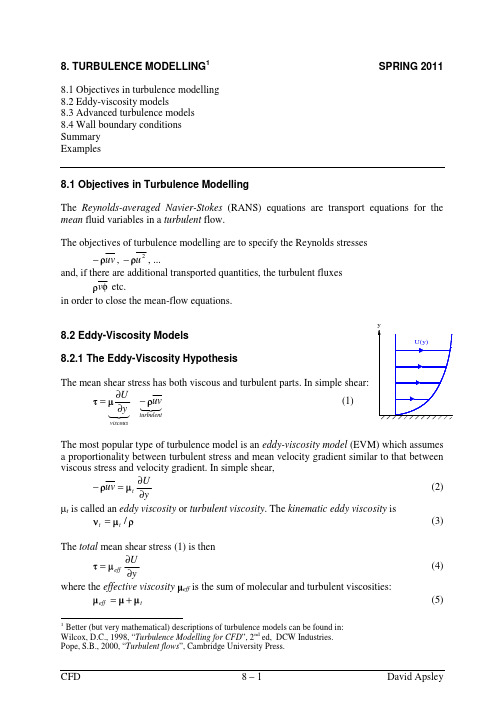
Aabort 异常中断, 中途失败, 夭折, 流产, 发育不全，中止计划[任务] accidentally 偶然地, 意外地accretion 增长activation energy 活化能active center 活性中心addition 增加adjacent 相邻的aerosol浮质(气体中的悬浮微粒,如烟,雾等), [化]气溶胶, 气雾剂, 烟雾剂Air flow circuits 气流循环ambient 周围的, 周围环境amines 胺amplitude 广阔, 丰富, 振幅, 物理学名词annular 环流的algebraic stress model(ASM) 代数应力模型algorithm 算法align 排列，使结盟, 使成一行alternately 轮流地analogy 模拟，效仿analytical solution 解析解anisotropic 各向异性的anthracite 无烟煤apparent 显然的, 外观上的，近似的approximation 近似arsenic 砷酸盐assembly 装配associate 联合，联系assume 假设assumption 假设atomization 雾化axial 轴向的Axisymmetry 轴对称的BBaffle 挡流板battlement 城垛式biography 经历bituminous coal 烟煤blow-off water 排污水blowing devices 鼓风(吹风)装置body force 体积力boiler plant 锅炉装置（车间）Boiling 沸腾Boltzmann 玻耳兹曼Bounded central differencing：有界中心差分格式Brownian rotation 布朗转动bulk 庞大的bulk density 堆积密度burner assembly 燃烧器组件burnout 燃尽Ccapability 性能，（实际）能力，容量，接受力carbon monoxide COcarbonate 碳酸盐carry-over loss 飞灰损失Cartesian 迪卡尔坐标的casing 箱，壳，套catalisis 催化channeled 有沟的，有缝的char 焦炭、炭circulation circuit 循环回路circumferential velocity 圆周速度clinkering 熔渣clipped 截尾的clipped Gaussian distribution 截尾高斯分布closure (模型的)封闭cloud of particles 颗粒云close proximity 距离很近cluster 颗粒团coal off-gas 煤的挥发气体coarse 粗糙的coarse grid 疏网格，粗网格Coatingcoaxial 同轴的coefficient of restitution 回弹系数；恢复系数coke 碳collision 碰撞competence 能力competing process 同时发生影响的competing-reactions submodel 平行反应子模型component 部分分量composition 成分computational expense 计算成本cone shape 圆锥体形状configuration 布置，构造confined flames 有界燃烧confirmation 证实, 确认, 批准Configuration 构造，外形conservation 守恒不灭conservation equation 守恒方程conserved scalars 守恒标量considerably 相当地consume 消耗contact angle 接触角contamination 污染contingency 偶然, 可能性, 意外事故, 可能发生的附带事件continuum 连续体Convection 对流converged 收敛的conveyer 输运机convolve 卷cooling duct 冷却管cooling wall 水冷壁coordinate transformation 坐标转换correlation 关联(式)correlation function 相关函数corrosion 腐蚀，锈coupling 联结, 接合, 耦合Cp：等压比热crack 裂缝，裂纹creep up （水）渗上来，蠕升critical 临界critically 精密地cross-correlation 互关联cumulative 累积的curtain wall 护墙，幕墙curve 曲线custom 习惯, 风俗, <动词单用>海关, (封建制度下)定期服劳役, 缴纳租税, 自定义, <偶用作>关税v.定制, 承接定做活的Cyan青色cyano 氰（基），深蓝，青色cyclone 旋风子，旋风，旋风筒cyclone separator 旋风分离器[除尘器]cylindrical 柱坐标的cylindrical coordinate 柱坐标Ddead zones 死区decompose 分解decouple 解藕的defy 使成为不可能Deforming：变形demography 统计Density：密度deposition 沉积derivative with respect to 对…的导数derivation 引出, 来历, 出处, (语言)语源, 词源design cycle 设计流程desposit 积灰，结垢deterministic approach 确定轨道模型deterministic 宿命的deviation 偏差devoid 缺乏devolatilization 析出挥发分，液化作用diffusion 扩散diffusivity 扩散系数digonal 二角(的), 对角的，二维的dilute 稀的diminish 减少direct numerical simulation 直接数值模拟discharge 释放discrete 离散的discrete phase 分散相, 不连续相discretization [数]离散化deselect 取消选定dispersion 弥散dissector 扩流锥dissociate thermally 热分解dissociation 分裂dissipation 消散, 分散, 挥霍, 浪费, 消遣, 放荡, 狂饮distribution of air 布风divide 除以dot line 虚线drag coefficient 牵引系数，阻力系数drag and drop 拖放drag force 曳力drift velocity 漂移速度driving force 驱[传, 主]动力droplet 液滴drum 锅筒dry-bottom-furnace 固态排渣炉dry-bottom 冷灰斗，固态排渣duct 管dump 渣坑dust-air mixture 一次风EEBU---Eddy break up 漩涡破碎模型eddy 涡旋effluent 废气，流出物elastic 弹性的electro-staic precipitators 静电除尘器emanate 散发, 发出, 发源，[罕]发散, 放射embrasure 喷口，枪眼emissivity [物]发射率empirical 经验的endothermic reaction 吸热反应enhance 增，涨enlarge 扩大ensemble 组，群，全体enthalpy 焓entity 实体entrain 携带，夹带entrained-bed 携带床Equation 方程equilibrate 保持平衡equilibrium 化学平衡ESCIMO-----Engulfment（卷吞）Stretching（拉伸）Coherence（粘附）Interdiffusion-interaction（相互扩散和化学反应）Moving-observer（运动观察者）exhaust 用尽, 耗尽, 抽完, 使精疲力尽排气排气装置用不完的, 不会枯竭的exit 出口，排气管exothermic reaction 放热反应expenditure 支出，经费expertise 经验explicitly 明白地, 明确地extinction 熄灭的extract 抽出，提取evaluation 评价，估计，赋值evaporation 蒸发(作用)Eulerian approach 欧拉法Ffacilitate 推动，促进factor 把…分解fast chemistry 快速化学反应fate 天数, 命运, 运气，注定, 送命，最终结果feasible 可行的，可能的feed pump 给水泵feedstock 填料Filling 倒水fine grid 密网格，细网格finite difference approximation 有限差分法flamelet 小火焰单元flame stability 火焰稳定性flow pattern 流型fluctuating velocity 脉动速度fluctuation 脉动，波动flue 烟道（气）flue duck 烟道fluoride 氟化物fold 夹层块forced-and-induced draft fan 鼓引风机forestall 防止Formulation:公式，函数fouling 沾污fraction 碎片部分，百分比fragmentation 破碎fuel-lean flamefuel-rich regions 富燃料区，浓燃料区fuse 熔化，熔融Ggas duct 烟道gas-tight 烟气密封gasification 气化(作用)gasifier 气化器Gauge 厚度，直径，测量仪表，估测。

JJMIE Volume 4, Number 3, June, 2010ISSN 1995-6665Pages 412 - 417 Jordan Journal of Mechanical and Industrial EngineeringSimulation and Modeling of Bubble Motion in an ElectrolyticBath of Soderberg PotC. Karuppannan, T.KannadasanCIT Sandwich Polytechnic College, Coimbatore-641 014, Tamilnadu, IndiaAbstract:In Aluminium manufacturing the Soderberg pot is widely used. The study explains about the bubble motion in cryolite liquid in a Soderberg pot anode face using comprehensive VOF multiphase model in FLUENT, under the action of gravitation. The distribution of bubbles introduced under the anodes of an aluminum reduction cell at the initial time has fixed size. 2D simulation results are reported for four cases with different initial conditions for the bubbles, physics and geometries.© 2010 Jordan Journal of Mechanical and Industrial Engineering. All rights reserved Keywords: Bubble analysis; Aluminium manufacturing;numerical simulation;VOF model.1.IntroductionIn aluminium manufacturing, formation of bubbles is amajor problem. Soderberg pots are used for themanufacture of aluminium. In Soderberg pot, the bubblesare formed in the interpolar distance and deposited on theanode face due to the thermal and chemical reactions in theelectrolytic bath. It reduces the input power and increasesthe energy consumption and reduces the current efficiency.Reduction in the formation of bubbles will increase thecurrent efficiency of the pot and output of aluminium.From the previous studies, the temperature distributionisclearly studied and proved. It has been reported thatformation of bubbles is from the anode surface. Hence, amodel of the anode surface is taken for the analysis. Initialdistributions of bubbles and diameters of the bubbles aretaken at random. Bubbles considered are having a non-zero density and deformable body; therefore having anappropriate mass (depending on the volume), henceproviding a more accurate mathematical model. With theaid of comprehensive Volume Of Fluid(VOF) model inFLUENT under the action of gravitation, the formedbubbles are coalescence and collapsed. The result iscompared with the mathematical model. The above workproves that the bubbles are collapsed with the increase inpressure in the feeding of Alumina. In this we can achievethe result accurately and enhance the current efficiencyand quality of Aluminium production.erning EquationsTo solve the given cryolite and bubble phase flow, fieldemploys the conservation equations for mass andmomentum for incompressible fluid.(1)(2)Momentum equations are solved for both cryolite andfluid. Continuum surface model (CSF) is used to describethe interfacial surface tension.(3)Equation (3) represents the VOF model governingequation for the cryolite-bubble phase model, wheredensity and viscosity are definedandPrimary volume fraction will be computed based on(4)3.Numerical SolutionProperties of cryolite and bubble used for the analysisare shown in Table 1. Model and meshing are done inGAMBIT.Table 1 Properties of Cryolite and BubbleProperty Cryolite Air (Bubble)Density2567 kg/m3 1.225 kg/m3Viscosity 1.57 cP0.017894 cPSurface Tension0.05 N/m(5)For interpolation of cryolite-bubble interface cellregion, Geometric Reconstruction Scheme is used. Thegeometric reconstruction scheme represents the interfacebetween fluids using a piecewise-linear approach. Whenthe cell is near the interface between two phases, thegeometric reconstruction scheme is used to obtain the facefluxes. It assumes that the interface between two fluids hasa linear slope within each cell, and uses this linear shape© 2010 Jordan Journal of Mechanical and Industrial Engineering. All rights reserved – Volume4, Number 3 (ISSN 1995-6665) 413for calculation of the advection of fluid through the cell faces. The first step in this reconstruction scheme is calculating the position of the linear interface relative to the center of each partially-filled cell, based on information about the volume fraction and its derivatives in the cell. The second step is calculating the amount of fluid through each face normally using the computed linear interface representation and information about the normal and tangential velocity distribution on the face. The third step is calculating the volume fraction in each cell using the balance of fluxes calculated during the previous step.Body force weighted scheme for differencing, Explicit scheme for temporal and PISO for pressure velocity coupling is used for solving. 4.Results & Discussions4.1.Case 1: Coalescence with Gravity: Small Bubble and Big Bubble BelowDomain dimensions are 20 mm x 10 mm surface. Geometry with three fluid zones is modelled viz., Cryolite, Bigger bubble and smaller bubble. Bubble walls are marked as interior. Results at time steps 0s, 0.03s, 0.033s, 0.036s are shown.a) initial configuration at t = 0s b) t = 0.03st = 0.033s t = 0.036sFigure 4-1. Coalescence of two rigid circular bubbles. The contours of the bubbles as well as the fluid velocity vectors are shown.The above results show that the bubbles move throughthe cryolite medium towards upwards under the action of buoyancy since the system is in the gravitational field. The bubbles having a lower density than the surrounding liquid medium displace the liquid, volume equivalent to their own volume and this displaced liquid wants to push the bubble upwards so as to occupy its volume. This is in accordance with the Archimedes' principle. Also, bigger bubble moves faster than the smaller bubble due to different buoyant force exerted depending on their volume. This phenomenon therefore contributes to the different velocities of the bubbles.The coalescence occurs already at time 0.03 seconds as opposed to the results depicted in the paper (3). This can be just due to different densities of the continuous fluid (in our case cryolite) which causes different speeds being attained by the bubble, hence decreasing the time to coalesce. The animation also shows the bigger bubble attaining a protruded shape in the beginning owing to being in the wake of the smaller bubble due to which it is in a low pressure region and gets specially pulled into the smaller bubble before coalescence occurs. These findingscan be verified by the paper (3).Figure 4-2. Typical C-shape morphology attained by the smaller bubble. Protruding shape of the bigger bubble,caught in the wake of the rising smaller bubble4.2.Case 2: Surface Tension Effect: Single EllipticalBubble with Different Surface Tension Values of the FluidDomain dimensions are 20 mm x 12 mm. Normalbubble rising problem with constant surface tensionspecification (0.05 N/m). Results at time steps t = 0.1s, t =0.1s, t = 0.05s are shown.© 2010 Jordan Journal of Mechanical and Industrial Engineering. All rights reserved – Volume4, Number 3 (ISSN 1995-6665)414a) initial configuration, t=0sb) bubble configuration at t = 0.1s, αs= 0.05 N/mc) t = 0.1s, αs= 0.005 N/md) time 0.05s, αs = 0.0005 N/mFigure 4-3. Influence of the surface tension coefficient αsThe above results match with the results of the publication qualitatively, although the more intricate details like bubble break-up owing to lower surface tension (figure 2.1(c)) have not been captured in the paper. Besides, the C-shape morphology attained due to the low pressure region in the wake of the rising bubble has been captured much better in the FLUENT simulation. The velocity vector plots overlaid on the bubble images for the four situations explain these phenomena .Bubble configurations at a) t = 0.1s, αs= 0.05 N/mb) t = 0.1s, αs= 0.005 N/m;c) time 0.05s, αs = 0.0005 N/mFigure 4-4. Rising bubbles attaining different shapes owing to the recirculation zone below themThese results are in perfect harmony with the simulation results of the independent group which was mentioned earlier (3).4.3. Case 3: Rigid Ellipsoidal Bubble Rising Around an Angular WallDomain dimensions are 2 x 2 cm with two angled walls Normal bubble rising problem with constant surface tension specification (0.05 N/m). Surface tension was included to come closer to the case description. Due tosurface tension, the bubble tends to attain minimum surface area as the liquid has a phobia towards it. As the surface tension value is quite high in our case, the bubble should not undergo easy break-up.© 2010 Jordan Journal of Mechanical and Industrial Engineering. All rights reserved – Volume4, Number 3 (ISSN 1995-6665)415(a) t = 0 s(b) t = 0.09 s(c) t = 0.18 s(d) t = 0.27 s(e) t = 0.36 s (f) t = 0.45 sFigure 4-5. Air bubble position at different times under stronger surface tension effects The bubble is at different positions compared to theliterature values. This must be due to different densitiesbeing taken for the liquid phase (our liquid is cryolite). Asthe surface tension effects are considerable, the bubbletends to avoid contact with the liquid (and rather preferscontact with the wall) while moving up under the action ofbuoyancy. The following images show the bubblebehaviour for weaker surface tension effects of the liquid,where the bubble does not necessarily oppose contact withthe liquid while moving up due to buoyancyFigure 4-6. Air bubble position at different times under weaker surface tension effects4.4. Case 4: Around 20 Bubbles with Random Distribution Rising in a ColumnDomain dimensions are 8 cm x 4 cm. 20 numbers of bubbles are taken for the analysis. Analysis is done for 27 time steps(a) t = 0 s(b) t = 0.15 s(c) t = 0.6 s(d) t = 0.9 sFigure 4-7 .Twenty air bubbles coalescing and rising under strong surface tension and buoyancy effectThe results show that the buoyant force acts on all of the bubbles and pushes them upwards. It is also visible thatthe bubbles below are caught up in the wake of the onesabove them and are pulled towards such low pressure areasdue to which they end up moving even in a zigzag fashion. The surface tension value being high, results in the bubblescoalescing as the liquid would prefer to minimize the surface contact area with the bubbles. As a result, the number of bubbles reduces drastically and ultimately there is an air column formed in the top region of the column. Some of the small bubbles are caught up in the eddies and tend to remain for relatively longer period within the liquid as they easily give-in to the fluid behavior due to their own lower inertia 5. Conclusion: Since the results obtained by the VOF multiphase model of FLUENT demonstrate the typical C-shape morphology of the bubbles as they rise up the column (as evident from the animation), the FLUENT results are much more accurate compared to the simplified mathematical model applied in the publication. Multi bubble analysis shows the real effect of bubble in the bottom of the anode plate in soderberg pot. The formed bubbles are collapsed with the aid of increasing the pressure in the feeding of Alumina and prevent the bubbles deposited on the anode surface. Hence, we can obtain the minimum energy consumption and enhance the current efficiency in the soderberg pot. References[1] A New Study On Bubble Behavior On Carbon Anode InAluminum Electrolysis. Gao, Bingliang, et al. [ed.] Halvor Kvande. s.l. : TMS (The Minerals, Metals & Materials Society), Light Metals 2005. [2] Numerical Simulation Of Bubble Coalescence Using AVolume Of Fluid (Vof) Model. Delnoij, E, Kuipers, J.A.M. and Van Swaaij, W. P. Lyon : s.n., 1998. Third International Conference on Multiphase Flow, ICMF’98. [3] A New Modelling For Simulating Bubble Motions In ASmelter. Michel, V. Romerio, Alexei, Lozinski and Jacques, Rappaz. [ed.] Halvor Kvande. s.l. : The Minerals, Metals &Materials Society), Light Metals 2005.(a) t = 0.09 s(b) t = 0.12 s(c) t = 0.18 s(d) t = 0.21 s© 2010 Jordan Journal of Mechanical and Industrial Engineering. All rights reserved – Volume4, Number 3 (ISSN 1995-6665) 416[4] B. Glorieux et al., “Density of Superheated and UndercooledLiquid Alumina by a Cont actless Method”, Int. J.Thermophys., Vol. 20, No. 4, 1999, 1085 – 1094. [5]T.J.Chung, Computational Fluid Dynamics, Cambridge, UK,Cambridge University Press, 2002.[6]M.Dupuis, “Computation of Aluminum reduction CellEnergy Balance Using ANSYS® Finite Elem ent Models”, TMS Light Metals, 1998, 409 – 417.[7]M. Dupuis and al., “Cathode Shell Stress Modelling”, TMSLight Metals, 1991, 427 – 430.[8]M. Dupuis, “ Computation of Accurate Horizonta l CurrentDensity on Metal Pad Using a Full Quarter Cell Thermo-electric Model”, CIM Light Metals, 2001, 3-11.[9]M. Dupuis and I. Tabsh, “Thermo-Electro-MagneticModeling of a Hall-Heroult Cell”, Proceeding of the ANSYS ® Magnetic Symposium, 1994, 9.3 – 9.13.[10]M. Segatz and D.Vogelsang, “Effect of Steel Parts onMagnetic Fields in Aluminum Reduc tion Cells”, TMS Light Metals, 1991, 393 – 398.[11]D.Richard and al., “Thermo-electro-mechanical Modelling ofthe Contact between Steel and Carbon Cylinders using the Finite Elem ent Method”, TMS Light Metals, 2000, 523-528. [12] I.Eick and D.V ogelsang, “Dimensioning of Cooling Fins forHigh –Amperage Reduc tion Cells”, TMS Light Metals, 1999, 339 – 345.[13]C.Vanvoren and al., “AP 50: The Pechiney 500 kA cell”,TMS Light Metals, 2001, 221 -226.[14]H.Kvande and W.Haupin, “Inert Anodes for AI Smelters:Energy Balance and Environmental Impact” JOM, Vol. 53, No. 5, 2001, 29-33.[15]Bruggeman and D.J.Danka, “Two-Dimensional ThermalModelling of the Hall-Heroult Cell”, Light Metals, 1990, 203-209.[16]Schmidt-Hatting and al., “Heat Losses of Different Pots”.Light Metals, 1985, 609-624.[17]Antille and al., “Effects of Current Increase of AluminiumReduction Cells”, Light Metals, 1995, 315-321.。

Shock Waves(2008)17:409–419DOI10.1007/s00193-008-0124-3ORIGINAL ARTICLENumerical investigation of ethyleneflame bubble instability induced by shock wavesGang Dong·Baochun Fan·Jingfang YeReceived:3August2006/Revised:28November2007/Accepted:26February2008/Published online:19March2008©Springer-Verlag2008Abstract In this paper,the ethylene/oxygen/nitrogen premixedflame instabilities induced by incident and reflec-ted shock wave were investigated numerically.The effects of grid resolutions and chemical mechanisms on theflame bubble deformation process are evaluated.In the computatio-nal frame,the2D multi-component Navier–Stokes equations with second-orderflux-difference splitting scheme were used;the stiff chemical source term was integrated using an implicit ordinary differential equations(ODEs)solver.The two ethylene/oxygen/nitrogen chemical mechanisms,namely 3-step reduced mechanism and35-step elementary skeletal mechanism,were used to examine the reliability of chemis-try.On the other hand,the different grid sizes, x× y= 0.25×0.5mm and x× y=0.15×0.2mm,were imple-mented to examine the accuracy of the grid resolution.The computational results were qualitatively validated with expe-rimental results of Thomas et al.(Combust Theory Model 5:573–594,2001).Two chemical mechanisms and two grid resolutions used in present study can qualitatively reproduce the ethylene sphericalflame instability process generated by an incident shock wave of Mach number1.7.For the case of interaction between theflame and reflected shock waves, the35-steps mechanism qualitatively predicts the physical process and is somewhat independent on the grid resolutions, while the3-steps mechanism fails to reproduce the instability Communicated by J.F.L.Haas.G.Dong(B)·B.Fan·J.YeState Key Laboratory of Transient Physics,Nanjing University of Science and Technology,Nanjing,Jiangsu210094,People’s Republic of Chinae-mail:dgvehicle@G.DongState Key Laboratory of Explosion Science and Technology,Beijing Institute of Technology,Beijing100081,China of ethyleneflame for the two selected grid resolutions.It is concluded that the detailed chemical mechanism,which includes the chain elementary reactions of fuel combustion, describes theflame instability induced by shock wave,in spite of the fact that theflame thickness(reaction zone)is represented by1–2grids only.Keywords Ethyleneflame·Shock waves·Chemical mechanism·Grid resolutionPACS82.40.Fp·47.40.Nm·47.70.Pq1IntroductionThe interactions between shock wave and curving contact discontinuity(e.g.,cylindrical or spherical gas with different density)can lead to the Richtmyer–Meshkov instability and further enhance the mixing process of gases with the different densities.The phenomenon occurs frequently in many prac-tice processes such as Scramjet[1,2].For example,theflame instability induced by shock wave can lead to the enhance-ment of the fuel/oxidizer mixing and the increase offlame burning rate.Many studies have been focused on the issues. For the inert shock–bubble interaction case,many experi-mental(e.g.,[3,4])and numerical(e.g.,[5–8])studies have been presented within a wide range of shock wave Mach number.In these studies,the fundamental mechanisms asso-ciated with the interface instability,the vortices structure and the mixing were widely investigated.The shock–bubble interaction has been proposed as a benchmark problem for testing the numerical scheme and grid resolution in CFD [9].On the other hand,for the reactive shock–flame inter-action case,Markstein’s classical experiments[10]showed the interactions offlames with a weak shock wave and its410G.Dong et al. reflected wave for butane/air mixture.Theflame instabi-lities were clearly observed.Recently,Thomas et al.[11]performed a series of experiments which showed the signi-ficantflame acceleration induced by stronger shock wavein C2H4/O2/N2mixture.They also showed that detonationcan emerge near the reaction zone for higher incident shockwave intensity.Numerical investigations on the interactionof shock wave withflame bubble have also been reportedwidely.Picone et al.[12],firstly,reported the interaction ofhot bubble with shock wave.However,the contact disconti-nuity in their model is inert.Ton et al.[13]studied the effectof chemical reaction during the interaction between the shockwave andflame.Khokhlov et al.[14]numerically studied asingle interaction of an incident shock wave with a sinusoi-dally perturbedflame.They developed a2D reactive Navier–Stokes equations solver based on the second-order Godunovtype scheme and the adaptive mesh refinement(AMR)tech-nique.Their results revealed that theflame instability and theenhancement of burned/unburned material mixing are due tothe Richtmyer–Meshkov(RM)instability.In their followingpapers[15–17],reflected shock wave effects were furtherconsidered using the same solver.The multiple shock–flameinteractions,through RM instability,result in the highly dis-tortedflame and further lead to the deflagration-to-detonation(DDT)at the specified conditions.Khokhlov et al.’s numeri-cal investigations represent a state of the art computation ontheflame instability perturbed by shock wave.However,as aone-step lumped reaction mechanism based on the Arrheniusform was used in their model,the effect of elementary reac-tion mechanisms for hydrocarbon fuel on the shock–flameinteraction has not been taken into account.In the present paper,a shock–flame interaction processis presented numerically considering the elementary chemi-cal reactions for ethylene fuel.The effects of the differentchemical reaction mechanisms and the grid resolutions onthe shock–flame interaction are evaluated in the numericalsimulations.The experiment of the ethyleneflame bubbleinstability perturbed by shock wave by Thomas et al.[11]has been used to validate and examine the numerical results.2Numerical methods2.1Governing equationsIn the numerical model,it is assumed that the thermally per-fect ideal gas law is used,thus,the2D axisymmetric reactiveNavier–Stokes equations for multi-component system are asfollows∂U ∂t +∂(F−F D)∂x+∂(G−G D)∂y+W=S(1)where,U denotes the solutions of the Eq.(1);F and G denote the convectionfluxes in x and y directions,respectively;F D and G D denote the transportfluxes in x and y directions, respectively;W denotes the axisymmetric correction term;S denotes the chemical source term.These terms can be expres-sed asU=⎛⎜⎜⎜⎜⎜⎜⎜⎝ρ1...ρKρuρvE⎞⎟⎟⎟⎟⎟⎟⎟⎠,F=⎛⎜⎜⎜⎜⎜⎜⎜⎝ρ1u...ρK uρuu+pρv u+pu(p+E)⎞⎟⎟⎟⎟⎟⎟⎟⎠,G=⎛⎜⎜⎜⎜⎜⎜⎜⎝ρ1v...ρK vρu v+pρvv+pv(p+E)⎞⎟⎟⎟⎟⎟⎟⎟⎠,W=vy⎛⎜⎜⎜⎜⎜⎜⎜⎝ρ1...ρKρuρvp+E⎞⎟⎟⎟⎟⎟⎟⎟⎠,F D=⎛⎜⎜⎜⎜⎜⎜⎜⎝ρD1∂(Y1)/∂x...ρD K∂(Y K)/∂xτxxτxyQ x+uτxx+vτxy⎞⎟⎟⎟⎟⎟⎟⎟⎠,G D=⎛⎜⎜⎜⎜⎜⎜⎜⎝ρD1∂(Y1)/∂y...ρD K∂(Y K)/∂yτyxτyyQ y+uτyx+vτyy⎞⎟⎟⎟⎟⎟⎟⎟⎠,S=⎛⎜⎜⎜⎜⎜⎜⎜⎝˙ω1...˙ωK⎞⎟⎟⎟⎟⎟⎟⎟⎠(2) whereρis the density of the mixture,ρ=Kk=1ρk,ρk=ρY k,Y k is the mass fraction for the species k;u and v are theflow velocities in x and y directions,respectively;p is the pressure;E is the total energy per unit volume,E=ρKk=1Y k e k+ρu2+v2/2;e k is the internal energy of the species k.All of thermodynamic properties in Eqs.(2) are deduced from the thermochemical polynomial descri-bed by Gordon and McBride[18].For the transport proper-ties in Eqs.(2),τxx,τyy andτxy are the normal stress and shear stress involved the molecular viscosity coefficient,µ, of the mixture,respectively;Q x= ∂T∂x+ρKk=1h k D k∂Y k∂x, Q y= ∂T∂y+ρKk=1h k D k∂Y k∂y, is the thermal conductivity of the mixture,h k is the enthalpy of the species k,T is the temperature of the mixture;D k is the diffusion coefficients of the species k.All of the transport properties are obtained from the gas-phase transport library of Kee et al.[19].As a chemical kinetic parameter,˙ωk is the net chemical produc-tion rate for species k in the elemental reactions which are interpreted and processed by the CHEMKIN-II package[20].Numerical investigation of ethyleneflame bubble instability induced by shock waves4112.2Numerical approachesA time splitting technique is used to solve the Eq.(1).Thesolutions of U at the n+1-th time step can be expressed asfollowsU n+1=L F L G L F D L G D L S L W U n(3)where,the terms L F and L G denote the operators of convec-tion computations in x and y directions,respectively;theterms L FD and L GDdenote the operators of transport com-putations in x and y directions,respectively;the term L S and L W denote the operators of chemical computation and axisymmetric correction,respectively.To capture the shock and contact discontinuity accura-tely,a second-order wave propagation algorithm based on theflux-difference splitting scheme and the Roe’s approxi-mate Riemann solver for the hyperbolic system of conserva-tion law,proposed by Leveque[21],is improved to meet the convection process(L F and L G in Eq.3)for multi-component system.In addition,a Superbee limiter with the total variation diminishing(TVD)is included to prevent the occurrence of the oscillations of the solutions at thefluid interfaces produced by shock wave and low-densityflame bubble during the shock–flame interaction simulations pre-sented in the next section.Transport process(L FD and L GDin Eq.3)is approximatedin terms of the second-order centered difference scheme.Axi-symmetric correction(L W in Eq.3)is solved using second-order Runge–Kutta methods.The solutions due to chemical reaction source term(L S in Eq.3)at one time step, t,can be expressed as followsU n+1k=U n k+˙ωk t.(4) Due to the different chemical characteristic time scales for the species in the reactiveflow,chemical stiffness arises.Hence, the LSODE solver[22]based on the implicit Gear algorithm is used to integrate the Eq.(4).For the computations of Eqs.(2)at the one time step,atten-tion should be paid to the solution of temperature.During the convection and axisymmetric correction processes,the solution of temperature is obtained using Newton iteration technique,while during the chemical reaction process the solution of temperature is solved coupled with the solutions of species concentrations,that is,the stiff ODE equations involved in temperature and species concentrations are inte-grated.3Chemical kinetic mechanismsIn this study,the two different chemical kinetic mechanisms are used to examine the effect of chemistry on the ethylene flame bubble instability induced by incident and its reflected shock waves.For the ethyleneflame,the large detailed kine-tic mechanism(e.g.,[23–26])can dramatically increase the computational cost for the multi-dimensional reactingflow simulations.As a result,some simplified ethylene mecha-nisms are proposed.For example,Varatharajan and Williams [27]and Varatharajan et al.[28]developed a two-step reduced mechanism used to simulate ethylene ignition and detona-tion properties,according to the steady-state and partial-equilibrium approximations.Baurle et al.[29]developed a three-step mechanism and a ten-step mechanism for ethylene combustion for hypersonicflows in a scramjet combustor.In the present study,we used two different ethylene mecha-nisms.One is the three-step short mechanism proposed by Baurel et al.[29].This mechanism includes three elemen-tary reactions with6species,the reactants,C2H4and O2, are transformed into the major products,CO2and H2O,and minor products,CO and H2,through three selected elemen-tary reaction steps.Another is the skeletal mechanism,which proposed by Li et al.[30]and has successfully applied in prediction of ethylene detonation wave structure[31].This mechanism includes36irreversible elementary reactions and describes the chain reaction process such as C2H4consump-tion,O–H radical interactions,peroxides formations and con-sumptions,and other intermediates consumptions.Here we use a reversible reaction,H+C2H4(+M)=C2H5(+M),to replace the two irreversible reactions(R23and R30)of the original Li’s mechanism[30].Thus,the used mechanism, named35-step mechanism,includes34irreversible and1 reversible elementary reactions.Both mechanisms and their parameters are shown in Tables1and2,respectively.The validation of the chemical mechanisms used in present study wasfirstly performed by1D premixed laminarflame calculations.The calculated C2H4/air laminarflame speeds at the atmospheric pressure by the three-step mechanism and the35-step mechanism were compared with the expe-rimental data[33],as shown in Fig.1.It is shown that the premixedflame speeds by the35-step mechanism at the dif-ferent equivalence ratios show a reasonable agreement with the experimental data.While the three-step mechanism very much underpredicts the premixedflame speeds.Further,in order to determine the grid size for describing theflame thickness(reaction zone)in the2D computations for inter-action offlame bubble with shock waves,we also calcula-ted the1D laminar premixed ethyleneflame structure at the Table1Three-step short kinetic mechanism[29]Chemical reactions A(cm3mol−1s−1)b E a(kJ mol−1) R1C2H4+O2=2CO+2H22.10×10140.0149.729R22CO+O2=2CO23.48×10112.084.233R32H2+O2=2H2O3.00×1020−1.00.000412G.Dong et al.Table2Thirty-five-step skeletal kinetic mechanism[30] a,c,d The third body coefficient:CO=1.9,CO2=3.8,H2=2.5,H2O=12.0b The third body coefficient: CO=1.9,CO2=3.8,H2=2.5,H2O=16.3e The third body coefficient: CO=2.5,CO2=2.5,H2=1.9,H2O=12.0f Lindemann fall-off reaction: A0=6.37×1027,b0=−2.8,Ea0=−0.2;the third body coefficient:H2=2.0,CO=2.0,CO2=3.0,H2O=5.0.Data taken from Miller and Bowman[32]Chemical reactions A(cm3mol−1s−1)b E a(kJ mol−1) R1H+O2→OH+O3.52×1016−0.771.4R2OH+O→H+O21.15×1014−0.3−0.7R3OH+H2→H2O+H1.17×1091.315.2R4H2O+H→OH+H26.72×1091.384.5R5O+H2O→2OH7.60×1003.853.4R62OH→O+H2O2.45×10−14.0−19.0R7a H+O2+M→HO2+M6.76×1019−1.40.0R8HO2+H→2OH1.70×10140.03.7R9HO2+H→H2+O24.28×10130.05.9R10HO2+OH→H2O+O22.89×10130.0−2.1R112HO2→H2O2+O23.02×10120.05.8R12b H2O2+M→2OH+M1.20×10170.0190.0R13c H+OH+M→H2O+M2.20×1022−2.00.0R14d H2O+M→H+OH+M2.18×1023−1.9498.4R15CO+OH→CO2+H4.40×1061.5−3.1R16CO2+H→CO+OH4.97×1081.589.6R17C2H4+O2→C2H3+HO24.22×10130.0241.0R18C2H4+OH→C2H3+H2O2.70×1052.312.4R19C2H4+O→CH3+HCO2.25×1062.10.0R20C2H4+O→CH2HCO+H1.21×1062.10.0R21C2H4+HO2→C2H3+H2O22.23×10120.071.9R22C2H4+H→C2H3+H22.25×1072.155.9R23C2H3+H→C2H2+H23.00×10130.00.0R24C2H3+O2→CH2O+HCO1.70×1029−5.327.2R25C2H3+O2→CH2HCO+O7.00×1014−0.622.0R26CH3+O2→CH2O+OH3.30×10110.037.4R27CH3+O→CH2O+H8.43×10130.00.0R28C2H5+O2→C2H4+HO22.00×10120.020.9R29CH2HCO→CH2CO+H1.05×1037−7.2186.0R30CH2CO+H→CH3+CO1.11×1072.08.4R31CH2O+OH→HCO+H2O3.90×10100.91.7R32e HCO+M→CO+H+M1.86×1017−1.071.0R33HCO+O2→CO+HO23.00×10120.00.0R34C2H2+OH→CH2CO+H1.90×1071.74.2R35f H+C2H4(+M)=C2H5(+M)2.21×10130.08.6specified mixture(C2H4+3O2+4N2),initial temperature (550K)and pressure(13,160Pa)which are same as those in the shock–flame interaction experiment[11].As a baseline,a detailed chemical mechanism,the GRI mechanism30.0[26],was implemented to examine the three-step and35-step mechanisms in theflame structure calculations.As seen from Fig.2,the35-step mechanism shows the good agreements with GRI mechanism.The laminarflame thickness,determi-ned by the distance between the Y=0.95Y C2H4,0and Y=0.05Y C2H4,0(Y C2H4,0is the initial mass fraction of C2H4)intheflame[14],is0.787and0.783mm for the GRI mechanism and the35-step mechanism,respectively.Figure2a shows the vertical shadow bar which represents the ethyleneflame thi-ckness for the35-step mechanism.The three-step mechanism shows the widerflame thickness(4.232mm)and predicts the higher temperature and H2concentrations than those by the 35-step mechanism and GRI mechanism.In Fig.2d,the com-parison of heat release rate between the three-step mechanism and other two mechanisms also shows the difference.For the 35-step and GRI-Mech3.0mechanisms,a higher peak within the narrow region can be seen compared with the results of the three-step mechanism.the three-step and other two mechanisms in Fig.2are due to the simplicity of the three-step chemical kinetic mecha-nism.It is believed that the lack of chain branching reactions (R1in Table2)and the reactions of ethylene with highly length230mm in the test section of the shock tube.The initial flame center was located in the center of the window section, 135mm from the end wall.Figure3a gives the part of window section.In the present study,we use a computational domainFig.2One-dimensional laminarflame structure computed by the different chemical kinetic mechanisms for C2H4+3O2+4N2,T0=500K,p0=13,160Pa414G.Dong et al.Fig.3a initial experimental Schlieren image and b Computational domainwith height38mm and length180mm,which describes a2D axisymmetric region,as shown in Fig.3b.The length ofthe computational domain consists of135mm downstreamand45mm upstream offlame center.The half length of win-dow section is115mm,which is somewhat longer than thedownstream length offlame center as shown in Fig.3a.Thisis because thefinal10mm of window section was obscuredby aflangefitting in the experiment[11].The top and rightboundary is no-slip rigid adiabatic wall boundary condition.The left boundary is the inflow boundary conditions whichtheflow and thermodynamic properties before the arrival ofthe reflected shock wave arefixed to be theflow conditionbehind the incident shock wave.The bottom boundary is theaxis of symmetry.We choose thefirst Schlieren images sequence in theirseries of experiments(see[11,Fig.1])for validating thepresent simulations.In this experiment,an incident shockwave with Mach number1.7was produced by the high-pressure driver section of a shock tube.An electric discharge,which was used to ignite theflame bubble,was triggered bya pressure gauge coupled to a level-sensitive detector and adelay unit.When the pressure gauge detected the incidentshock wave,the delay was chosen so that aflame bubblewith desired diameter could be formed before the shockwave arrived at the ignition plane.Before the ignition,thetest section of the shock tube was evacuated and thenfilledto the C2H4+3O2+4N2mixture with the initial pressure of13,160Pa.Initially,the incident shock wave was locatedon the left of the ethyleneflame bubble(Fig.3)and sub-sequently moved to the right and through theflame bubble.When the shock wave reached the end wall and reboundedfrom it,a reflected shock wave formed and interacted withtheflame bubble again.The multiple shock–flame interac-tions can lead to the instability of theflame surface dueto Richtmyer–Meshkov effect.In the computations,the ini-tial time is same as the experimental time shown as Fig.3aand is set to0µs,the C2H4+3O2+4N2mixturefills the Table3Mixture compositionand thermodynamics parameterswithin the initialflame bubblea C p and C v are the specific heatcapacity at constant pressureand constant volume,respectively,for the mixturewithin the initialflame bubbleMixture mass fractionC2H40O20.113CO20.137H2O0.122CO0.150H20.004N20.474Density(kg m−3)0.0148Temperature(K)2,860a C p/C v 1.242Table4Computational runsRun Grid size Mechanism1 x× y=0.15×0.2mm35-step2 x× y=0.25×0.5mm35-step3 x× y=0.15×0.2mm3-step4 x× y=0.25×0.5mm3-stepwhole computational domain except for the initial bubble made of the combustion products.The temperature and pres-sure before the incident shock wave are T0=298K and p0=13,160Pa,respectively,as those in experiment[11]. The mixture composition and thermodynamic parameters within the initialflame bubble correspond to the adiaba-tic burning at constant pressure,as shown in Table3.The velocity of thefluid before the incident shock wave is zero. The mixture thermodynamic properties behind the shock wave can be calculated in terms of the Rankine–Hugoniot relationship with a given incident shock wave Mach num-ber.Four computational runs were performed to study the effects of chemical kinetic mechanism and grid size on the ethyleneflame instability,as shown in Table4.Beside two selected mechanisms(three-step and35-step mechanisms), two different grid resolutions, x× y=0.25×0.5mm and x× y=0.15×0.2mm,are used.For the coarse grid size andfine grid size,theflame thickness(reaction zone) can be represented by1–2grid width and3–4grid width, respectively,based on the premixedflame structure calcu-lations whichflame thickness is about0.787mm,as shown in Fig.2.The time-splitting scheme(also called Godunov-splitting scheme)comes from the computationalfluid dyna-mic(CFD)code by Leveque[35]and its temporal accuracy is proven to be sufficient[36].For all of the computatio-nal runs,the Courant–Friedrichs–Lewy(CFL)number is set to0.7.With the second-order spatial discretization and the reasonable temporal marching,the effect of numerical per-turbations on the bubble distortions produced by the initialNumerical investigation of ethylene flame bubble instability induced by shock waves415Fig.4Comparisons between the experimental Schlieren images [11]and computational Schlieren images for the interaction between the incident shock wave and flame bubble.The frame time is a 50µs,b 100µs,c 150µs and d 200µs.The Runs 1–4correspond to the com-putational images,as shown in Table 4.Incident shock Mach number is 1.7;mixture is C 2H 4+3O 2+4N 2flame interface cannot be obviously observed for all of com-putational runs with CFL =0.7.For the convenience of comparison,the numerical results are converted to the computational Schlieren images accor-ding to the formula [37]I =I 0 0.5+8max min cos θ∂ρ+sin θ∂ρ(5)where,I and I 0are the computational and initial light inten-sity,respectively;the θis the angle of the knife edge (fromthe horizontal);the ρmax and ρmin are the maximum and minimum density in the flow field.Figure 4gives the experi-mental and computational Schlieren images for case of inci-dent shock wave interaction with the flame bubble.In Fig.4,the experimental images are the 2D optical projection of 3D flame bubble,while the computational images are the 2D computational cutaway section of flame bubble.In addition,it should note that the Eq.5is less representative of actual Schlieren image in the present axisymmetric simulations than those in 2D cylinder.Although some differences between the experiments and computations exist due to the above men-tioned reasons,a qualitative similarity between the experi-mental observations and computational Schlieren images is observed.In the Fig.4a,the incident shock wave is halfway crossing the flame bubble,and the upstream interface of the flame bubble deforms.As time goes on,the flame bubble acquires a kidney shape,as shown in Fig.4b.At this time,the arc transmitted shock wave and foot structure due to the Mach reflection of the incident shock wave are also clearly shown in the both experimental and computational images.In the Fig.4c,a jet due to the Richtmyer–Meshkov instability occurs and breaks up the deformed flame bubble.Figure 4d416G.Dong et al.Fig.5Space–time diagrams of a35-step mechanism and b3-step mechanism for the shock–flame interaction.Incident shock Mach num-ber is1.7;mixture is C2H4+3O2+4N2.Grid resolution is x× y= 0.25×0.5mm.Lines are the computational results,symbols are theexperimental resultsshows the growth of the jet and the formation of the vortex structures due to the impingement of the jet on the downs-tream of theflame bubble at the later time.The comparisons between the experiments and compu-tations in Fig.4illustrate that all of the numerical simula-tions for selected chemical mechanisms and grid resolutions in the present study are capable of reproducing the experi-mental observations on the ethyleneflame bubble instability process perturbed by incident shock wave.Figure5gives the space–time diagram of tracing lines of shock front and left and right interfaces offlame for both mechanisms with x× y=0.25×0.5mm.One can see that even the coarseT/TAT/A56789101112130.050.10.1535-step,coarse g rids3-step,coarse g rids35-step,fine g rids3-step,fine g ridsFig.6Area ratio distributions of temperature forflame bubble instabi-lity induced by incident shock wave,the time corresponds to the Fig.4dgrid resolution is used,the interaction offlame with incident shock wave(below the290µs)shows the good agreement with the experimental results.It should be noted that the axi-symmetric boundary of the computational tube is only the approximation of the experimental shock tube with rectan-gular square cross section(76mm×38mm).However,the agreements between the experiments and computations in Fig.5imply that the axisymmetric assumption in the present study is acceptable.Further,in order to examine the effects of grid resolution and chemistry,we give the distributions of the2Dflame bubble area ratio of the different computational temperatures,as shown in Fig.6.In thisfigure,A T denotes the2Dflame bubble area of the temperature T,A denotes the total2Dflame bubble area which is defined by region of temperature between T/T0=5and13.The computational results show that the area ratio peak appears within tempera-ture range T/T0=10.5±0.5for all of four computational runs.The distributions imply that the major part offlame area concentrates in the narrow high-temperature range.The fur-ther observation shows that for both chemical mechanisms, computations using coarse grids give a more high tempera-ture area than those byfine grids.On the other hand,the three-step mechanism predicts the higher temperature than that by the35-step mechanism when grid resolution isfixed. In spite of the differences shown above,the all grid reso-lutions and chemical mechanisms in the present study can predict the similar interaction process between the incident shock wave andflame bubble.The similarity implies that the hydrodynamic process instead of the chemical process plays an important role in this case.The computations of interaction offlame bubble with the reflected shock wave show the distinguishing images forNumerical investigation of ethylene flame bubble instability induced by shock waves417Fig.7Comparisons between the experimental Schlieren images [11]and computational Schlieren images for the interaction between the reflected shock wave and flame bubble.The frame time is a 400µs,b 450µs and c 500µs.The Runs 1–4correspond to the computatio-nal images,as shown in Table 4.Incident shock Mach number is 1.7;mixture is C 2H 4+3O 2+4N 2different computational runs.Figure 7gives the sequential frames of reflected shock wave from end wall.In this case,the stagnant state of the fluid behind the reflected shock wave is formed so that the chemical reactions play an impor-tant role in the flame instability.As seen from experimental images of Fig.7,the deformed flame expands and develops towards left.The 35-step mechanism qualitatively predictsthe interaction process for both of grid resolutions (Runs 1and 2).Note that the minor discrepancies of flame shape between the experimental and computational images can be observed,since the computational flame shape based on the axisymmetric assumption is different from the actual one in which the expanded flame has partly touched to the optical window section of the shock tube after the reflected shock wave.Even through the minor discrepancies exist,the Run 1of fine grids shows the wrinkly flame interface and the qua-litative agreement with the experimental Schlieren image,Run 2of coarse grids also qualitatively describes the shape of deformed flame although it misses the subtle structure of flame interface.On the other hand,computational results by the three-step mechanism (Runs 3and 4)for both coarse and fine grids give the wrong images which seem that flame develops as the inert pocket without chemical activity.As can been seen from Fig.1and 2d,the three-step mechanism gives the lower flame speed and the lower heat release rate and thus slows the flame expansion process in the interaction process of Fig.7.In addition,Fig.5also shows the tracing lines of left and right interfaces of developing flame for both mecha-nisms after the shock wave reflects (beyond the 290µs).Note that there are no experimental data of right interface of flame owing to the optical obstruction by a flange fitting.However,it is believed that the right interface of the flame stays at the end wall of the test section after the shock wave reflection,as shown by the computational results.For 35-step mecha-nism as shown in Fig.5a,the computational tracing lines of reflected shock front and left interface of flame reasonably agree with the experiments.The computational distance bet-ween the left and right interfaces of flame increases when the time goes on,this also indicates that the flame expands after the reflected shock wave.For the three-step mechanism as shown in Fig.5b,flame expansion has not been occurred owing to the lower flame speed as illustrated by Fig.1.Also,the three-step mechanism underpredicts the reflected shock velocity and flame speed compared with the experiments.Figure 8shows the 2D flame area ratio distributions along with the flame temperature after the reflected shock wave.The results further illustrate that the different chemical mech-anisms show the remarkably difference in predicting the flame temperature.The 35-step mechanism for both coarse and fine grid resolutions gives the similar area ratio distribu-tion which the high temperature area (wide area ratio peak)concentrates in the temperature range of T /T 0=8−10.Generally,the computational results by 35-step mechanism are independent of the grid resolution.Whereas the three-step mechanism gives the different computational results for the different grid resolutions,which also implies that the three-step mechanism is sensitive to the grid resolutions.Figure 9gives the area ratio distributions of mass fractions of CO 2for both 35-step and three-step mechanism in the flame inter-acted by the reflected shock.For the 35-step mechanism,。

流体动力学fluid dynamics 连续介质力学mechanics of continuous media 介质medium 流体质点fluid particle无粘性流体nonviscous fluid, inviscid fluid 连续介质假设continuous medium hypothesis 流体运动学fluid kinematics 水静力学hydrostatics液体静力学hydrostatics 支配方程governing equation伯努利方程Bernoulli equation 伯努利定理Bernonlli theorem毕奥-萨伐尔定律Biot-Savart law 欧拉方程Euler equation亥姆霍兹定理Helmholtz theorem 开尔文定理Kelvin theorem涡片vortex sheet 库塔-茹可夫斯基条件Kutta-Zhoukowski condition 布拉休斯解Blasius solution 达朗贝尔佯廖d'Alembert paradox雷诺数Reynolds number 施特鲁哈尔数Strouhal number随体导数material derivative 不可压缩流体incompressible fluid质量守恒conservation of mass 动量守恒conservation of momentum能量守恒conservation of energy 动量方程momentum equation能量方程energy equation 控制体积control volume液体静压hydrostatic pressure 涡量拟能enstrophy压差differential pressure 流[动] flow流线stream line 流面stream surface流管stream tube 迹线path, path line流场flow field 流态flow regime流动参量flow parameter 流量flow rate, flow discharge涡旋vortex 涡量vorticity涡丝vortex filament 涡线vortex line涡面vortex surface 涡层vortex layer涡环vortex ring 涡对vortex pair涡管vortex tube 涡街vortex street卡门涡街Karman vortex street 马蹄涡horseshoe vortex对流涡胞convective cell 卷筒涡胞roll cell涡eddy 涡粘性eddy viscosity环流circulation 环量circulation速度环量velocity circulation 偶极子doublet, dipole驻点stagnation point 总压[力] total pressure总压头total head 静压头static head总焓total enthalpy 能量输运energy transport速度剖面velocity profile 库埃特流Couette flow单相流single phase flow 单组份流single-component flow均匀流uniform flow 非均匀流nonuniform flow二维流two-dimensional flow 三维流three-dimensional flow准定常流quasi-steady flow 非定常流unsteady flow, non-steady flow 暂态流transient flow 周期流periodic flow振荡流oscillatory flow 分层流stratified flow无旋流irrotational flow 有旋流rotational flow轴对称流axisymmetric flow 不可压缩性incompressibility不可压缩流[动] incompressible flow 浮体floating body定倾中心metacenter 阻力drag, resistance减阻drag reduction 表面力surface force表面张力surface tension 毛细[管]作用capillarity来流incoming flow 自由流free stream自由流线free stream line 外流external flow进口entrance, inlet 出口exit, outlet扰动disturbance, perturbation 分布distribution传播propagation 色散dispersion弥散dispersion 附加质量added mass ,associated mass收缩contraction 镜象法image method无量纲参数dimensionless parameter 几何相似geometric similarity运动相似kinematic similarity 动力相似[性] dynamic similarity平面流plane flow 势potential势流potential flow 速度势velocity potential复势complex potential 复速度complex velocity流函数stream function 源source汇sink 速度[水]头velocity head拐角流corner flow 空泡流cavity flow超空泡supercavity 超空泡流supercavity flow空气动力学aerodynamics低速空气动力学low-speed aerodynamics 高速空气动力学high-speed aerodynamics气动热力学aerothermodynamics 亚声速流[动] subsonic flow跨声速流[动] transonic flow 超声速流[动] supersonic flow锥形流conical flow 楔流wedge flow叶栅流cascade flow 非平衡流[动] non-equilibrium flow细长体slender body 细长度slenderness钝头体bluff body 钝体blunt body翼型airfoil 翼弦chord薄翼理论thin-airfoil theory 构型configuration后缘trailing edge 迎角angle of attack失速stall 脱体激波detached shock wave波阻wave drag 诱导阻力induced drag诱导速度induced velocity 临界雷诺数critical Reynolds number 前缘涡leading edge vortex 附着涡bound vortex约束涡confined vortex 气动中心aerodynamic center气动力aerodynamic force 气动噪声aerodynamic noise气动加热aerodynamic heating 离解dissociation地面效应ground effect 气体动力学gas dynamics稀疏波rarefaction wave 热状态方程thermal equation of state 喷管Nozzle 普朗特-迈耶流Prandtl-Meyer flow瑞利流Rayleigh flow 可压缩流[动] compressible flow可压缩流体compressible fluid 绝热流adiabatic flow非绝热流diabatic flow 未扰动流undisturbed flow等熵流isentropic flow 匀熵流homoentropic flow兰金-于戈尼奥条件Rankine-Hugoniot condition 状态方程equation of state量热状态方程caloric equation of state 完全气体perfect gas拉瓦尔喷管Laval nozzle 马赫角Mach angle马赫锥Mach cone 马赫线Mach line马赫数Mach number 马赫波Mach wave当地马赫数local Mach number 冲击波shock wave激波shock wave 正激波normal shock wave斜激波oblique shock wave 头波bow wave附体激波attached shock wave 激波阵面shock front激波层shock layer 压缩波compression wave反射reflection 折射refraction散射scattering 衍射diffraction绕射diffraction出口压力exit pressure 超压[强] over pressure反压back pressure 爆炸explosion爆轰detonation 缓燃deflagration水动力学hydrodynamics 液体动力学hydrodynamics泰勒不稳定性Taylor instability 盖斯特纳波Gerstner wave斯托克斯波Stokes wave 瑞利数Rayleigh number自由面free surface 波速wave speed, wave velocity波高wave height 波列wave train波群wave group 波能wave energy表面波surface wave 表面张力波capillary wave规则波regular wave 不规则波irregular wave浅水波shallow water wave深水波deep water wave 重力波gravity wave椭圆余弦波cnoidal wave 潮波tidal wave涌波surge wave 破碎波breaking wave船波ship wave 非线性波nonlinear wave孤立子soliton 水动[力]噪声hydrodynamic noise 水击water hammer 空化cavitation空化数cavitation number 空蚀cavitation damage超空化流supercavitating flow 水翼hydrofoil水力学hydraulics 洪水波flood wave涟漪ripple 消能energy dissipation海洋水动力学marine hydrodynamics 谢齐公式Chezy formula欧拉数Euler number 弗劳德数Froude number水力半径hydraulic radius 水力坡度hvdraulic slope高度水头elevating head 水头损失head loss水位water level 水跃hydraulic jump含水层aquifer 排水drainage排放量discharge 壅水曲线back water curve压[强水]头pressure head 过水断面flow cross-section明槽流open channel flow 孔流orifice flow无压流free surface flow 有压流pressure flow缓流subcritical flow 急流supercritical flow渐变流gradually varied flow 急变流rapidly varied flow临界流critical flow 异重流density current, gravity flow堰流weir flow 掺气流aerated flow含沙流sediment-laden stream 降水曲线dropdown curve沉积物sediment, deposit 沉[降堆]积sedimentation, deposition沉降速度settling velocity 流动稳定性flow stability不稳定性instability 奥尔-索末菲方程Orr-Sommerfeld equation 涡量方程vorticity equation 泊肃叶流Poiseuille flow奥辛流Oseen flow 剪切流shear flow粘性流[动] viscous flow 层流laminar flow分离流separated flow 二次流secondary flow近场流near field flow 远场流far field flow滞止流stagnation flow 尾流wake [flow]回流back flow 反流reverse flow射流jet 自由射流free jet管流pipe flow, tube flow 内流internal flow拟序结构coherent structure 猝发过程bursting process表观粘度apparent viscosity 运动粘性kinematic viscosity动力粘性dynamic viscosity 泊poise厘泊centipoise 厘沱centistoke剪切层shear layer 次层sublayer流动分离flow separation 层流分离laminar separation湍流分离turbulent separation 分离点separation point附着点attachment point 再附reattachment再层流化relaminarization 起动涡starting vortex驻涡standing vortex 涡旋破碎vortex breakdown涡旋脱落vortex shedding 压[力]降pressure drop压差阻力pressure drag 压力能pressure energy型阻profile drag 滑移速度slip velocity无滑移条件non-slip condition 壁剪应力skin friction, frictional drag 壁剪切速度friction velocity 磨擦损失friction loss磨擦因子friction factor 耗散dissipation滞后lag 相似性解similar solution局域相似local similarity 气体润滑gas lubrication液体动力润滑hydrodynamic lubrication 浆体slurry泰勒数Taylor number 纳维-斯托克斯方程Navier-Stokes equation 牛顿流体Newtonian fluid 边界层理论boundary later theory边界层方程boundary layer equation 边界层boundary layer附面层boundary layer 层流边界层laminar boundary layer湍流边界层turbulent boundary layer 温度边界层thermal boundary layer边界层转捩boundary layer transition 边界层分离boundary layer separation边界层厚度boundary layer thickness 位移厚度displacement thickness动量厚度momentum thickness 能量厚度energy thickness焓厚度enthalpy thickness 注入injection吸出suction 泰勒涡Taylor vortex速度亏损律velocity defect law 形状因子shape factor测速法anemometry 粘度测定法visco[si] metry流动显示flow visualization 油烟显示oil smoke visualization孔板流量计orifice meter 频率响应frequency response油膜显示oil film visualization 阴影法shadow method纹影法schlieren method 烟丝法smoke wire method丝线法tuft method 氢泡法nydrogen bubble method相似理论similarity theory 相似律similarity law部分相似partial similarity 定理pi theorem, Buckingham theorem 静[态]校准static calibration 动态校准dynamic calibration风洞wind tunnel 激波管shock tube激波管风洞shock tube wind tunnel 水洞water tunnel拖曳水池towing tank 旋臂水池rotating arm basin扩散段diffuser 测压孔pressure tap皮托管pitot tube 普雷斯顿管preston tube斯坦顿管Stanton tube 文丘里管Venturi tubeU形管U-tube 压强计manometer微压计micromanometer 多管压强计multiple manometer静压管static [pressure]tube 流速计anemometer风速管Pitot- static tube 激光多普勒测速计laser Doppler anemometer, laser Doppler velocimeter 热线流速计hot-wire anemometer热膜流速计hot- film anemometer 流量计flow meter粘度计visco[si] meter 涡量计vorticity meter传感器transducer, sensor 压强传感器pressure transducer热敏电阻thermistor 示踪物tracer时间线time line 脉线streak line尺度效应scale effect 壁效应wall effect堵塞blockage 堵寒效应blockage effect动态响应dynamic response 响应频率response frequency底压base pressure 菲克定律Fick law巴塞特力Basset force 埃克特数Eckert number格拉斯霍夫数Grashof number 努塞特数Nusselt number普朗特数prandtl number 雷诺比拟Reynolds analogy施密特数schmidt number 斯坦顿数Stanton number对流convection 自由对流natural convection, free convec-tion强迫对流forced convection 热对流heat convection质量传递mass transfer 传质系数mass transfer coefficient热量传递heat transfer 传热系数heat transfer coefficient对流传热convective heat transfer 辐射传热radiative heat transfer动量交换momentum transfer 能量传递energy transfer传导conduction 热传导conductive heat transfer热交换heat exchange 临界热通量critical heat flux浓度concentration 扩散diffusion扩散性diffusivity 扩散率diffusivity扩散速度diffusion velocity 分子扩散molecular diffusion沸腾boiling 蒸发evaporation气化gasification 凝结condensation成核nucleation 计算流体力学computational fluid mechanics 多重尺度问题multiple scale problem 伯格斯方程Burgers equation对流扩散方程convection diffusion equation KDU方程KDV equation修正微分方程modified differential equation 拉克斯等价定理Lax equivalence theorem 数值模拟numerical simulation 大涡模拟large eddy simulation数值粘性numerical viscosity 非线性不稳定性nonlinear instability希尔特稳定性分析Hirt stability analysis 相容条件consistency conditionCFL条件Courant- Friedrichs- Lewy condition ,CFL condition狄里克雷边界条件Dirichlet boundarycondition熵条件entropy condition 远场边界条件far field boundary condition流入边界条件inflow boundary condition无反射边界条件nonreflecting boundary condition数值边界条件numerical boundary condition流出边界条件outflow boundary condition冯.诺伊曼条件von Neumann condition 近似因子分解法approximate factorization method 人工压缩artificial compression 人工粘性artificial viscosity边界元法boundary element method 配置方法collocation method能量法energy method 有限体积法finite volume method流体网格法fluid in cell method, FLIC method通量校正传输法flux-corrected transport method通量矢量分解法flux vector splitting method 伽辽金法Galerkin method积分方法integral method 标记网格法marker and cell method, MAC method 特征线法method of characteristics 直线法method of lines矩量法moment method 多重网格法multi- grid method板块法panel method 质点网格法particle in cell method, PIC method 质点法particle method 预估校正法predictor-corrector method投影法projection method 准谱法pseudo-spectral method随机选取法random choice method 激波捕捉法shock-capturing method激波拟合法shock-fitting method 谱方法spectral method稀疏矩阵分解法split coefficient matrix method 不定常法time-dependent method时间分步法time splitting method 变分法variational method涡方法vortex method 隐格式implicit scheme显格式explicit scheme 交替方向隐格式alternating direction implicit scheme, ADI scheme 反扩散差分格式anti-diffusion difference scheme紧差分格式compact difference scheme 守恒差分格式conservation difference scheme 克兰克-尼科尔森格式Crank-Nicolson scheme杜福特-弗兰克尔格式Dufort-Frankel scheme指数格式exponential scheme 戈本诺夫格式Godunov scheme高分辨率格式high resolution scheme 拉克斯-温德罗夫格式Lax-Wendroff scheme 蛙跳格式leap-frog scheme 单调差分格式monotone difference scheme保单调差分格式monotonicity preserving diffe-rence scheme穆曼-科尔格式Murman-Cole scheme 半隐格式semi-implicit scheme斜迎风格式skew-upstream scheme全变差下降格式total variation decreasing scheme TVD scheme迎风格式upstream scheme , upwind scheme计算区域computational domain 物理区域physical domain影响域domain of influence 依赖域domain of dependence区域分解domain decomposition 维数分解dimensional split物理解physical solution 弱解weak solution黎曼解算子Riemann solver 守恒型conservation form弱守恒型weak conservation form 强守恒型strong conservation form散度型divergence form 贴体曲线坐标body- fitted curvilinear coordi-nates [自]适应网格[self-] adaptive mesh 适应网格生成adaptive grid generation自动网格生成automatic grid generation 数值网格生成numerical grid generation交错网格staggered mesh 网格雷诺数cell Reynolds number数植扩散numerical diffusion 数值耗散numerical dissipation数值色散numerical dispersion 数值通量numerical flux放大因子amplification factor 放大矩阵amplification matrix阻尼误差damping error 离散涡discrete vortex熵通量entropy flux 熵函数entropy function分步法fractional step method。