ACM 计算几何 最小圆覆盖算法

最少顶点覆盖问题的研究作者：张惠玲谢邱敏李炜来源：《中国新通信》2014年第13期【摘要】对此最少顶点覆盖问题，我们巧妙提出了两种方法：1）建立整数规划模型，用分支定界算法求解模型;2）将其转换成最小支配集问题，最小支配集问题是NP完全问题，找不到多项式时间算法，我们分别采用贪心算法和近似算法（经典的遗传算法）求解。

在此基础上，我们还分析了两种方法的优缺点并将模型推广使用。

【关键词】最少顶点覆盖整数规划最小支配集贪心算法近似算法一、问题简述考虑如下数学问题：现有一片的矩形网络图，给定67个顶点的位置坐标，现要选取其中的某些顶点作为圆心，以20为半径作圆，要求能覆盖全部顶点，求要选取顶点的最少数目，画出覆盖图形。

（如图1）【67个顶点的坐标分别为（10，115），（33，26），（58，141），（0，19），（1，170），（77，149），（80，68），（46，46），（91，111），（70，56），（91，127），（75，180），（71，163），（16，141），（34，123），（45，15），（44，92），（34，183），（33，75），（17，181），（15，26），（57，70），（92，82），（97，182），（29，97），（64，7），（1，94），（37，149），（19，199），（56，157），（85，192），（82，39），（75，134），（96，65），（97，42），（50，128），（68，112），（80，6），（40，197），（96，13），（86，96），（44，61），（45，170），（99，143），（20，6），（4，151），（1，135），（0，54），（65，35），（48，113），（77，83），（30，55），（76，23），（49，30），（58，85），（62，188），（12，43），（1，190），（35，0），（69，97），（9，67），（21，165），（90，165），（16，88），（4，3），（99，198），（27，40）】二、模型建立2.1 基于整数规划模型求解小规模最少顶点覆盖问题以所选顶点个数最少为目标函数，约束条件是使得每个顶点都被覆盖。

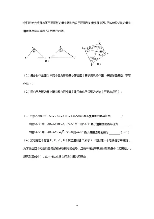
我们将能完全覆盖某平面图形的最小圆称为该平面图形的最小覆盖圆。

例如线段AB的最小覆盖圆就是以线段AB为直径的圆。

（1）请分别作出图1中两个三角形的最小覆盖圆（要求用尺规作图，保留作图痕迹，不写作法）；
（2）探究三角形的最小覆盖圆有何规律？请写出你所得到的结论（不要求证明）；
（3）①在∆ABC中，AB=5,AC=3,BC=4,则∆ABC最小覆盖圆的最半径为；
②在∆ABC中，AB=AC,BC=6,∠BAC=120°则∆ABC最小覆盖圆的最半径为 .
4,BC=8,则∆ABC最小覆盖圆的面积为 .（r=5）
③在∆ABC中，AB=AC=5
（4）某地有四个村庄E，F，G，H（其位置如图2所示），现拟建一个电视信号中转站，为了使这四个村庄的居民都能接收到电视信号，且使中转站所需发射功率最小（距离越小，所需功率越小），此中转站应建在何处？请说明理由．
如图，用边长分别为1和3的两个正方形组成一个图形，则能将其完全覆盖的圆形纸片的最小半径为（）
A．2
B．2.5
C．3
D．
10
解：如图所示：当AB为⊙O的直径，此时圆形纸片半径最小，
∵AC=3，BC=4，
∴AB=
32+4
2
=5，
∴能将其完全覆盖的圆形纸片的最小半径为：2.5．
故选：B．
如图，用3个边长为1的正方形组成一个轴对称图形，则能将其完全覆盖
的圆的最小半径为．
试题分析：所作最小圆圆心应在对称轴上，且最小圆应尽可能通过圆形的某些顶点，找到对称轴中一点，使其到各顶点的最远距离相等即可求得覆盖本图形最小的圆的圆心，计算半径可解此题．
试题解析：如图，得
，解得，.
考点: 1.勾股定理的应用；2.轴对称的性质．。

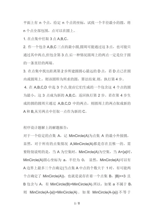
平面上有n个点，给定n个点的坐标，试找一个半径最小的圆，将n 个点全部包围，点可以在圆上。

1. 在点集中任取3点A,B,C。

2. 作一个包含A,B,C三点的最小圆,圆周可能通过这3点，也可能只通过其中两点,但包含第3点.后一种情况圆周上的两点一定是位于圆的一条直径的两端。

3. 在点集中找出距离第2步所建圆圆心最远的D点，若D点已在圆内或圆周上，则该圆即为所求的圆，算法结束.则，执行第4步。

4. 在A,B,C,D中选3个点,使由它们生成的一个包含这4个点的圆为最小，这3 点成为新的A,B,C，返回执行第2步。

若在第4步生成的圆的圆周只通过A,B,C,D 中的两点，则圆周上的两点取成新的A和B,从另两点中任取一点作为新的C。

程序设计题解上的解题报告：对于一个给定的点集A，记MinCircle(A)为点集A的最小外接圆，显然，对于所有的点集情况A,MinCircle(A)都是存在且惟一的。

需要特别说明的是，当A为空集时，MinCircle(A)为空集，当A={a}时，MinCircle(A)圆心坐标为a，半径为0；显然，MinCircle(A)可以有A边界上最多三个点确定(当点集A中点的个数大于1时，有可能两个点确定了MinCircle(A))，也就是说存在着一个点集B，|B|<=3 且B包含与A，有MinCircle(B)=MinCircle(A).所以，如果a不属于B，则MinCircle(A-{a})=MinCircle(A)。

如果MinCircle(A-{a})不等于MinCircle(A),则a属于B。

所以我们可以从一个空集R开始，不断的把题目中给定的点集中的点加入R，同时维护R的外接圆最小，这样就可以得到解决该题的算法。

不断添加圆，维护最小圆。

如果添加的点i在圆内，不动，否则：问题转化为求1~I的最小圆：求出1与I的最小圆，并且扫描j=2~I-1，维护（1）+（i）+(2~j)的最小圆，如果找到J不在最小圆内，问题转化为：求(1~J)+(i)的最小圆。

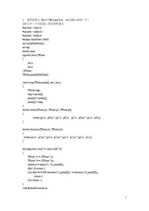
1.扇形的重心Xc = 2*R*sinA/3/A （A为圆心角的一半）2.N点中三个点组成三角形面积最大#include <stdio.h>#include <stdlib.h>#include <math.h>#define MaxNode 50005int stack[MaxNode];int top;double max;typedef struct TPoint{int x;int y;}TPoint;TPoint point[MaxNode];void swap(TPoint point[], int i, int j){TPoint tmp;tmp = point[i];point[i] = point[j];point[j] = tmp;}double multi(TPoint p1, TPoint p2, TPoint p0){return (p1.x - p0.x) * (p2.y - p0.y) - (p2.x - p0.x) * (p1.y - p0.y); }double distance(TPoint p1, TPoint p2){return (p1.x - p2.x) * (p1.x - p2.x) + (p1.y - p2.y) * (p1.y - p2.y);}int cmp(const void *a, const void *b){TPoint *c = (TPoint *)a;TPoint *d = (TPoint *)b;double k = multi(*c, *d, point[0]);if(k< 0) return 1;else if(k == 0 && distance(*c, point[0]) >= distance(*d, point[0])) return 1;else return -1;}void grahamScan(int n){//Graham扫描求凸包int i, u;//将最左下的点调整到p[0]的位置u = 0;for(i = 1;i <= n - 1;i++){if((point[i].y < point[u].y) ||(point[i].y == point[u].y && point[i].x < point[u].x)) u = i;}swap(point, 0, u);//将平p[1]到p[n - 1]按按极角排序，可采用快速排序qsort(point + 1, n - 1, sizeof(point[0]), cmp);for(i = 0;i <= 2;i++) stack[i] = i;top = 2;for(i = 3;i <= n - 1;i++){while(multi(point[i], point[stack[top]], point[stack[top - 1]]) >= 0){ top--;if(top == 0) break;}top++;stack[top] = i;}}int main(){double triangleArea(int i, int j, int k);void PloygonTriangle();int i, n;while(scanf("%d", &n) && n != -1){for(i = 0;i < n;i++)scanf("%d%d", &point[i].x, &point[i].y);if(n <= 2){printf("0.00\n");continue;}if(n == 3){printf("%.2lf\n", triangleArea(0, 1, 2));continue;}grahamScan(n);PloygonTriangle();printf("%.2lf\n", max);}return 0;}void PloygonTriangle(){double triangleArea(int i, int j, int k);int i, j , k;double area, area1;max = -1;for(i = 0;i <= top - 2;i++){k = -1;for(j = i + 1; j <= top - 1;j++){if(k <= j) k= j + 1;area = triangleArea(stack[i], stack[j], stack[k]);if(area > max) max = area;while(k + 1 <= top){area1= triangleArea(stack[i], stack[j], stack[k + 1]);if(area1 < area) break;if(area1 > max) max = area1;area = area1;k++;}}}}double triangleArea(int i, int j, int k){//已知三角形三个顶点的坐标，求三角形的面积double l = fabs(point[i].x * point[j].y + point[j].x * point[k].y + point[k].x * point[i].y - point[j].x * point[i].y- point[k].x * point[j].y - point[i].x * point[k].y) / 2;return l;}3.N个点最多组成多少个正方形#include<stdio.h>#include<stdlib.h>#include<math.h>#define eps 1e-6#define pi acos(-1.0)#define PRIME 9991struct point{int x, y;}p[2201];int n;struct HASH{int cnt;int next;}hash[50000];int hashl;int Hash(int n){int i = n % PRIME;while(hash[i].next != -1){if(hash[hash[i].next].cnt == n) return 1;else if(hash[hash[i].next].cnt > n) break;i = hash[i].next;}hash[hashl].cnt = n;hash[hashl].next = hash[i].next;hash[i].next = hashl;hashl++;return 0;}int Hash2(int n){int i = n % PRIME;while(hash[i].next != -1){if(hash[hash[i].next].cnt == n) return 1;else if(hash[hash[i].next].cnt > n) return 0;i = hash[i].next;}return 0;}int check(double ax, double ay, int &x, int &y){int a0 = (int)ax;int b0 = (int)ay;int tag1 = 0, tag2 = 0;if(fabs(a0 - ax) < eps){tag1 = 1;x = a0;}else if(fabs(a0 + 1 - ax) < eps){tag1 = 1;x = a0 + 1;}if(fabs(b0 - ay) < eps){tag2 = 1;y = b0;}else if(fabs(b0 + 1 - ay) < eps){y = b0 + 1;tag2 = 1;}if(tag1 == 1 && tag2 == 1) return 1;else return 0;}int squares(point p1, point p2, point &p3, point &p4) {double a = (double)p2.x - p1.x;double b = (double)p2.y - p1.y;double midx = ((double)p1.x + p2.x) / 2;double midy = ((double)p1.y + p2.y) / 2;double tmp = a * a + b * b;double x1 = sqrt(b * b) / 2;double y1;if(fabs(b) < eps) y1 = sqrt(a * a + b * b) / 2;else y1 = -a * x1 / b;x1 += midx;y1 += midy;if(check(x1, y1, p3.x, p3.y) == 0) return 0;x1 = 2 * midx - x1;y1 = 2 * midy - y1;if(check(x1, y1, p4.x, p4.y) == 0) return 0;return 1;}int main(){int i, j, cnt;while(scanf("%d", &n) != EOF && n){for(i = 0;i < PRIME;i++) hash[i].next = -1;hashl = PRIME;int x1, y1, x2, y2;for (i = 0; i < n; i++){scanf("%d%d", &p[i].x, &p[i].y);Hash((p[i].x + 100000) * 100000 + p[i].y + 100000);}cnt = 0;for (i = 0; i < n; i++){for (j = i + 1; j < n; j++){point a, b;if(squares(p[i], p[j], a, b) == 0) continue;if(Hash2((a.x + 100000) * 100000 + a.y + 100000) == 0) continue;if(Hash2((b.x + 100000) * 100000 + b.y + 100000) == 0) continue;cnt++;}}printf("%d\n", cnt / 2);}return 0;}4.单位圆覆盖最多点/*平面上N个点，用一个半径R的圆去覆盖，最多能覆盖多少个点？比较经典的题目。

最小圆覆盖算法摘要：1.最小圆覆盖算法的定义2.最小圆覆盖算法的应用场景3.最小圆覆盖算法的基本原理4.最小圆覆盖算法的求解方法5.最小圆覆盖算法的优缺点正文：1.最小圆覆盖算法的定义最小圆覆盖算法是一种计算几何算法，它的目标是在一个平面上找到一个最小的圆，使得这个圆能够覆盖给定的一组点集。

这个算法在许多实际应用场景中有着广泛的应用，例如在无线通信、数据挖掘和机器人路径规划等领域。

2.最小圆覆盖算法的应用场景最小圆覆盖算法在许多实际应用场景中有着广泛的应用，例如在无线通信、数据挖掘和机器人路径规划等领域。

在无线通信中，该算法可以应用于基站的位置选择，使得覆盖范围最大化，同时保证最小的信号干扰。

在数据挖掘中，最小圆覆盖算法可以用于聚类分析，将数据点分为若干个类别。

在机器人路径规划中，最小圆覆盖算法可以帮助机器人找到一个最优路径，使得它能够覆盖所有需要清洁或者巡逻的区域。

3.最小圆覆盖算法的基本原理最小圆覆盖算法的基本原理是：对于给定的一组点集，我们可以通过计算这些点到某个点的距离，找到一个最小的圆，使得这个圆的半径最大，同时保证这个圆能够覆盖所有的点。

4.最小圆覆盖算法的求解方法最小圆覆盖算法的求解方法有很多，其中比较常见的有以下几种：- 贪心算法：贪心算法是一种简单的启发式算法，它通过每次选择一个距离当前点最近的点，不断扩大圆的半径，直到所有的点都被覆盖。

贪心算法的时间复杂度为O(n)，其中n 为点集的规模。

- 圆锥算法：圆锥算法是一种基于几何特征的算法，它通过计算点集中每个点到某个点的距离，找到一个最小的圆锥，使得这个圆锥的底面圆能够覆盖所有的点。

圆锥算法的时间复杂度为O(nlogn)。

- 蚁群算法：蚁群算法是一种基于自然界生物智能的算法，它通过模拟蚂蚁觅食过程中的信息素更新机制，逐步寻找到一个最小的圆。

蚁群算法的时间复杂度为O(n^2)。

5.最小圆覆盖算法的优缺点最小圆覆盖算法的优点是求解速度快，尤其是对于规模较小的点集，贪心算法和圆锥算法都能够在较短的时间内找到一个合适的解。

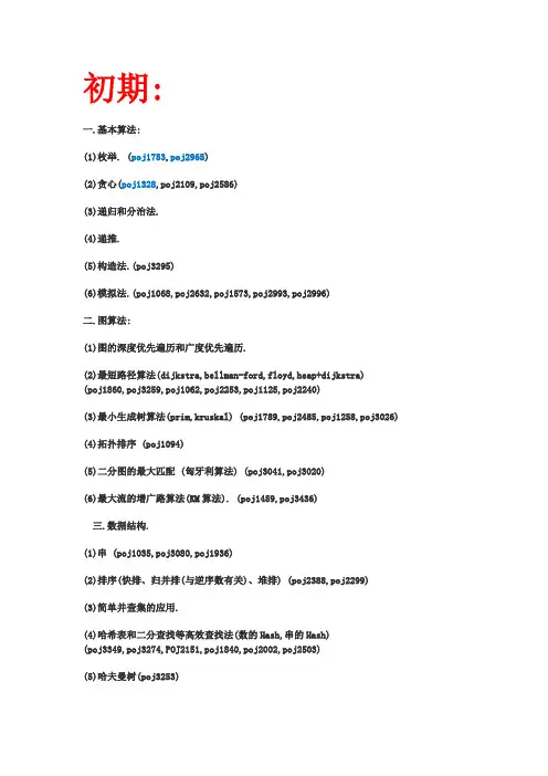
初期:一.基本算法:(1)枚举. (poj1753,poj2965)(2)贪心(poj1328,poj2109,poj2586)(3)递归和分治法.(4)递推.(5)构造法.(poj3295)(6)模拟法.(poj1068,poj2632,poj1573,poj2993,poj2996)二.图算法:(1)图的深度优先遍历和广度优先遍历.(2)最短路径算法(dijkstra,bellman-ford,floyd,heap+dijkstra)(poj1860,poj3259,poj1062,poj2253,poj1125,poj2240)(3)最小生成树算法(prim,kruskal) (poj1789,poj2485,poj1258,poj3026)(4)拓扑排序 (poj1094)(5)二分图的最大匹配 (匈牙利算法) (poj3041,poj3020)(6)最大流的增广路算法(KM算法). (poj1459,poj3436)三.数据结构.(1)串 (poj1035,poj3080,poj1936)(2)排序(快排、归并排(与逆序数有关)、堆排) (poj2388,poj2299)(3)简单并查集的应用.(4)哈希表和二分查找等高效查找法(数的Hash,串的Hash)(poj3349,poj3274,POJ2151,poj1840,poj2002,poj2503)(5)哈夫曼树(poj3253)(6)堆(7)trie树(静态建树、动态建树) (poj2513)四.简单搜索(1)深度优先搜索 (poj2488,poj3083,poj3009,poj1321,poj2251)(2)广度优先搜索(poj3278,poj1426,poj3126,poj3087.poj3414)(3)简单搜索技巧和剪枝(poj2531,poj1416,poj2676,1129)五.动态规划(1)背包问题. (poj1837,poj1276)(2)型如下表的简单DP(可参考lrj的书 page149):1.E[j]=opt{D+w(i,j)} (poj3267,poj1836,poj1260,poj2533)2.E[i,j]=opt{D[i-1,j]+xi,D[i,j-1]+yj,D[i-1][j-1]+zij} (最长公共子序列) (poj3176,poj1080,poj1159)3.C[i,j]=w[i,j]+opt{C[i,k-1]+C[k,j]}.(最优二分检索树问题)六.数学(1)组合数学:1.加法原理和乘法原理.2.排列组合.3.递推关系.(POJ3252,poj1850,poj1019,poj1942)(2)数论.1.素数与整除问题2.进制位.3.同余模运算.(poj2635, poj3292,poj1845,poj2115)(3)计算方法.1.二分法求解单调函数相关知识.(poj3273,poj3258,poj1905,poj3122)七.计算几何学.(1)几何公式.(2)叉积和点积的运用(如线段相交的判定,点到线段的距离等). (poj2031,poj1039)(3)多边型的简单算法(求面积)和相关判定(点在多边型内,多边型是否相交)(poj1408,poj1584)(4)凸包. (poj2187,poj1113)中级:一.基本算法:(1)C++的标准模版库的应用. (poj3096,poj3007)(2)较为复杂的模拟题的训练(poj3393,poj1472,poj3371,poj1027,poj2706)二.图算法:(1)差分约束系统的建立和求解. (poj1201,poj2983)(2)最小费用最大流(poj2516,poj2516,poj2195)(3)双连通分量(poj2942)(4)强连通分支及其缩点.(poj2186)(5)图的割边和割点(poj3352)(6)最小割模型、网络流规约(poj3308, )三.数据结构.(1)线段树. (poj2528,poj2828,poj2777,poj2886,poj2750)(2)静态二叉检索树. (poj2482,poj2352)(3)树状树组(poj1195,poj3321)(4)RMQ. (poj3264,poj3368)(5)并查集的高级应用. (poj1703,2492)(6)KMP算法. (poj1961,poj2406)四.搜索(1)最优化剪枝和可行性剪枝(2)搜索的技巧和优化 (poj3411,poj1724)(3)记忆化搜索(poj3373,poj1691)五.动态规划(1)较为复杂的动态规划(如动态规划解特别的施行商问题等) (poj1191,poj1054,poj3280,poj2029,poj2948,poj1925,poj3034)(2)记录状态的动态规划. (POJ3254,poj2411,poj1185)(3)树型动态规划(poj2057,poj1947,poj2486,poj3140)六.数学(1)组合数学:1.容斥原理.2.抽屉原理.3.置换群与Polya定理(poj1286,poj2409,poj3270,poj1026).4.递推关系和母函数.(2)数学.1.高斯消元法(poj2947,poj1487, poj2065,poj1166,poj1222)2.概率问题. (poj3071,poj3440)3.GCD、扩展的欧几里德(中国剩余定理) (poj3101)(3)计算方法.1.0/1分数规划. (poj2976)2.三分法求解单峰(单谷)的极值.3.矩阵法(poj3150,poj3422,poj3070)4.迭代逼近(poj3301)(4)随机化算法(poj3318,poj2454)(5)杂题. (poj1870,poj3296,poj3286,poj1095)七.计算几何学.(1)坐标离散化.(2)扫描线算法(例如求矩形的面积和周长并,常和线段树或堆一起使用).(poj1765,poj1177,poj1151,poj3277,poj2280,poj3004)(3)多边形的内核(半平面交)(poj3130,poj3335)(4)几何工具的综合应用.(poj1819,poj1066,poj2043,poj3227,poj2165,poj3429)高级:一.基本算法要求:(1)代码快速写成,精简但不失风格(poj2525,poj1684,poj1421,poj1048,poj2050,poj3306)(2)保证正确性和高效性. poj3434二.图算法:(1)度限制最小生成树和第K最短路. (poj1639)(2)最短路,最小生成树,二分图,最大流问题的相关理论(主要是模型建立和求解) (poj3155, poj2112,poj1966,poj3281,poj1087,poj2289,poj3216,poj2446) (3)最优比率生成树. (poj2728)(4)最小树形图(poj3164)(5)次小生成树.(6)无向图、有向图的最小环三.数据结构.(1)trie图的建立和应用. (poj2778)(2)LCA和RMQ问题(LCA(最近公共祖先问题) 有离线算法(并查集+dfs) 和在线算法(RMQ+dfs)).(poj1330)(3)双端队列和它的应用(维护一个单调的队列,常常在动态规划中起到优化状态转移的目的).(poj2823)(4)左偏树(可合并堆).(5)后缀树(非常有用的数据结构,也是赛区考题的热点). (poj3415,poj3294)四.搜索(1)较麻烦的搜索题目训练(poj1069,poj3322,poj1475,poj1924,poj2049,poj3426)(2)广搜的状态优化:利用M进制数存储状态、转化为串用hash表判重、按位压缩存储状态、双向广搜、A*算法. (poj1768,poj1184,poj1872,poj1324,poj2046,poj1482)(3)深搜的优化:尽量用位运算、一定要加剪枝、函数参数尽可能少、层数不易过大、可以考虑双向搜索或者是轮换搜索、IDA*算法.(poj3131,poj2870,poj2286)五.动态规划(1)需要用数据结构优化的动态规划. (poj2754,poj3378,poj3017)(2)四边形不等式理论.(3)较难的状态DP(poj3133)六.数学(1)组合数学.1.MoBius反演(poj2888,poj2154)2.偏序关系理论.(2)博奕论.1.极大极小过程(poj3317,poj1085)2.Nim问题.七.计算几何学.(1)半平面求交(poj3384,poj2540)(2)可视图的建立(poj2966)(3)点集最小圆覆盖.(4)对踵点(poj2079)八.综合题.(poj3109,poj1478,poj1462,poj2729,poj2048,poj3336,poj3315,poj2148,poj1263) 以及补充Dp状态设计与方程总结1.不完全状态记录<1>青蛙过河问题<2>利用区间dp2.背包类问题<1> 0-1背包，经典问题<2>无限背包，经典问题<3>判定性背包问题<4>带附属关系的背包问题<5> + -1背包问题<6>双背包求最优值<7>构造三角形问题<8>带上下界限制的背包问题(012背包)3.线性的动态规划问题<1>积木游戏问题<2>决斗（判定性问题）<3>圆的最大多边形问题<4>统计单词个数问题<5>棋盘分割<6>日程安排问题<7>最小逼近问题(求出两数之比最接近某数/两数之和等于某数等等)<8>方块消除游戏(某区间可以连续消去求最大效益)<9>资源分配问题<10>数字三角形问题<11>漂亮的打印<12>邮局问题与构造答案<13>最高积木问题<14>两段连续和最大<15>2次幂和问题<16>N个数的最大M段子段和<17>交叉最大数问题4.判定性问题的dp(如判定整除、判定可达性等)<1>模K问题的dp<2>特殊的模K问题，求最大(最小)模K的数<3>变换数问题5.单调性优化的动态规划<1>1-SUM问题<2>2-SUM问题<3>序列划分问题(单调队列优化)6.剖分问题(多边形剖分/石子合并/圆的剖分/乘积最大)<1>凸多边形的三角剖分问题<2>乘积最大问题<3>多边形游戏(多边形边上是操作符,顶点有权值)<4>石子合并(N^3/N^2/NLogN各种优化)7.贪心的动态规划<1>最优装载问题<2>部分背包问题<3>乘船问题<4>贪心策略<5>双机调度问题Johnson算法8.状态dp<1>牛仔射击问题(博弈类)<2>哈密顿路径的状态dp<3>两支点天平平衡问题<4>一个有向图的最接近二部图9.树型dp<1>完美服务器问题(每个节点有3种状态)<2>小胖守皇宫问题<3>网络收费问题<4>树中漫游问题<5>树上的博弈<6>树的最大独立集问题<7>树的最大平衡值问题<8>构造树的最小环转一个搞ACM需要的掌握的算法.要注意,ACM的竞赛性强,因此自己应该和自己的实际应用联系起来.适合自己的才是好的,有的人不适合搞算法,喜欢系统架构,因此不要看到别人什么就眼红, 发挥自己的长处,这才是重要的.第一阶段：练经典常用算法，下面的每个算法给我打上十到二十遍，同时自己精简代码，因为太常用，所以要练到写时不用想，10-15分钟内打完，甚至关掉显示器都可以把程序打出来.1.最短路(Floyd、Dijstra,BellmanFord)2.最小生成树(先写个prim,kruscal要用并查集，不好写)3.大数（高精度）加减乘除4.二分查找. (代码可在五行以内)5.叉乘、判线段相交、然后写个凸包.6.BFS、DFS,同时熟练hash表(要熟，要灵活,代码要简)7.数学上的有：辗转相除（两行内），线段交点、多角形面积公式.8. 调用系统的qsort, 技巧很多，慢慢掌握.9. 任意进制间的转换第二阶段：练习复杂一点，但也较常用的算法。

ACM主要算法介绍初期篇一、基本算法(1)枚举(poj1753, poj2965)(2)贪心(poj1328, poj2109, poj2586)(3)递归和分治法(4)递推(5)构造法(poj3295)(6)模拟法(poj1068, poj2632, poj1573, poj2993, poj2996)二、图算法(1)图的深度优先遍历和广度优先遍历(2)最短路径算法(dijkstra, bellman-ford, floyd, heap+dijkstra)(poj1860, poj3259, poj1062, poj2253, poj1125, poj2240)(3)最小生成树算法(prim, kruskal)(poj1789, poj2485, poj1258, poj3026)(4)拓扑排序(poj1094)(5)二分图的最大匹配(匈牙利算法)(poj3041, poj3020)(6)最大流的增广路算法(KM算法)(poj1459, poj3436)三、数据结构(1)串(poj1035, poj3080, poj1936)(2)排序(快排、归并排(与逆序数有关)、堆排)(poj2388, poj2299)(3)简单并查集的应用(4)哈希表和二分查找等高效查找法(数的Hash, 串的Hash)(poj3349, poj3274, POJ2151, poj1840, poj2002, poj2503)(5)哈夫曼树(poj3253)(6)堆(7)trie树(静态建树、动态建树)(poj2513)四、简单搜索(1)深度优先搜索(poj2488, poj3083, poj3009, poj1321, poj2251)(2)广度优先搜索(poj3278, poj1426, poj3126, poj3087, poj3414)(3)简单搜索技巧和剪枝(poj2531, poj1416, poj2676, 1129)五、动态规划(1)背包问题(poj1837, poj1276)(2)型如下表的简单DP(可参考lrj的书page149)：1.E[j]=opt{D+w(i,j)} (poj3267, poj1836, poj1260, poj2533)2.E[i,j]=opt{D[i-1,j]+xi,D[i,j-1]+yj,D[i-1][j-1]+zij} (最长公共子序列)(poj3176, poj1080, poj1159)3.C[i,j]=w[i,j]+opt{C[i,k-1]+C[k,j]} (最优二分检索树问题)六、数学(1)组合数学1.加法原理和乘法原理2.排列组合3.递推关系(poj3252, poj1850, poj1019, poj1942)(2)数论1.素数与整除问题2.进制位3.同余模运算(poj2635, poj3292, poj1845, poj2115)(3)计算方法1.二分法求解单调函数相关知识(poj3273, poj3258, poj1905, poj3122)七、计算几何学(1)几何公式(2)叉积和点积的运用(如线段相交的判定，点到线段的距离等)(poj2031, poj1039)(3)多边型的简单算法(求面积)和相关判定(点在多边型内，多边型是否相交)(poj1408, poj1584)(4)凸包(poj2187, poj1113)中级篇一、基本算法(1)C++的标准模版库的应用(poj3096, poj3007)(2)较为复杂的模拟题的训练(poj3393, poj1472, poj3371, poj1027,poj2706)二、图算法(1)差分约束系统的建立和求解(poj1201, poj2983)(2)最小费用最大流(poj2516, poj2195)(3)双连通分量(poj2942)(4)强连通分支及其缩点(poj2186)(5)图的割边和割点(poj3352)(6)最小割模型、网络流规约(poj3308)三、数据结构(1)线段树(poj2528, poj2828, poj2777, poj2886, poj2750)(2)静态二叉检索树(poj2482, poj2352)(3)树状树组(poj1195, poj3321)(4)RMQ(poj3264, poj3368)(5)并查集的高级应用(poj1703, 2492)(6)KMP算法(poj1961, poj2406)四、搜索(1)最优化剪枝和可行性剪枝(2)搜索的技巧和优化(poj3411, poj1724)(3)记忆化搜索(poj3373, poj1691)五、动态规划(1)较为复杂的动态规划(如动态规划解特别的施行商问题等)(poj1191, poj1054, poj3280, poj2029, poj2948, poj1925, poj3034)(2)记录状态的动态规划(poj3254, poj2411, poj1185)(3)树型动态规划(poj2057, poj1947, poj2486, poj3140)六、数学(1)组合数学1.容斥原理2.抽屉原理3.置换群与Polya定理(poj1286, poj2409, poj3270, poj1026)4.递推关系和母函数(2)数学1.高斯消元法(poj2947, poj1487, poj2065, poj1166, poj1222)2.概率问题(poj3071, poj3440)3.GCD、扩展的欧几里德(中国剩余定理)(poj3101)(3)计算方法1.0/1分数规划(poj2976)2.三分法求解单峰(单谷)的极值3.矩阵法(poj3150, poj3422, poj3070)4.迭代逼近(poj3301)(4)随机化算法(poj3318, poj2454)(5)杂题(poj1870, poj3296, poj3286, poj1095)七、计算几何学(1)坐标离散化(2)扫描线算法(例如求矩形的面积和周长，并常和线段树或堆一起使用)(poj1765, poj1177, poj1151, poj3277, poj2280, poj3004)(3)多边形的内核(半平面交)(poj3130, poj3335)(4)几何工具的综合应用(poj1819, poj1066, poj2043, poj3227, poj2165, poj3429)高级篇一、基本算法要求(1)代码快速写成，精简但不失风格(poj2525, poj1684, poj1421,poj1048, poj2050, poj3306)(2)保证正确性和高效性(poj3434)二、图算法(1)度限制最小生成树和第K最短路(poj1639)(2)最短路，最小生成树，二分图，最大流问题的相关理论(主要是模型建立和求解)(poj3155, poj2112, poj1966, poj3281, poj1087, poj2289, poj3216, poj2446)(3)最优比率生成树(poj2728)(4)最小树形图(poj3164)(5)次小生成树(6)无向图、有向图的最小环三、数据结构(1)trie图的建立和应用(poj2778)(2)LCA和RMQ问题(LCA(最近公共祖先问题)，有离线算法(并查集+dfs)和在线算法(RMQ+dfs))(poj1330)(3)双端队列和它的应用(维护一个单调的队列，常常在动态规划中起到优化状态转移的目的)(poj2823)(4)左偏树(可合并堆)(5)后缀树(非常有用的数据结构，也是赛区考题的热点)(poj3415,poj3294)四、搜索(1)较麻烦的搜索题目训练(poj1069, poj3322, poj1475, poj1924,poj2049, poj3426)(2)广搜的状态优化：利用M进制数存储状态、转化为串用hash表判重、按位压缩存储状态、双向广搜、A*算法(poj1768, poj1184, poj1872, poj1324, poj2046, poj1482)(3)深搜的优化：尽量用位运算、一定要加剪枝、函数参数尽可能少、层数不易过大、可以考虑双向搜索或者是轮换搜索、IDA*算法(poj3131, poj2870, poj2286)五、动态规划(1)需要用数据结构优化的动态规划(poj2754, poj3378, poj3017)(2)四边形不等式理论(3)较难的状态DP(poj3133)六、数学(1)组合数学1.MoBius反演(poj2888, poj2154)2.偏序关系理论(2)博奕论1.极大极小过程(poj3317, poj1085)2.Nim问题七、计算几何学(1)半平面求交(poj3384, poj2540)(2)可视图的建立(poj2966)(3)点集最小圆覆盖(4)对踵点(poj2079)八、综合题(poj3109, poj1478, poj1462, poj2729, poj2048, poj3336, poj3315, poj2148, poj1263)附录：POJ是“北京大学程序在线评测系统”（Peking University Online Judge）的缩写，是个提供编程题目的网站，兼容Pascal、C、C＋＋、Java、Fortran等多种语言。

最小顶点覆盖算法
最小顶点覆盖算法是指在一个给定的有向图或者无向图中，找出最小的顶点集合，使
得每一条边都至少与其中的一个顶点相邻接。

在实际应用中，最小顶点覆盖算法在寻找最
小链覆盖、图染色等问题中有重要的作用。

最小顶点覆盖算法的基本思想是把顶点覆盖转换成最大匹配问题，然后使用网络流算
法来求解。

最大匹配是指在一个二分图中，选出最多的两两不相邻的边，使得这些边两端
都没有被选中。

如果将一个图的最大匹配个数记为M，则该图的最小顶点覆盖个数就是N-M，其中N为图中的顶点数。

具体实现中，我们首先将一个无向图G转化为一个二分图B，然后将B的匹配边集合（即将两个集合中的点匹配的边的集合）转化成顶点覆盖集合。

这个转化的过程可以使用
König氏定理来完成。

König氏定理是一个非常重要的结论，它给出了二分图中最小顶点覆盖与最大匹配的关系，即最小顶点覆盖=最大匹配。

具体实现时，我们使用匈牙利算法来求解最大匹配，该算法是一个经典的图论算法，
它使用增广路的思想，将匹配边不断扩大，从而达到最大值。

然后使用König氏定理将最
大匹配边集合转化成最小顶点覆盖集合。

最小顶点覆盖算法的时间复杂度为O(V^3)，其中V为顶点个数。

虽然该算法时间复杂度较高，但是在实际应用中，由于它的准确性和有效性，被广泛地应用于图论相关领域。

同时，最小顶点覆盖算法也是一种十分优秀的解决方案，能够为我们在实际应用中遇到的
各种问题提供较好的指导和帮助。

逼近4正则图的最小顶点覆盖问题的难解性陈文彬【摘要】证明了逼近4正则图的最小顶点覆盖问题在某个常数因子内是计算难解的.相似地,对于5正则图、6正则图等的最小顶点覆盖问题,这个结论也成立.已知逼近3正则图的最小顶点覆盖问题在某个常数因子内是计算难解的,文章扩展了这个结果到4正则图情况,用K-归约证明这个结果,给出了一个从3正则图的最小顶点覆盖问题到4正则图的最小顶点覆盖问题的K-归约.【期刊名称】《广州大学学报（自然科学版）》【年(卷),期】2014(013)001【总页数】5页(P65-69)【关键词】NP-难解性;计算复杂性;正则图;顶点覆盖;近似性【作者】陈文彬【作者单位】广州大学计算机科学与教育软件学院,广东广州510006【正文语种】中文【中图分类】TP301.50 IntroductionIn computational complexity，researchers have found a great deal of combinational optimization problems that are computationally hard.The intractability of combinational optimization problems motivatesresearchers to find approximation algorithms solving them.In practice，formany combinational optimization problems，it is hard to design efficient approximation algorithms.Because the theory of NP-completeness ［1-3］ can classify the hardness of combinational optimization problems，researchers strive to study the complexity of approximation algorithms ［4］.Gradually，the complexity study of approximation algorithms of NP-complete optimization problems becomes a very active area of research.With the development of the research field，researchers find that there are four classes of computational problems for the hardness of approximation［5］.For many problems，researchers can design approximation algorithms.For other problems，such as Set Cover，no constant factor approximation algorithms exist under the conjureP≠NP.Other problems like Clique are harder to approximate.In fact，few inapproximability results were known before 1990.Until 1990，FEIGE，et al.found that probabilistic proof systems can be used to prove hardness of approximation［6］.After that，the PCP theorem was discovered by ARORA，et al［7-9］.Using the PCP theorem，they showed that approximating the MAX 3SAT within some constant factor is NP-hard.Under the L-reduction of Ref.［10］，inapproximability results for several other problems were proven.For an undirected graph G=(V，E)，a vertex cover is a subset V′⊆V such that，for each edge(u，v)∈E，at least one of u and v belongs to V′.It is well known that the problem of finding a minimum size vertex cover is NP-hard.Under Unique Game Conjecture，KHOT，et al.proved that it is NP-hard to approximate the vertex cover problem within 2- ε for any ε ＞ 0［11］.DINUR，et al.showed that approximating the vertex cover problem is NP-hard within a factor 1.36［12］.AUSRIN，etal.study the inapproxi mability of vertex cover in bounded degree graphs.They showed that the vertex cover problem in a bounded degree d graph is Unique Game-hard to approximate to within a factorAfter PCP theorem was discovered，the hardness of approximating MAX 3SAT-d was proven.The L-reduction from MAX 3SAT-d to Vertex Cover for bounded degree graphs was given in Ref.［14］，which proved the hardness of approximating the Minimum Vertex Cover Problem for bounded degree graphs within some constant factor.Furthermore，in Ref.［14］，the hardness of approximating the Minimum Vertex Cover Problem for 3-regular graphs within some constant factor was proven using an L-reduction from bounded 3-degree graphs to 3-regular graphs.In their L-reduction，they constructed an extra graph H and connected 1-degree vertices and 2-degree vertices of a bounded 3-degree graph G to the 2-degree vertices of H，then the graph G was transformed to a 3-regular graph.Furthermore，it was proven that the transformation satisfied the conditions of L-reduction.But they neglect a special situation:when a bounded 3-degree graph G has only one 2-degree vertex and other vertices are 3-degree vertices，the constructed extra graph H has two edges connecting the same two vertices.Hence the graph H is nota simple graph.So in this situation，the transformation is not correct.In this paper，we first correct the error mentioned above.In order to correct that error，we construct a new graph H′instead of H.The new graph H′has one 2-degree vertex and four 3-degree vertices，which is simpler than H.In order to transform a bounded 3-degree graph G to a 3-regular graph G′，we connect its every 1-degree vertex to the 2-degree vertices of two graphs H′and conn ect its every 2-degree vertex to the 1-degree vertex of one graph H′.Second，We can extend our method to prove the hardness of approximating the Minimum Vertex Cover Problem for 4-regular graphs.We give a K-reduction from 3 regular graphs to 4 regular graphs.Thus，we get that approximating the Minimum Vertex Cover Problem for 4-regular graphs within some constant factor is NP-hard.Similarly，approximating the Minimum Vertex Cover Problem for k-regular(k＞4)graphswithin some constant factor is NP-hard.1 Prelim inariesIn the following，we introduce some definitions and known facts.Some reductions preserving approximation within constants has been proposed，such as L-deductions［10］，gap-preserving reductions［5］.Because a K-reduction is easier than an L-reduction in some situation，we use the K-reduction in this paper.We first give the definition of K reduction. Definition 1［15］LetΠ and Γ be twominimization(maximization)optimization problems.We say thatΠK-reducesΓif there are two polynomialtime algorithms f，g，and constantsα，β ＞0 such that for every instance IofΠ:(K1)Algorithm f produces an instance f(I)of Γ，such that the optima of Iandf(I)，OPT(I)and OPT(f(I))respectively，satisfy OPT(f(I))≤α·OPT(I).(K2)Given any solution y ofΓ with cost c′，algorithm g produces a solution g(y)of I with cost c such that c≤βc′The following two propositions have been proven in Ref.［15］.Lemma 1 IfΠK-reducesΓandΓK-reduces Γ′，Π K-reducesΓ′.Lemma 2 IfΠ K-reducesΓ (where，bothΠ andΓare eithermaxi mization problems ormini mization problems)，and there is a polynomial-time approximation algorithm forΓ with performance ratio r，then there is a polynomial-time approximation algorithm forΠ with performance ratio αβr.In order to prove our result，we now quote one theorem coming from Ref.［14］.Lemma 3 (Theorem 11.15 in Ref.［14］)There is a r＞1 such that finding r-approximations to the Minimum Vertex Cover for bounded k-degree(k≥3)graphs is NP-hard.2 The hardness of approximating the M inimum Vertex Cover for 4-regular graphsIn this section，we first prove that approximating the Minimum Vertex Cover for 3-regular graphs within some constant factor is hard.Although the conclusion has been proven in Ref.［14］，there is an error mentioned in section 1.We correct the error.The reduction which was used in their proof is an L-reduction.In our proof，we use a K-reduction instead of an L-reduction.We give a K-reduction from bounded 3-degree graphs to 3-regular graphs.Theorem 1 There is a r＞1 such that finding r-approximations to the Minimum Vertex Cover for 3-regular graphs is NP-hard.Proof We give a K-reduction from bounded 3-degree graphs to 3-regular graphs.Let graph G be an instance of bounded 3-degree graphs.We assume that G has i1-degree vertices and j2-degree vertices.We c onstruct a graph H′which has one 2-degree vertex and four 3-degree vertices as Fig.1.Fig.1 An instance of graph H′We need construct(2i+j)graphs H′.And then，we connect every 1-degree vertex of G to two 2-degree vertices of two graphs H′and connect ever y 2-degree vertex of G to the 2-degree vertex of a graph H′.So we get a 3-regular graph G′.We notice that the Minimum Vertex Cover of a graph H′includes three vertices.So OPT(G′)=OPT(G)+3(2i+j).Because the graph G has at least(i+2j)/2 edges and its every vertex covers atmost three edges，3·OPT(G)≥(i+2j)/2.So OPT(G)≥(i+2j)/6.Hence，2i+j≤12·OPT(G).Hence，OPT(G′)≤37·OPT(G).So we verify that the reduction satisfies the condition(K1).Suppose C′is a Vertex Cover of graph G′.Deleting the vertices that belong to th ose graphs H′，we get a vertices set C that is a vertex cover of the graph G.Because C⊆C′，|C|≤ |C′|.So we verify that the reduction satisfies the condition(K2).According to Lemma 2 and Lemma 3，we conclude that there is a r＞1 such that finding r-approximations to the Minimum Vertex Cover for 3-regular graphs is NP-hard.In order to prove the hardness of approximating the Minimum VertexCover for 4-regular graphs，we give a K-reduction from 3-regular graphs to 4-regular graphs.Theorem 2 There is a r＞1 such that finding r-approximations to the Minimum Vertex Cover for 4-regular graphs is NP-hard.Proof We give a K-reduction from 3-regular graphs to 4-regular graphs.Let G1，an instance of3-regular graphs，has n vertices.G2 is a copy of G1.Connecting every vertex of G1 to its copy vertex of G2，we get a 4-regular graph G′.For example(Fig.2):Fig.2 An instance of a 3-regular graph G1 is reduced to a 4-regular graph G′Obviously，a vertex cover of G1 and all vertices of G2 is a vertex cover of G′.So OPT(G′)≤OPT(G1)+n.Because G1 has3n/2 edges and every vertex covers three edges，3·OPT(G1)≥3n/2.So n≤2·OPT(G1).Hence，So we verify that the reduction satisfies the condition(K1).Suppose C′is a Vertex Cover of graph G′.Deleting the vertices that belong to the graph G2，we geta vertices set C that is a vertex cover of the graph G1.Because C⊆C′，|C|≤|C′|.So we verify that the reduction satisfies the condition(K2).According to Lemma 2 and Theorem 1，we conclude that there is a r＞1 such that finding r-approximations to the Minimum Vertex Cover for 4-regular graphs is NP-hard.Using the similar method，we can give a K-reduction from 4-regular graphs to 5-regular graphs.So we come to the following conclusion: Theorem 3 There is a r＞1 such that finding r-approximations to theMinimum Vertex Cover for 5-regular graphs is NP-hard.The same result holds for 6-regular graphs，7-regular graphs and so on. Remarks:As for Theorem 2，we also can give a K-reduction from bounded 4-degree graphs to 4-regular graphs.The method is similar to the methodof Theorem 1.Instead of constructing the graph H′，we construct a graph H″as Fig.3.Fig.3 An instance of graph H″Suppose G is a bounded 4-degree graph.We connect its 1-degree vertices，2-degree vertices and 3-degree vertices to the 3-degree vertices of many copies of H′.So we get a 4-regular graph G′.It is easy to verify that the reduction is a K-reduction.Because the detailed process is similar to the proof of Theorem 1，we omit it.3 ConclusionIn this paper，we have shown that approximating the Minimum Vertex Covers for4-regular graphswithin some constant factor is NP-hard.In order to prove our result，we give a K-reduction from bounded 3-degree graphs to 3-regular graphs.And then，we give a K-reduction from 3-regular graphs to 4-regular graphs.Themethod can be extended to any k-regular graphs.References:［1］ COOK S.The complexity of theorem-proving procedures.In Proceeds of the 3rd ACM Symposium on Theory of Computing［C］∥Shaker Heights，Ohio:ACM Press，1971:151-158.［2］ KARP R.Reducibility among combinatorial problems［C］∥Complexity of Computer Computations.New York:Plenum Press，1972:85-103.［3］ LEVIN L.Universal sorting problems［J］.Prob Infor Trans，1973，14(9):265-266.［4］ WILLIAMSON D，SHMOYS D.The design of approximation algorithms［M］.New York:Cambridge University Press，2011.［5］ ARORA S，LUND C.Hardness of approximations.In approximation algorithms for NP-hard problems［M］.Boston，MA:PWSPublishing，1996. ［6］ FEIGE U，GOLDWASSER S，LOVÁSZ L，SAFRA S，SZEGEDYM.Interactive proofs and the hardness of approximating cliques［J］.JACM，1996，43(2):268-292.［7］ ARORA S，LUND C，R.Motwani，SUDAN M，SZEGEDY M.Proof verification and hardness of approximation problems［J］.JACM，1998，45(3):501-555.［8］ ARORA S，SAFRA S.Probabilistic checking of proof:a new characterization of NP［J］.JACM，1998，45(1):70-122.［9］ ARORA S，BARAK putational complexity:A modern approach［M］.New York:Cambridge University Press，2009.［10］ PAPADIMITRIOU C，YANNAKAKISM.Optimization，approximation，and complexity classes［J］.JComput Sys Sci，1991，43(3):425-440. ［11］ KHOT S，REGEV O.Vertex covermig htbe hard to approximate towithin 2-ε［J］.JComput Sys Sci，2008，74(3):335-349.［12］ I.DINUR I，SAFRA S.On the hardness of approximating minimum vertex cover［J］.Ann Math，2005，162(1):439-485.［13］ AUSTRIN P，KHOT S，SAFRA M.Inapproxi mability of vertex cover and independent set in bounded degree graphs［J］.Theor Comput，2011，7(1):27-43.［14］ DU D Z，KO K Y，WANG J.Introduction to computational complexity(in Chinese)［M］.Beijing:Higher Education Press，2002:301-314.［15］ CHENW B.Hardness of approximating MAX 3SAT-2［J］.JGuangzhou Univ:Nat Sci Edi，2012，11(2):6-9.。

信息学竞赛中的的最小点覆盖与最大独立集信息学竞赛中的最小点覆盖与最大独立集在信息学竞赛中，图论是一个重要的知识点，其中最小点覆盖和最大独立集是经常被提及的概念。

一、最小点覆盖最小点覆盖是指在一个无向图中，选取最少的顶点，使得每条边至少有一个端点被选中。

换句话说，最小点覆盖是指选取尽可能少的顶点，使得这些顶点的邻接边覆盖了整个图的边。

1. 最小点覆盖的应用在信息学竞赛中，最小点覆盖通常用于解决资源分配、任务调度等问题。

例如，一个工厂有多个生产任务需要分配给不同的机器，每个任务需要的机器不同。

在这种情况下，我们可以将任务看作图中的边，机器看作图中的顶点，通过求解最小点覆盖，来确定最少需要多少台机器可以执行所有的任务。

2. 最小点覆盖的算法求解最小点覆盖的算法有多种，其中一种常用的算法是匈牙利算法（Hungarian Algorithm）。

该算法通过不断寻找增广路径，来找到最大匹配，从而得到最小点覆盖。

二、最大独立集最大独立集是指在一个无向图中，选取最多的顶点，使得这些顶点之间没有边相连。

换句话说，最大独立集是指选取尽可能多的顶点，使得这些顶点相互之间不相连。

1. 最大独立集的应用在信息学竞赛中，最大独立集通常用于解决资源分配、任务调度等问题的对偶情况。

例如，一个工厂有多个机器，每个机器可以执行一个任务。

在这种情况下，我们可以将机器看作图中的顶点，任务看作图中的边，通过求解最大独立集，来确定最多可以执行多少个任务。

2. 最大独立集的算法求解最大独立集的算法也有多种，其中一种常用的算法是使用动态规划。

该算法通过构建一个大小与顶点数相等的数组，来记录每个顶点所对应的最大独立集的大小。

通过不断更新数组中的值，最终可以得到最大独立集的大小。

三、最小点覆盖与最大独立集的关系最小点覆盖和最大独立集是图论中互为对偶的概念。

在一个无向图中，最小点覆盖的顶点数与最大独立集的顶点数之和等于图的顶点数。

这可以通过反证法来证明：假设一个无向图中最小点覆盖的顶点数为 k，最大独立集的顶点数为 m，图的顶点数为 n。

最小圆覆盖算法最小圆覆盖算法是一种用于求解一组点集的最小封闭圆的算法。

该算法的目标是找到一个圆，使得该圆的直径最小，并且包含所有的点。

在实际问题中，最小圆覆盖算法有着广泛的应用。

例如，在计算几何中，最小圆覆盖算法可以用于解决最近点对问题，即找到一组点集中距离最近的两个点。

此外，最小圆覆盖算法还可以应用于图形处理、数据挖掘等领域。

最小圆覆盖算法的基本思想是通过不断地将点添加到圆中，来逐步扩大圆的半径，直至覆盖所有的点。

具体实现时，可以采用贪心策略，即每次选择离当前圆最远的点，并将其添加到圆中。

这样，不断地更新圆的半径和圆心，直到所有的点都被覆盖。

下面，我们来详细介绍最小圆覆盖算法的具体步骤。

步骤一：初始化圆选择任意一个点作为初始圆心，并将其添加到圆中。

然后，选择离该点最远的点，并将其添加到圆中。

此时，圆的半径就是这两个点之间的距离的一半，圆心位于这两个点的中点。

步骤二：添加点到圆中接下来，对于剩余的点，依次计算它们到圆心的距离。

选择距离最远的点，并将其添加到圆中。

如果该点已经在圆内，则跳过该点。

否则，更新圆的半径和圆心。

步骤三：终止条件重复步骤二，直到所有的点都被覆盖。

如果此时圆已经包含了所有的点，则算法终止；否则，返回步骤一。

通过以上步骤，最小圆覆盖算法能够找到一个直径最小的圆，并且该圆能够覆盖所有的点。

最小圆覆盖算法的时间复杂度为O(n)，其中n为点的个数。

这是因为算法需要对每个点进行一次距离计算，并且每个点最多被添加到圆中一次。

最小圆覆盖算法的应用非常广泛。

例如，在计算几何中，最小圆覆盖算法可以用于求解最近点对问题。

该问题的目标是在一组点中找到距离最近的两个点。

通过最小圆覆盖算法，我们可以找到一个包含这两个点的最小圆，从而得到最近点对的距离。

最小圆覆盖算法还可以应用于图形处理中。

例如，在图像处理中，最小圆覆盖算法可以用于求解图像中的最小包围圆，从而实现图像的裁剪和缩放。

总结起来，最小圆覆盖算法是一种用于求解一组点集的最小封闭圆的算法。

小圆覆盖大圆数学建模
问题描述：
我们需要对小圆覆盖大圆的问题进行数学建模。

假设我们有一个半径
为R的大圆和一个半径为r的小圆，小圆的中心必须位于大圆的内部。

我们的目标是确定小圆的最大数量，使得这些小圆能够覆盖大圆的整
个表面。

数学建模：
我们可以将这个问题转化为一个离散优化问题，即在大圆内部放置最
多的小圆。

我们需要找到最佳的放置方案，使得小圆与大圆之间的距
离尽可能接近小圆半径的二倍。

设小圆的数量为N，小圆的半径为r，则每个小圆的圆心到大圆
圆心的距离为d，满足d ≤ R-r。

考虑到小圆之间不能相互重叠，我
们可以通过计算小圆的最大密度来确定最佳的放置方案。

最大密度可以定义为小圆的总面积与大圆的表面积的比值，即：
密度= N * π * (r^2) / (π * (R^2)) = N * (r^2) / (R^2)将条件d ≤ R-r带入上式，我们得到：
密度≤ (R-r)^2 / (R^2)
为了使得小圆的密度最大化，我们可以通过枚举小圆的数量N，
并计算对应的密度。

然后选择最大的密度对应的小圆数量N作为最佳
方案。

总结：
通过以上的数学建模，我们可以确定在给定的大圆半径R和小圆半径r 下，最佳放置小圆的方案。

具体步骤包括计算根据最大密度条件枚举
小圆数量N，并选择最大密度对应的小圆数量N。

此外，对于在直线L上的点P，该点位于S的MEC内部，S∪{P}组成的集合的MEC是其本身。

一般来讲，选择一个坐标系统，其中的直线L与水平轴重合。

与实数p相关联,其中点P（p = ( p , 0 )）在直线L上。

然后我们定义中心函数ψ : R→R²，就像ψ(p) = E( S ∪{p})并且半径函数ϑ: R→R²,就像ϑ(p) = r ( S ∪{p})。

因此，该中心功能曲线图是输出S ∪{p}集合的MEC轨迹，其中点p在直线L 上移动。

对于R的任何子集Q，让ψ(Q ) ={ψ(p) | p ∈ Q }并且ϑ(Q ) ={ϑ(p) | p ∈ Q }。

正如前面提到的，MEC中心的连续运动问题被研究到移动设备的位置上。

另外，事实证明，根据点在平面内的连续和在有限速度运动下的MEC中心是连续移动的，这个结果的一个直接理论是以下内容：ψ是连续的。

使用这些函数的事实是，在下面的章节中，我们证明了函数ψ是一个连续的，分段的且可微的线性函数。

还讨论了该中心函数ψ和半径函数θ的其它性质。

中心函数的表征本节中，对中心函数ψ进行了研究，其特征是点P=（P，0）沿着线在运动，这条线与X轴平行。

当给定包含单点的集合S时，我们开始以下观察。

观测1若S包含单个点q=（A，B），则函数ψ映射到直线Y=b/2 in R²上。

现在，我们进行了表征MEC中心的轨迹为在平面内n个点组成的一个集合S= {P1，P2，...，PN}。

表示与该线段的圆圈 [ pi , pj ]，如直径为C( pi , pj )的圆通过pi 和pj。

下面介绍，当集合S只连接两个固定点时，刻画出来的中心函数的特征为：引理对于S ={P1，P2}，中心函数ψ是一个分段的可微分的线性函数，并且它的每一个细微部分都位于[P1，P2]的垂直平分线或平行于线L的直线上。

证明。

开始时，通过假定圆C（P1，P2）不相交于直线L。

让α1（P1，P2）和α2（P1，P2）的垂线到线段[P1，P2]之间的连线穿过点p1和p2。

python最小圆覆盖算法Python最小圆覆盖算法最小圆覆盖算法是一种用于计算包含给定点集的最小圆的方法。

在计算机科学和几何学领域中，最小圆覆盖算法被广泛应用于各种问题，如图像处理、计算机视觉和机器学习等。

本文将介绍Python中实现最小圆覆盖算法的方法和应用。

一、最小圆覆盖算法概述最小圆覆盖算法的目标是找到一个圆，使得给定的点集中的所有点都在该圆内或在圆的边界上。

该圆被称为最小圆覆盖，它是包含给定点集的最小圆。

最小圆覆盖算法的基本思想是通过不断缩小圆的半径，使得所有点都在圆内。

二、算法步骤最小圆覆盖算法的实现可以分为以下几个步骤：1. 初始化：将点集中的前两个点作为初始圆的直径，即初始圆的半径为这两个点之间的距离的一半，圆心为两点的中点。

2. 遍历点集：对于点集中的每个点，检查该点是否在当前最小圆内。

如果在内，则继续遍历下一个点；如果不在内，则更新最小圆的半径和圆心。

3. 更新最小圆：当遍历完所有点后，最终得到的最小圆即为最小圆覆盖。

三、Python实现最小圆覆盖算法下面是使用Python实现最小圆覆盖算法的代码：```pythonimport mathdef min_circle_cover(points):n = len(points)if n == 0:return None# 初始化最小圆center = points[0]radius = 0# 遍历点集for i in range(1, n):if math.dist(center, points[i]) <= radius: continue# 更新最小圆center = points[i]radius = 0for j in range(i):if math.dist(center, points[j]) > radius:center = [(points[i][0] + points[j][0]) / 2, (points[i][1] + points[j][1]) / 2]radius = math.dist(center, points[i])for k in range(j):if math.dist(center, points[k]) > radius:center_x, center_y = (points[i][0] + points[j][0] + points[k][0]) / 3, (points[i][1] + points[j][1] + points[k][1]) / 3center = [center_x, center_y]radius = math.dist(center, points[i])return center, radius```四、最小圆覆盖算法的应用最小圆覆盖算法在实际应用中具有广泛的应用价值。

最小顶点覆盖算法
最小顶点覆盖算法是一种常见的图论算法，用于求解图中的最小顶点覆盖问题。

在图论中，顶点覆盖是指在一个无向图中，选取一些顶点，使得每条边至少有一个端点被选中。

最小顶点覆盖问题就是在所有可能的顶点覆盖中，选取顶点数最小的一组。

最小顶点覆盖算法的基本思想是将顶点覆盖问题转化为二分图最大匹配问题。

具体来说，将原图中的每个顶点拆成两个节点，分别表示该顶点被选中和不被选中两种状态。

然后，将原图中的每条边转化为连接两个状态节点的边。

这样得到的二分图中，一个顶点覆盖就对应着一个匹配，而最小顶点覆盖问题就转化为了二分图最大匹配问题。

求解二分图最大匹配问题的常用算法有匈牙利算法和网络流算法。

匈牙利算法是一种基于增广路的贪心算法，时间复杂度为O(V^3)，其中V为二分图中的节点数。

网络流算法则是一种更为通用的算法，可以求解各种图论问题，时间复杂度为O(EV^2)，其中E为二分图中的边数。

最小顶点覆盖算法的应用非常广泛，例如在计算机网络中，可以用来优化路由算法和链路调度；在社交网络中，可以用来发现社区结构和关键节点；在生物信息学中，可以用来分析基因调控网络和蛋白质相互作用网络等。

最小顶点覆盖算法是一种非常重要的图论算法，可以用来解决许多实际问题。

在实际应用中，需要根据具体问题选择合适的算法，并注意算法的时间复杂度和空间复杂度，以保证算法的效率和可行性。

ACM必做50题的解题-计算几何.txt生活，是用来经营的，而不是用来计较的。

感情，是用来维系的，而不是用来考验的。

爱人，是用来疼爱的，而不是用来伤害的。

金钱，是用来享受的，而不是用来衡量的。

谎言，是用来击破的，而不是用来装饰的。

信任，是用来沉淀的，而不是用来挑战的。

POJ 1113 WALL计算几何，求凸包这题的结果等于这个多边形构成的凸包的周长加上以所给半径为半径的圆的周长步骤如下：1)算法首先寻找最最靠下方的点，如果遇到y坐标相同，则寻找x坐标最小的点firstP2)然后根据所有点相对于firstP的偏角的大小进行排序，遇到偏角相等的，只取距离firstP最远的点(排序利用自己手写的快排)3)然后利用Graham算法求凸包4)最后直接求职#include <iostream>#include <cmath>#define PI 3.1415926#define MAX_N 1000using namespace std;//存储原始输入的坐标值，rad是输入的半径double cord[MAX_N + 2][2], rad;int seq[MAX_N + 2];int stack[MAX_N + 2];int n, top;int firstP;int realN;void swap(int pos1, int pos2){int temp = seq[pos1];seq[pos1] = seq[pos2];seq[pos2] = temp;}int dir(int nodes, int node1, int node2){double x1 = cord[node1][0], y1 = cord[node1][1];double x2 = cord[node2][0], y2 = cord[node2][1];double sx = cord[nodes][0], sy = cord[nodes][1];return (x2 - sx) * (y1 - sy) - (x1 - sx) * (y2 - sy);}double getDist(int node1, int node2){double x1 = cord[node1][0], y1 = cord[node1][1];double x2 = cord[node2][0], y2 = cord[node2][1];double res = sqrt((x1 - x2) * (x1 - x2) + (y1 - y2) * (y1 - y2));return res;}int compare(int node1, int node2){double x1 = cord[node1][0], y1 = cord[node1][1];double x2 = cord[node2][0], y2 = cord[node2][1];double sx = cord[firstP][0], sy = cord[firstP][1];double type = dir(firstP, node1, node2);if(type == 0){double dist1 = (x1 - sx) * (x1 - sx) + (y1 - sy) * (y1 - sy);double dist2 = (x2 - sx) * (x2 - sx) + (y2 - sy) * (y2 - sy);if(dist1 > dist2)return -2;else if(dist1 == dist2)return 0;elsereturn 2;}else if(type > 0)return 1;elsereturn -1;}void fastSort(int start, int end){if(start < end){int curPos = start;int posS = start, posE = end + 1;while(true){while(compare(seq[++posS], seq[curPos]) < 0 && posS < end); while(compare(seq[--posE], seq[curPos]) > 0 && posE > start); if(posS < posE)swap(posS, posE);elsebreak;}swap(curPos, posE);fastSort(start, posE - 1);fastSort(posE + 1, end);}}void sortSeq(){int i, s = 0;for(i = 1; i <= n; i++){//最低最左点不参加排序if(i == firstP)continue;seq[++s] = i;}realN = n - 1;fastSort(1, realN);//清理夹角相同但是距离不同的点，只取举例firstP最远的点i = 1;while(i < realN){s = i + 1;//equal angle but smaller distancewhile(s <= realN && compare(seq[i], seq[s]) == -2) {seq[s] = -1; //置为无效s++;}i = s;}}//寻找凸包void findQ(){int nodes, node1, node2, type;top = 0;stack[top++] = firstP;int s = 1;int c = 0;while(c < 2){if(seq[s] != -1){c++;stack[top++] = seq[s];}s++;}for(; s <= realN; s++){if(seq[s] == -1)continue;while(true){nodes = stack[top - 2];node1 = stack[top - 1];node2 = seq[s];type = dir(nodes, node1, node2);if(type >= 0)top--;elsebreak;}stack[top++] = seq[s];}}double getRes(){double totalDist = 0;int lastNode = firstP;int curNode;while(top > 0){curNode = stack[--top];totalDist += getDist(lastNode, curNode);lastNode = curNode;}//totalDist += getDist(lastNode, firstP);totalDist += 2 * PI * rad;return totalDist;}int main(){int i;cin>>n>>rad;int minX = INT_MAX, minY = INT_MAX;for(i = 1; i <= n; i++){cin>>cord[i][0]>>cord[i][1];if((cord[i][1] < minY) || (cord[i][1] == minY && cord[i][0] < minX)){firstP = i;minX = cord[i][0];minY = cord[i][1];}}sortSeq();findQ();double res = getRes();printf("%.0f\n", res);return 0;}POJ1292 Will Indiana Jones Get There?题目大意：英雄Jones现在在位置1，有人在位置2呼救，所以他要过去救他，但是有个条件，他必须在墙上走，其实就是说他只能在图示的线段上走，但是线段间有空隙，所以要用一个长板搭在线段间才能从一个线段到另外一个线段，问怎么找到一个路径使得要使用的长板最小。