Measurement of Spectral Breaks in Pulsar Wind Nebulae with Millimeter-wave Interferometry
- 格式:pdf
- 大小:766.45 KB
- 文档页数:8

LMS b中文操作指南— Spectral Testing谱分析测试比利时LMS国际公司北京代表处2009年2月LMS b中文操作指南— Spectral Testing谱分析测试目录LMS Test. Lab谱分析的测试流程: (3)步骤一,通道设置(Channel setup) (4)步骤二,跟踪设置(tracking setup) (6)步骤三,示波(scope) (7)步骤四,测试设置(test setup) (9)1. 采样参数设置 (9)2. 测量函数定义 (12)步骤五,测试(measurement) (13)步骤六,数据验证(validate) (14)LMS Test. Lab谱分析的测试流程:在软件窗口底部以工作表形式表示,按照每一个工作表依次进行即可,如下图示。
¾ Documentation――可以进行备忘录,测试图片等需要记录的文字或图片的输入,作为测试工作的辅助记录,如下图示。
¾ Navigator——文件列表及图形显示等功能,详见desktop说明。
¾ Geometry――创建几何(参见创建几何步骤说明)¾ Channel setup――通道设置,在该选项卡中可进行数采前端对应通道的设置,如定义传感器名称,传感器灵敏度等操作。
¾ Tracking Setup——在谱采集中可能也会需要记录一些转速信号,但并不能对这个转速通道进行跟踪或控制。
¾ Calibration――对传感器进行标定¾ scope――示波,用来确定各通道量程¾ Test setup――设置分析带宽、窗、平均次数以及其他测量参数¾ Measure――设置完成后进行测试¾ Validate——对测试结果进行验证步骤一,通道设置(Channel setup)假设已创建好了模型,传感器已布置完成,数采前端已连接完成。
光伏并网发电相关的标准(TC82)N O1.I E C60891-1987,p r o c e d u r e s f o r t e m p e r a t u r e a n d i r r a d i a n c e correct ions to measured I-V characteristics of crystalline silicon photovoltaic (PV) devices. Amendment NO1. NO2.IEC 60904-1:1987, PV Part1:Measurements of PV current-voltage characteristics.NO3.IEC 60904-2:1989, Photovoltaic devices-Part2:Requirements for reference solar cells.NO4.IEC 60904-3-1989, Photovoltaic devices-Part3-Measurement principles for terrestrial photovoltaic (PV) s olar devices with reference spectral irradiance data.NO5.IEC 60904-5-1993, Photovoltaic devices-Part5Determination of the equivalent cell temperature (ECT) of photovoltaic (PV) devices by the open-circuit voltage method.NO6.IEC 60904-6:1994, Photovoltaic devices-Part6:Requirements for reference solar modules.NO7.IEC 60904-7-1995, Photovoltaic devices-Part7 Computation of s p e c t r a l m i s m a t c h e r r o r i n t r o d u c e d i n t h e t e s t i n g o f a p h o t o v o l t a i c device.NO8.IEC 60904-8-1995, Photovoltaic devices-Part8 Guidance for the measurement of spectral response of a photovoltaic device. Second edition (1998).NO9.IEC 60904-9:1995, Photovoltaic devices-Part9:Solar simulator performance requirements.NO10. IEC 60904-8:1998, Photovoltaic devices-Part10:Methods of linearity measurement.NO11.IEC 61173:1992, Overvoltage protection for photovoltaic (PV) power generating systems-Guide.N O12.I E C61194:1993, Characteristics parameters of stand-alone photovoltaic (PV) systems.NO13.IEC 612151993, Crystalline silicon terrestrial photovoltaic (PV) modules. Design Qualification and type approval.NO14.IEC 61277:1995, Guide:General description of photovoltaic (PV) power generating systems.NO15. IEC 61345:1998, UV test for photovoltaic (PV) modules.NO16.IEC 61427, Secondary cells and batteries for photovoltaic (PV) energy systems-General requirements and methods of test.NO17.IEC 61646:1996, Thin film silicon terrestrial PV modules-Design Qualification and type approval.NO18. IEC 61683:1999, PV system-power conditioners-procedures for measuring efficiency.NO19. IEC 61701:1995, Salt mist corrosion testing of photovoltaic (PV) modules.NO20. IEC 61702:1995, Rating of direct coupled photovoltaic (PV) pumping systems.NO21. IEC 61721:1995, Susceptibility of a photovoltaic (PV) module to accidental impact damage (resistance to i mpact test).NO22.IEC 61724:1998, Photovoltaic system performance monitoring-Guidelines for measurement, data exc hange and analysis.NO23.IEC 61725:1997, Analytiacl expression for daily solar profiles.NO24. IEC 61727:1995, Photovoltaic systems-Characteristics of the utility interface.NO25.IEC 61730 Photovoltaic system safety qualification-part1:Requirement for construction.NO26.IEC 61829:1995, Crystalline silicon PV array-On-site measurement of I-V characteristics.NO27. IEC 61830:1997, Solar photovoltaic energy system-terms and symbols.NO28.IEC 61853 Performance testing and energy rating of terrestrial photovoltaic modules.NO329.IEC 62078 Certification and accreditation program for p h o t o v o l t a i c(P V)c o m p o n e n t s a n d s y s t e m s-G u i d e l i n e s f o r a t o t a l q u a l i t y s ystem.NO30. IEC 62093, BOS components-Environmental reliability testing- Design qualification and type a pproval.NO31.IEC 62108 Concentrator photovoltaic (PV) receivers and modules- Design qualification and type appr oval.NO32. IEC 62109 Electrical safety of static inverters and charge controllers for use in photovoltaic (P V) power systems.NO33.IEC 62116 Testing procedure-Islanding prevention measures for power conditions use in grid connec ted photovoltaic (PV) power generation systems.NO34.IEC 62124 Photovoltaic stand-alone systems- Design qualification and type approval.NO35.IEC 62145 Crystalline silicon PV modules-Blank detail specification.NO36. IEC 62234 Safety guidelines for grid connected photovoltaic (PV) systems mounted on buildin g.NO37. IEC 62253 Direct coupled photovoltaic (PV) pumping systems- Design qualification and type approval.NO38.IEC 62257 Specifications for the use of renewable energies in rural decentralised electrification. NO39.IEC/PAS 62111 Specifications for the use of renewable energies in rural decentralised electrification. NO40. PNW 82-263 Maximum Power Point Tracking.IEEE Codes and StandardsABBREVIATIONS:ANW=Approved New Work PNW=Proposed New WorkCDM=Committee draft to be discussed in at meeting.PWI=Potential New Work Item.目前急需贯彻的标准1.IEC61727-1995 Photovoltaic system-characteristics of the utility interface.2.IEEE929-2000 Recommended practice for Utility Interface of PV system.3.IEC61215-1993单晶硅电池标准crystalline silicon terrestrial photovoltaic (PV) modules. Design Qualification and type approval.4.IEC60304 Electrical Installations of building.5.IEC61000 EMC standards.6.GB/T××××并网光伏发电系统技术要求7.UL1741-1999 Standard for Static Inverters and Charge Controllers for Use in PV Power Systems.国内外著名的并网逆变器制造商:国外:§ SMA Regelsysteme Gmbh(德国)§ Fronius (德国)§ Sunpower (德国)§ Xantrex (美国TRACE)§ Balland Power System§Mitisubishi三菱(日本)§ Sharp (日本)国内:§合肥阳光电源有限公司§北京市计科能源新技术开发公司§合肥工业大学能源研究所§北京索英电气技术有限公司§中国科学院电工研究所§北京日佳公司。

Modern Physics 现代物理, 2020, 10(5), 73-78Published Online September 2020 in Hans. /journal/mphttps:///10.12677/mp.2020.105008硅光电二极管的光谱响应测量及其响应时间研究曾丽娜,李林*,李再金,杨红,李功捷,赵志斌,李志波,乔忠良,曲轶,刘国军海南师范大学,物理与电子工程学院,海南省激光技术与光电功能材料重点实验室,海南海口收稿日期:2020年8月11日;录用日期:2020年8月27日;发布日期:2020年9月3日摘要在气流和温度稳定,卤素灯照明为背景光的环境下,当硅光电二极管未达到最大响应时测量了硅光电二极管对入射光波长为400 nm至1050 nm的光谱响应。
分析了硅光电二极管的光谱响应的影响条件和硅光电二极管的光谱响应规律。
在测光电路中采用不同的负载电阻和偏置电压测试硅光电二极管的响应时间,解释了硅光电二极管的物理特性。
关键词硅光电二极管,光谱响应,时间响应Study on Measurement of Spectral Response and Response Time of Silicon PhotodiodesLina Zeng, Lin Li*, Zaijin Li, Hong Yang, Gongjie Li, Zhibin Zhao, Zhibo Li, Zhongliang Qiao, Yi Qu, Guojun LiuKey Laboratory of Laser Technology and Optoelectronic Functional Materials of Hainan Province, College of Physics and Electronic Engineering, Hainan Normal University, Haikou HainanReceived: Aug. 11th, 2020; accepted: Aug. 27th, 2020; published: Sep. 3rd, 2020AbstractThe spectral response of Silicon photodiodes with incident light wavelengths of 400 nm to 1050 nm is measured when Silicon photodiodes do not reach maximum response in the background *通讯作者。
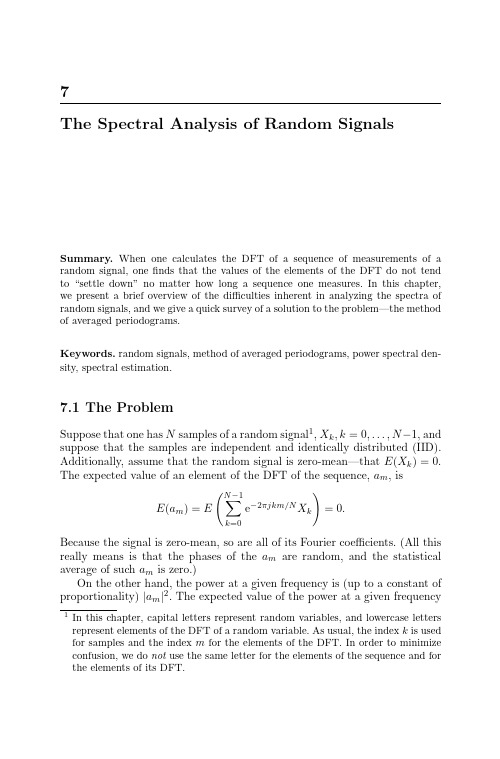
7The Spectral Analysis of Random Signals Summary.When one calculates the DFT of a sequence of measurements of a random signal,onefinds that the values of the elements of the DFT do not tend to“settle down”no matter how long a sequence one measures.In this chapter, we present a brief overview of the difficulties inherent in analyzing the spectra of random signals,and we give a quick survey of a solution to the problem—the method of averaged periodograms.Keywords.random signals,method of averaged periodograms,power spectral den-sity,spectral estimation.7.1The ProblemSuppose that one has N samples of a random signal1,X k,k=0,...,N−1,and suppose that the samples are independent and identically distributed(IID). Additionally,assume that the random signal is zero-mean—that E(X k)=0. The expected value of an element of the DFT of the sequence,a m,isE(a m)=EN−1k=0e−2πjkm/N X k=0.Because the signal is zero-mean,so are all of its Fourier coefficients.(All this really means is that the phases of the a m are random,and the statistical average of such a m is zero.)On the other hand,the power at a given frequency is(up to a constant of proportionality)|a m|2.The expected value of the power at a given frequency 1In this chapter,capital letters represent random variables,and lowercase letters represent elements of the DFT of a random variable.As usual,the index k is used for samples and the index m for the elements of the DFT.In order to minimize confusion,we do not use the same letter for the elements of the sequence and for the elements of its DFT.587The Spectral Analysis of Random Signalsis E(|a m|2)and is non-negative.If one measures the value of|a m|2for some set of measurements,one is measuring the value of a random variable whose expected value is equal to the item of interest.One would expect that the larger N was,the more certainly one would be able to say that the measured value of|a m|2is near the theoretical expected value.One would be mistaken.To see why,consider a0.We know thata0=X0+···+X N−1.Assuming that the X k are real,wefind that|a0|2=N−1n=0N−1k=0X n X k=N−1n=0X2k+N−1n=0N−1,k=nk=0X n X k.Because the X k are independent,zero-mean random variables,we know that if n=k,then E(X n X k)=0.Thus,we see that the expected value of|a0|2isE(|a0|2)=NE(X2k).(7.1) We would like to examine the variance of|a0|2.First,consider E(|a0|4). Wefind thatE(|a0|4)=NE(X4i)+3N(N−1)E2(X2i).(See Exercise5for a proof of this result.)Thus,the variance of the measure-ment isE(|a0|4)−E2(|a0|2)=NE(X4i)+2N2E2(X2i)−3NE2(X2i)=Nσ2X2+2(N2−N)E2(X2i).Clearly,the variance of|a0|2is O(N2),and the standard deviation of|a0|2is O(N).That is,the standard deviation is of the same order as the measure-ment.This shows that taking larger values of N—taking more measurements—does not do much to reduce the uncertainty in our measurement of|a0|2.In fact,this problem exists for all the a m,and it is also a problem when the measured values,X k,are not IID random variables.7.2The SolutionWe have seen that the standard deviation of our measurement is of the same order as the expected value of the measurement.Suppose that rather than taking one long measurement,one takes many smaller measurements.If the measurements are independent and one then averages the measurements,then the variance of the average will decrease with the number of measurements while the expected value will remain the same.Given a sequence of samples of a random signal,{X0,...,X N−1},define the periodograms,P m,associated with the sequence by7.3Warm-up Experiment59P m≡1NN−1k=0e−2πjkm/N X k2,m=0,...,N−1.The value of the periodogram is the square of the absolute value of the m th element of the DFT of the sequence divided by the number of elements in the sequence under consideration.The division by N removes the dependence that the size of the elements of the DFT would otherwise have on N—a dependence that is seen clearly in(7.1).The solution to the problem of the non-decreasing variance of the estimates is to average many estimates of the same variable.In our case,it is convenient to average measurements of P m,and this technique is known as the method of averaged periodograms.Consider the MATLAB r program of Figure7.1.In the program,MAT-LAB takes a set of212uncorrelated random numbers that are uniformly dis-tributed over(−1/2,1/2),and estimates the power spectral density of the “signal”by making use of the method of averaged periodograms.The output of the calculations is given in Figure7.2.Note that the more sets the data were split into,the less“noisy”the spectrum looks.Note too that the number of elements in the spectrum decreases as we break up our data into smaller sets.This happens because the number of points in the DFT decreases as the number of points in the individual datasets decreases.It is easy to see what value the measurements ought to be approaching.As the samples are uncorrelated,their spectrum ought to be uniform.From the fact that the MATLAB-generated measurements are uniformly distributed over(−1/2,1/2),it easy to see thatE(X2k)=1/2−1/2α2dα=α331/2−1/2=112=0.083.Considering(7.1)and the definition of the periodogram,it is clear that the value of the averages of the0th periodograms,P0,ought to be tending to1/12. Considering Figure7.2,we see that this is indeed what is happening—and the more sets the data are split into,the more clearly the value is visible.As the power should be uniformly distributed among the frequencies,all the averages should be tending to this value—and this too is seen in thefigure.7.3Warm-up ExperimentMATLAB has a command that calculates the average of many measurements of the square of the coefficients of the DFT.The command is called psd(for p ower s pectral d ensity).(See[7]for more information about the power spectral density.)The format of the psd command is psd(X,NFFT,Fs,WINDOW)(but note that in MATLAB7.4this command is considered obsolete).Here,X is the data whose PSD one would like tofind,NFFT is the number of points in each607The Spectral Analysis of Random Signals%A simple program for examining the PSD of a set of%uncorrelated numbers.N=2^12;%The next command generates N samples of an uncorrelated random %variable that is uniformly distributed on(0,1).x=rand([1N]);%The next command makes the‘‘random variable’’zero-mean.x=x-mean(x);%The next commands estimate the PSD by simply using the FFT.y0=fft(x);z0=abs(y0).^2/N;%The next commands break the data into two sets and averages the %periodograms.y11=fft(x(1:N/2));y12=fft(x(N/2+1:N));z1=((abs(y11).^2/(N/2))+(abs(y12).^2/(N/2)))/2;%The next commands break the data into four sets and averages the %periodograms.y21=fft(x(1:N/4));y22=fft(x(N/4+1:N/2));y23=fft(x(N/2+1:3*N/4));y24=fft(x(3*N/4+1:N));z2=(abs(y21).^2/(N/4))+(abs(y22).^2/(N/4));z2=z2+(abs(y23).^2/(N/4))+(abs(y24).^2/(N/4));z2=z2/4;%The next commands break the data into eight sets and averages the %periodograms.y31=fft(x(1:N/8));y32=fft(x(N/8+1:N/4));y33=fft(x(N/4+1:3*N/8));y34=fft(x(3*N/8+1:N/2));y35=fft(x(N/2+1:5*N/8));y36=fft(x(5*N/8+1:3*N/4));y37=fft(x(3*N/4+1:7*N/8));y38=fft(x(7*N/8+1:N));z3=(abs(y31).^2/(N/8))+(abs(y32).^2/(N/8));z3=z3+(abs(y33).^2/(N/8))+(abs(y34).^2/(N/8));z3=z3+(abs(y35).^2/(N/8))+(abs(y36).^2/(N/8));z3=z3+(abs(y37).^2/(N/8))+(abs(y38).^2/(N/8));z3=z3/8;Fig.7.1.The MATLAB program7.4The Experiment61%The next commands generate the program’s output.subplot(4,1,1)plot(z0)title(’One Set’)subplot(4,1,2)plot(z1)title(’Two Sets’)subplot(4,1,3)plot(z2)title(’Four Sets’)subplot(4,1,4)plot(z3)title(’Eight Sets’)print-deps avg_per.epsFig.7.1.The MATLAB program(continued)FFT,Fs is the sampling frequency(and is used to normalize the frequency axis of the plot that is drawn),and WINDOW is the type of window to use.If WINDOW is a number,then a Hanning window of that length is e the MATLAB help command for more details about the psd command.Use the MATLAB rand command to generate216random numbers.In order to remove the large DC component from the random numbers,subtract the average value of the numbers generated from each of the numbers gener-ated.Calculate the PSD of the sequence using various values of NFFT.What differences do you notice?What similarities are there?7.4The ExperimentNote that as two ADuC841boards are used in this experiment,it may be necessary to work in larger groups than usual.Write a program to upload samples from the ADuC841and calculate their PSD.You may make use of the MATLAB psd command and the program you wrote for the experiment in Chapter4.This takes care of half of the system.For the other half of the system,make use of the noise generator imple-mented in Chapter6.This generator will be your source of random noise and is most of the second half of the system.Connect the output of the signal generator to the input of the system that uploads values to MATLAB.Look at the PSD produced by MATLAB.Why does it have such a large DC component?Avoid the DC component by not plotting thefirst few frequencies of the PSD.Now what sort of graph do you get?Does this agree with what you expect to see from white noise?Finally,connect a simple RC low-passfilter from the DAC of the signal generator to ground,and connect thefilter’s output to the A/D of the board627The Spectral Analysis of Random SignalsFig.7.2.The output of the MATLAB program when examining several different estimates of the spectrumthat uploads data to MATLAB.Observe the PSD of the output of thefilter. Does it agree with what one expects?Please explain carefully.Note that you may need to upload more than512samples to MATLAB so as to be able to average more measurements and have less variability in the measured PSD.Estimate the PSD using32,64,and128elements per window. (That is,change the NFFT parameter of the pdf command.)What effect do these changes have on the PSD’s plot?7.5Exercises63 7.5Exercises1.What kind of noise does the MATLAB rand command produce?Howmight one go about producing true normally distributed noise?2.(This problem reviews material related to the PSD.)Suppose that onepasses white noise,N(t),whose PSD is S NN(f)=σ2N through afilter whose transfer function isH(f)=12πjfτ+1.Let the output of thefilter be denoted by Y(t).What is the PSD of the output,S Y Y(f)?What is the autocorrelation of the output,R Y Y(τ)? 3.(This problem reviews material related to the PSD.)Let H(f)be thefrequency response of a simple R-Lfilter in which the voltage input to thefilter,V in(t)=N(t),enters thefilter at one end of the resistor,the other end of the resistor is connected to an inductor,and the second side of the inductor is grounded.The output of thefilter,Y(t),is taken to be the voltage at the point at which the resistor and the inductor are joined.(See Figure7.3.)a)What is the frequency response of thefilter in terms of the resistor’sresistance,R,and the inductor’s inductance,L?b)What kind offilter is being implemented?c)What is the PSD of the output of thefilter,S Y Y(f),as a function ofthe PSD of the input to thefilter,S NN(f)?Fig.7.3.A simple R-Lfilter647The Spectral Analysis of Random Signalsing Simulink r ,simulate a system whose transfer function isH (s )=s s +s +10,000.Let the input to the system be band-limited white noise whose bandwidth is substantially larger than that of the fie a “To Workspace”block to send the output of the filter to e the PSD function to calcu-late the PSD of the output.Plot the PSD of the output against frequency.Show that the measured bandwidth of the output is in reasonable accord with what the theory predicts.(Remember that the PSD is proportional to the power at the given frequency,and not to the voltage.)5.Let the random variables X 0,...,X N −1be independent and zero-mean.Consider the product(X 0+···+X N −1)(X 0+···+X N −1)(X 0+···+X N −1)(X 0+···+X N −1).a)Show that the only terms in this product that are not zero-mean areof the form X 4k or X 2k X 2n ,n =k .b)Note that in expanding the product,each term of the form X 4k appears only once.c)Using combinatorial arguments,show that each term of the formX 2k X 2n appears 42times.d)Combine the above results to conclude that (as long as the samplesare real)E (|a 0|4)=NE (X 4k )+6N (N −1)2E 2(X 2k ).。


光谱线展宽的物理机制摘要本文首先介绍了原子光谱的形成和原子谱线的轮廓,以及用来定量描述谱线轮廓的三个物理量——谱线强度、中心频率和谱线半高宽。
接下来对光谱线展宽的各种物理机制作了定性或定量地分析。
详细地推导了谱线的自然展宽、多普勒展宽(高斯展宽)和洛伦兹展宽的半高宽公式。
并推导出了佛克脱半高宽、多普勒半高宽和洛伦兹半高宽之间的关系式。
给出了赫鲁兹马克展宽(共振展宽)的半高宽公式。
定性地分析了谱线的自吸展宽。
以类氢离子为例说明了同位素效应引起的同位素展宽。
定性地分析了原子的核自旋对谱线宽度的影响。
说明了在有外电场或内部不均匀强电场存在的情况下谱线会产生斯塔克变宽,在有外磁场存在的情况下谱线会产生塞曼变宽。
最后对光谱线展宽的各种物理机制做了一个简单的总结,指出光谱线展宽的实质是光的频率发生了变化,各种新频率光的叠加导致了光谱线的展宽。
并说明了对光谱线展宽的物理机制的研究,在提高光的单色性和物理量测量等方面具有重要的意义。
关键词:谱线展宽;物理机制;谱线轮廓;半高宽THE PHYSICAL MECHANISM OF SPECTRAL LINE BROADENINGABSTRACTFirstly, we introduce the formation of atomic spectrum and the outline of atomic spectral line in this paper, as well as three physical quantities—intensity of spectral line, center frequency and half width of spectral line profile which are used to describe spectral line profile quantitatively.Next we analyze various physical mechanism of spectral line broadening qualitatively or quantitatively. The natural half width of spectral line, half width of Doppler spectral line profile (Gaussian spectral line profile) and half width of Lorentz spectral line profile are derived detailedly. And the relationship of half width of Voigt spectral line profile, half width of Doppler spectral line profile and half width of Lorentz spectral line profile is also derived detailedly. We introduce Holtsmark broadening (resonance broadening) and give half width of Holtsmark spectral line profile. It is introduced qualitatively how the Self-absorption broadening affects spectral line profile. Taking Hydrogenic ions for an example, we explain isotope broadening caused by Isotope effect. Spectral line broadening caused by nuclear spin is analyzed qualitatively. Stark effect can cause Stark broadening when there is external electric field or internal non-uniform strong electric field, and Zeeman effect can cause Zeeman broadening when there is external magnetic field.Finally, we make a summary on the physilcal mechanism of spectral line broadening, pointing out spectral line broadening is essentially a change in the frequency of spectral lines, and superposition of various spectral lines having a new frequency component leads tospectral line broadening. The study on the physilcal mechanism of spectral line broadening has very important significance in many aspects, for example, the improving of spectral line's monochromaticity,the measurement of physical quantities and so on.KEY WORDS: spectral line broadening; physical mechanism; spectral Line profile; half width前言 (1)第一章原子谱线的轮廓 (2)§1.1 原子发光机理和光谱线的形成 (2)§1.2 原子谱线的轮廓 (2)第二章光谱线展宽的各种物理机制 (4)§2.1 自然宽度 (4)§2.2 多普勒展宽 (5)§2.3 洛伦兹展宽 (7)§2.4 赫鲁兹马克展宽 (9)§2.5 自吸展宽 (9)§2.6 佛克脱谱线宽度 (10)§2.7 谱线的超精细结构 (12)§2.7.1 同位素效应 (12)§2.7.2 原子的核自旋 (13)§2.8 场致变宽 (14)§2.8.1 斯塔克变宽 (14)§2.8.2 塞曼变宽 (15)总结 (17)参考文献 (18)致谢 (20)无论是原子的发射线轮廓或是吸收线轮廓,都是由各种展宽因素共同作用而成的。
Effects of culture conditions on ligninolytic enzymes and protease production by 1Phanerochaete chrysosporium in air23XU Zhenping1,2, WEN Xin1,*41. Research Center for Eco-Environmental Sciences, Chinese Academy of Sciences, Beijing 5100085, China. E-mail: jesc@62. Graduate School of Chinese Academy of Sciences, Beijing 100039, China78Abstract:The production of ligninolytic enzymes and protease by Phanerochaete 9chrysosporium was investigated under different culture conditions. Different amounts of 10medium were employed in free and immobilized culture, together with two kinds of medium 11with different C/N ratios. Little lignin peroxidase (LiP) (< 2 U/L) was detected in free culture 12with nitrogen-limited medium (56/2.2 m mol/L), while manganese peroxidase (MnP) 13maximum activity was 231 and 240 U/L in 50 and 100 ml medium culture, respectively.14Medium type had the greatest impact on protease production. Large amount of protease was 15produced due to glucose limitation. Culture type and medium volume influence protease 16activity corporately by affecting oxygen supply. The results implied shallow immobilized 17culture was a possible way to gain high production of ligninolytic enzymes.18Key words:protease; culture conditions; ligninolytic enzymes; Phanerochaete 19chrysosporium2021Introduction22The white rot fungus Phanerochaete chrysosporium has been extensively studied 23because of its powerful ligninolytic enzymes. These enzymes, mainly including lignin 24peroxidase (LiP) and manganese peroxidase (MnP), are secreted during the secondar y 25metabolism triggered by carbon, nitrogen or sulfur limitation (Cabaleiro et al., 2006;26Cabaleiro and Couto, 2007). They have been demonstrated to play a crucial role in lignin2728--------------------------------2930* Corresponding author. E-mail: jesc@.degradation and showed great potential in paper industry. At the same time, more and more 31researches have revealed that the ligninolytic enzymes are nonspecific enzymes and can assist 32in the degradation of a wide variety of recalcitrant organic pollutants, such as polycyclic 33aromatic hydrocarbons (PAHs), pesticide and dyes, as has been reviewed by Cameron et al.34(2000). This raised the interest of study in ligninolytic enzymes production.35In the present report, the fermentation was carried out in batches under air atmosphere.36The effects of culture conditions, including culture type, medium species, and the 37relationship between protease and ligninolytic enzymes, were discussed.38391 Materials and methods401.1 Plant material and growth conditions41Arabidopsis thaliana ecotype Columbia-0 (Col-0) was used in all experiments. Seeds 42were surface-sterilized with 75% ethanol, rinsed with water, and incubated for 2 d at 4℃, 43then distributed in commercial mixture medium and covered with glass for 48 h to ensure 44high humidity for an even germination. After growing for 10 d, young plants were 45transplanted to 6 cm × 6 cm plastic pots (5 plants in each pot) and grown in a greenhouse 46under 800 µmol/(m2·s) photosynthetically active radiation (PAR, 400--700 nm), supplied by 47400 W dysprosium lamps (Osram Powerstar, Germany). Spctrum of this type of dysprosium 48was shown in our former paper.49Fully expanded leaves (4th--6th leaf) were used as plant materials. Detached leaves with 50abaxial surface up floating on distilled water in Petri dish, were exposed to UV-B radiation at51a distance of 20 cm from the lamps, and without any other illumination.52531.2 UV-B and white light irradiantion54UV-B radiation (also containing UV-A) was obtained from 6 UVB-313 lamps (Q-PANEL, 55USA) and filtered through 0.13 mm cellulose diacetate. All radiation below 280 nm was 56filtered out. Measurement of spectral irradiance was the same as our privious report (Li et al., 572002a). Irradiance of the UV-B region (280--315 nm) was 2.95 W/m2. White light, 150 W/m2 58in the interval 400 to 700 nm, used for photorepair experiments, was supplied by a 400-W 59lamp (Osram Powerstar, Germany) and filtered through a 10-cm depth of water in a 60transparent polystyrene container to remove excess infrared radiation. Radiation 61measurements were carried out with a model 754-6S spectroradiomete (Optronic 62Laboratories, USA). Spectral irradiances of UV-B and white light for photorepair 63experiments were shown in our previous report.64652 Results (or Results and discussion)662.1 Cultured with different volumes of N-limited medium67In the 250 ml Erlenmeyer flasks with 50 or 100 ml nitrogen-limited medium, hyphal 68pellets were formed since day 2. After the pellets grew up to about 5 mm in diameter, spurs 69began to appear and MnP activity emerged in the medium ever since.70Different volumes of medium in flasks led to different nutrition consumption rates (Fig.711). On one hand, ammonium nitrogen was totally consumed in 2 d when 50 ml medium was 72added, but it was depleted on day 3 in cultures with 100 ml medium. On the other hand, faster 73average glucose consumption rate was found in 50 ml medium cultures, which are 0.407 and 740.845 g/(L·d) during the primary metabolism phase (0--4 d) and secondary metabolism phase 75(5--9 d). In 100 ml medium culture, glucose consumption rates are 0.337 and 0.810 g/(L·d) 76during these two phases.7778Fig. 1 Glucose, ammonium nitrogen concentration and MnP, LiP, protease activity curves during the free7980culture with N-limited medium.812.2 Immobilized cultures82Since the immersion status of the support in the medium had effect on ligninolytic 83enzymes production (Couto et al., 1998, 2000), in 50 and 100 ml nitrogen limited medium, 840.9 and 1.8 g polyurethane foam carriers was added, respectively. This made both of these 85two culture systems in critical immersed conditions. Raw water characters are shown in Table 861.8788899091Table 1 Qualities of raw domestic wastewaterParameter Range MeanpH 7--8 7.5COD (mg/L) 200--600 400NH4+-N (mg/L) 30--50 40TN (mg/L) 40--60 50TP (mg/L) 7--12 992Fewer mediums in the flask promoted ammonium nitrogen and glucose consumption by 93fungus. In 50 ml-medium system ammonium nitrogen was depleted on day 1 while it cost 2 d 94for complete nitrogen consumption in 100 ml-medium system. Glucose disappeared at a rate 95of 1.372 g/(L·d) during the whole fermentation process in 50 ml medium flask, which is 96faster than the rate of 0.911 g/(L·d) in 100 ml medium flask (Fig. 2). Comparing results got in 97free and immobilized cultures, we can see that immobilization greatly improved nutrition 98take-in speed.99100101Fig. 2 Glucose, ammonium nitrogen concentration and MnP, LiP, protease activity curves during the 102immobilized culture with N-limited medium.1033 Discussion1043.1 Ligninolytic enzymes production105To promote ligninolytic enzymes production in large scale, harvesting these products 106during fermentation in air is undoubtedly of great significance. MnP formation was generally 107less affected by oxygen level (Rothschild et al., 1999) and its production can be easily 108achieved in flasks or reactors with commonly used nitrogen-limited medium when exposed to 109air (Couto et al., 2001). This viewpoint is also demonstrated in the present research because 110high MnP activity in all cultures with nitrogen-limited medium.1111123.2 Protease production113Since protease is a factor, which may influence ligninolytic enzymes stability during the 114culture of P. chrysosporium, studying the effect of culture conditions on protease production 115is helpful to direct fermentation process aiming at stable enzymes production.1163 Conclusions117This study clearly demonstrated that anti-androgenic p,p'-DDE could induce intersex 118testis in Japanese medaka at 100 μg/L level after two-month exposure. VTG-1 and VTG-2 119were both found to be significantly up-regulated by p,p'-DDE with dose-dependant 120relationships, suggesting that they can also be used as biomarkers for anti-androgenic 121p,p'-DDE.122123Acknowledgments124125This work was supported by the National Natural Science Foundation of China (No. XXXXXX) and the National Basic Research Program (973) of China (No. XXXXXX). We are grateful to Prof. Sieve 126127Huang for his valuable advice regarding statistical analysed.128References129APHA (American Public Health Association), AWWA (American Water Works Association), 130and WEF (Water Environment Federation), 1999. Standard methods for the examination 131of water and wastewater (20th ed.). Washington DC, USA.132Bingner R L, Theurer F D, 2001. AnnAGNPS: estimating sediment yield by particle size for 133sheet and rill erosion. In: Proceedings of the Seventh Interagency Sedimentation 134Conference, the Sediment: Monitoring, Modeling and Managing. Reno, NV. 25--29 135March. Vol. I: 1--7.136Cabaleiro D R, Couto S R, 2007. Comparison between the protease production ability of 137ligninolytic fungi cultivated in solid-state media. Journal of Environmental Sciences, 13819(9): 1017--1023.139Cabaleiro D R, Rodriguez S, Sanroman A, Willsion W, 2006. Characterisation of 140deactivating agents and their influence on manganese-dependent peroxidase from 141Phanerochaete chrysosporium. Journal of Environmental Sciences, 18(7): 867--872.142Cameron M D, Timofeevski S, Aust S D, 2000. Enzymology of Phanerochaete 143chrysosporium with respect to the degradation of recalcitrant compounds and 144xenobiotics.Applied Microbiology and Biotechnology, 54(6): 751--758.145Couto S R, 1998. Effect of veratryl alcohol and manganese (IV) oxide on ligninolytic activity 146in semi solid cultures of Phanerochaete chrysosporium. Biodegradation, 9(2): 143--150. 147Couto S R, 2000. Stimulation of ligninolytic enzyme production and the ability to decolourise 148Poly R-478 in semi-solid-state cultures of Phanerochaete chrysosporium. 149Environmental Science Technology, 74(2): 159--164.150Dosoretz C G, Chen H C, Grethlein H E, 2007. Effect of environmental conditions on 151extracellular protease activity in ligninolytic cultures of Phanerochaete chrysosporium. 152Journal of Environmental Sciences, 19(12): 1395--1400.153Dosoretz C, Chen H C, Grethlein H E, 2007a. Effect of oxygenation conditions on submerged 154cultures of Phanerochaete chrysosporium. Journal of Environmental Sciences,19(2): 155131--137.156Gomez K A, Gomez A A, 1984. Statistical Procedures for Agricultural Research. 157International Rice Research Institute, New York, USA. 680.158Lee M T, White D C, 1992. Application of GIS databases and water quality modeling for 159agricultural non-point source pollution control. In: Research Report No. 014 of Water 160Resources Center, University of Illinois at Urbana-Champaigne. Urbana, IL, USA.161Rihn M J, Zhu X, Suidan M T, Kim B J, Kim B R, 1997. The effect of nitrate on VOC 162removal in trickle bed biofilters. Water Research, 31(12): 2997--3008.163Tipping E, 2002. Cation binding by humic substances. In: Rapid Detection Assays for Food 164and Water (Thompson K C, Keevil C E, eds). New York: Cambridge University Press. 165175--177.166167168169List of figure captionsFig. 1 Concentrations of Si-HCl (a), Si-Alk (b) and t-BSi (c) in August and February intertidal sediments 170171of the Yangtze Estuary. Error bars represent the standard deviation of replicate (n = 3) sediment samples. 172Fig. 2 Plasma vitellogenin levels in juvenile male goldfish of controls (blank, solvent and postive)andthose exposed to 1,2,3,7,8-PeCDD at the doses of 1/4LD 50 (0.46 mg/kg), 1/2LD 50 (0.92 mg/kg), and LD 30 173 (1.63 mg/kg) for seven days and fourteen days separately. Values were means ± S.D. * P < 0.01.174Si-Alk (µmol Si/g)t-BSi (µmol Si/g)Si-HCl (µmol Si/g)175 Fig. 1 Concentrations of Si-HCl (a), Si-Alk (b) and t-BSi (c) in August and February intertidal sediments176 of the Yangtze Estuary. Error bars represent the standard deviation of replicate (n = 3) sediment 177 samples.178179100020003000400050006000500006000070000V i t e l l o g e n i n C o n c e n t r a t i o n (n g /m L )Dose180 Fig. 2 Plasma vitellogenin levels in juvenile male goldfish of controls (blank, solvent and postive) and those 181 exposed to 1,2,3,7,8-PeCDD at the doses of 1/4 LD 50 (0.46 mg/kg), 1/2LD 50 (0.92 mg/kg), and LD 30 (1.63 182 mg/kg) for seven days and fourteen days separately. Values were means ± S.D. * P < 0.01.183184。
第45卷 第1期2021年1月激 光 技 术LASERTECHNOLOGYVol.45,No.1January,2021 文章编号:1001 3806(2021)01 0121 05光电成像系统的绝对光谱响应效率测量及分析陈均溢,商思航,苗 丹,江财俊,曾延安(华中科技大学光学与电子信息学院光电工程系,武汉430074)摘要:为了准确测量光电成像系统的绝对光谱响应效率,采用光学系统光能量传递公式以及图像传感器的物理模型,得到了光电成像系统绝对光谱响应效率的计算公式,在此基础上设计了基于积分球、多光谱发光二极管光源、标准探测器及透射式平行光管的光电成像系统绝对光谱响应效率测量装置,并对光谱响应效率已知的可见光数字相机进行实验测量和分析。
结果表明,在380nm~1100nm波长范围内测量装置测得的可见光数字相机的绝对光谱响应效率与标准值具有较好的一致性,最大相对误差为1.7%,各波长点的测量不确定度在置信概率为95%时均小于0.2%,满足一般的测量要求。
该装置能够准确地对光电成像系统的绝对光谱效应效率进行测量。
关键词:成像系统;图像传感器;绝对光谱响应;标准探测器中图分类号:TN247 文献标志码:A doi:10 7510/jgjs issn 1001 3806 2021 01 021MeasurementandanalysisofabsolutespectralresponseefficiencyofphotoelectricimagingsystemCHENJunyi,SHANGSihang,MIAODan,JIANGCaijun,ZENGYan’an(DepartmentofOptoelectronicEngineering,SchoolofOpticalandElectronicInformation,HuazhongUniversityofScienceandTechnology,Wuhan430074,China)Abstract:Inordertoaccuratelymeasuretheabsolutespectralresponseefficiencyofthephotoelectricimagingsystem,theopticalenergytransferformulaoftheopticalsystemandthephysicalmodeloftheimagesensorwereanalyzed,andthecalculationformulaoftheabsolutespectralresponseefficiencyofthephotoelectricimagingsystemwasobtained.Basedonthetheoreticalformula,anabsolutespectralresponseefficiencymeasurementdeviceforthephotoelectricimagingsystembasedonintegratingspheres,multispectrallightsourceoflight emittingdiode,standarddetector,andatransmission typeparallellighttubewasdesigned.Experimentalmeasurementandanalysisofvisiblelightdigitalcameraswithknownspectralresponseefficiencywascarriedout.Theresultsshowthat,theabsolutespectralresponseefficiencyofthevisiblelightdigitalcamerameasuredbythemeasuringdeviceinthewavelengthrangeof380nm~1100nmisingoodagreementwiththestandardvalue,andthemaximumrelativeerroris1.7%.Whentheprobabilityis95%,itislessthan0.2%,whichmeetsthegeneralmeasurementrequirements.Thedevicecanaccuratelymeasuretheabsolutespectraleffectefficiencyofthephotoelectricimagingsystem.Keywords:imagingsystems;imagesensor;absolutespectralresponse;standarddetector 作者简介:陈均溢(1995 ),男,硕士研究生,现主要从事光电探测及光电成像相关领域的研究。
拉曼光谱测量钙钛矿电声耦合强度1.拉曼光谱是一种用于分析晶体材料结构和性质的强大技术。
Raman spectroscopy is a powerful technique for analyzing the structure and properties of crystalline materials.2.钙钛矿是一类具有重要电声耦合特性的材料。
Perovskite is a type of material with important electroacoustic coupling properties.3.通过拉曼光谱,可以了解钙钛矿中电声耦合的强度和机制。
Raman spectroscopy can be used to understand the strength and mechanism of electroacoustic coupling in perovskite.4.钙钛矿的电声耦合特性对于光伏和光电器件的性能至关重要。
The electroacoustic coupling properties of perovskite are crucial for the performance of photovoltaic and optoelectronic devices.5.拉曼光谱可以提供关于晶体结构、相变和电子结构的丰富信息。
Raman spectroscopy can provide rich information about crystal structure, phase transitions, and electronic structure.6.钙钛矿材料的电声耦合性质直接影响着其光电器件的效率和稳定性。
The electroacoustic coupling properties of perovskite materials directly affect the efficiency and stability oftheir optoelectronic devices.7.拉曼光谱测量可以帮助科学家们深入了解钙钛矿材料的微观特性。
a r X i v :a s t r o -p h /0502387v 1 19 F eb 2005Draft version February 5,2008Preprint typeset using L A T E X style emulateapj v.6/22/04MEASUREMENT OF SPECTRAL BREAKS IN PULSAR WIND NEBULAE WITH MILLIMETER-WAVEINTERFEROMETRYD.C.-J.Bock 1Radio Astronomy Laboratory,University of California,Berkeley,CA 94720andB.M.GaenslerHarvard-Smithsonian Center for Astrophysics,60Garden Street MS-6,Cambridge,MA 02138Draft version February 5,2008ABSTRACTWe have observed pulsar wind nebulae in the three supernova remnants G11.2−0.3,G16.7+0.1,and G29.7−0.3at 89GHz with the Berkeley-Illinois-Maryland Association Array,measuring total flux densities of two of them for comparison with archival data at other frequencies.In G16.7+0.1,we find a break in the spectrum of the PWN at ∼26GHz.In G29.7−0.3,our data suggest a break in the integrated spectrum of the central nebula at ∼55GHz,lower than previously estimated.However,we have found spatial structure in the spectrum of this nebula.The emission to the north of pulsar J1846−0258has a broken spectrum,with break frequency 100GHz,consistent with a conventional pulsar-powered nebula.The emission to the south of the pulsar has a near-power-law spectrum from radio to X-rays:this component may be unrelated to the PWN,or may be evidence of asymmetries and/or time evolution in the pulsar’s energy output.We present 89GHz images of each remnant.Subject headings:pulsars:individual (J1846−0258)—radio continuum:ISM—SNR:individual(G11.2−0.3,G16.7+0.1,G29.7−0.3)—supernova remnants1.INTRODUCTIONPulsars are born spinning with up to 1051erg of ro-tational kinetic energy —as much energy as in the su-pernovae in which they are born.This vast reservoir of energy is ultimately deposited into the ambient medium through the pulsar’s relativistic wind.In many cases,this interaction between the pulsar and its environment is directly observable,in the form of a synchrotron-emitting pulsar wind nebula (PWN),of which the Crab Nebula is the best-known example.While many pulsars have their beams directed away from us,PWNe radiate isotropi-cally.Thus PWNe are powerful probes of pulsars and their energy loss,even when the pulsar itself cannot be detected.At radio frequencies,PWNe typically have flat spec-tra −0.3<α<0(S ν∝να),but in the X-ray band we generally see α<−1.It is therefore com-monly presumed that PWNe have at least one spec-tral break at intermediate wavelengths.Such breaks are expected from theoretical considerations,and re-sult from a combination of synchrotron losses and the time-evolution of the pulsar’s changing energy out-put (Pacini &Salvati 1973;Reynolds &Chevalier 1984;Woltjer et al.1997).Locating these breaks gives insight into the physical conditions of the pulsar wind:in PWNe powered by young (<5kyr)pulsars,the spectral break can be used to infer directly the nebular magnetic field strength (e.g.Manchester,Staveley-Smith,&Kesteven 1993),while spatial variations in the break energy can be used to identify and map out the processes of particle dif-fusion and radiative losses within the flow (Amato et al.2000;Bock,Wright,&Dickel 2001).Electronic address:dbock@ Electronic address:bgaensler@1present address:CARMA,P.O Box 968,Big Pine,CA 93513Most flux density measurements of PWNe to date have been in the X-ray and low-frequency radio bands.To pin down the break frequencies it is necessary to measure flux densities in the part of the spectrum near the spectral breaks,i.e.at millimeter and infrared wavelengths.Here we report on observations of three PWNe for which extant data at radio and X-ray wavelengths implied a spectral break in or below the mm band.The PWNe,in the supernova remnants G11.2−0.3,G16.7+0.1,and G29.7−0.3(Kesteven 75),were iden-tified from the catalog of Green (2004)as being suffi-ciently bright and compact to allow imaging with mil-limeter interferometers.Two of the PWNe (in G11.2−0.3and G29.7−0.3)contain young X-ray pulsars (Torii et al.1997;Gotthelf et al.2000).Only a few PWNe have been reliably imaged at millimeter wavelengths with sin-gle dish telescopes,and prior to this study only one (G21.5−0.9;Bock et al.2001)had been imaged with a millimeter interferometer.We have been able reliably to image two of the sources observed (in the supernova remnants G16.7+0.1and G29.7−0.3),obtaining their total flux densities at 89GHz.This has allowed us to determine the frequency of their spectral breaks at radio wavelengths using archival data and assuming the presence of a solitary break.We have been able to resolve the PWN in G29.7−0.3,letting us compare the millimeter-wave structure of the PWN with that in the X-ray band and at lower radio frequen-cies.We also present a millimeter-wave image of the SNR G11.2−0.3,which has a PWN with radio spectral indexα=−0.25+0.05−0.10(Tam,Roberts,&Kaspi 2002).How-ever,its extension compared to the spatial sensitivity of the array precludes any quantitative analysis.2Bock &Gaensler2.OBSERVATIONSObservations were obtained at 88.6GHz using the BIMA Array 2(Welch et al.1996)during 2002and 2003(Table 1).To achieve suitable uv coverage,we used the technique of multi-frequency synthesis over both 800MHz sidebands of the local oscillator.We measured only the left circular polarization (in the sense of IEEE 1969)in the assumption that circularly polarized emission from the sources would be negligible.3In order to image fully the extended structure,and to assist with the recovery of low spatial frequency information,we imaged each source with a 7-point hexagonal mosaic.The primary beam of the 6.1-m antennas is Gaussian with FWHM 2.′13.The short interferometer spacings (as low as 6.1m when antennas are nearly shadowed)available from the array provide significant sensitivity on spatial scales up to an arcminute.The shortest physical baselines are 8.1m.The bright quasars QSO B1730−130(for G11.2−0.3and G16.7+0.1)and QSO B1741-038(for G29.7−0.3)were observed as phase calibrators at 25to 30minute intervals,after 3complete cycles of 7pointings.We ex-pect the astrometric accuracy of the images to be bet-ter than 1arcsec,a precision routinely obtained with the BIMA Array (Looney &Hardcastle 2000).Single sideband system temperatures during the observations were between 200and 600K (scaled to outside the atmosphere).We used the on-line absolute flux den-sity scale determined from many observations of plan-ets,which have been found on average to be stable over time (Muhleman &Berge 1991).As a check we observed Uranus for 10minutes during each observing session,finding a day-to-day scatter for the mean gain on all an-tennas between 0.95and 1.12,implying multiplicative corrections to the flux density scale of between 0.91and 1.25.The mean correction would be 1.09for observa-tions of G16.7+0.1and 1.05for G29.7−0.3.The gains for each sideband were consistent within a few percent on each day.In this paper we retain the on-line scale,and note that with several days’observations contribut-ing to each image our measurements are consistent with an uncertainty in the overall flux density scale of about 10%.Imaging was done with the MIRIAD software pack-age (Sault,Teuben,&Wright 1995),using SDI decon-volution (Steer,Dewdney,&Itoh 1984):such CLEAN-based algorithms are generally superior to maximum en-tropy methods for low signal to noise ratios (Helfer et al.2003).The multiple pointing centers were combined into a mosaiced image corrected for the primary beam.To assess the reliability of flux density recovery when imag-ing these sources,simulations of each observation were made with MIRIAD,using the actual observations as a template.The results of the simulations are presented with the data on each source in the next section.3.RESULTS2The BIMA Array was operated until June 2004by the Berkeley-Illinois-Maryland Association with support from the Na-tional Science Foundation.3The BIMA Array natively measured one linear polarization.To convert to circular polarization,90-GHz quarter-wave plates were used.Fig.1.—Image of G11.2−0.3at 89GHz (contours)and 8.6GHz (grayscale;Roberts et al.2003).The contours are at 10,20,and 30mJy beam −1.The synthesized beam at 89GHz is shown at the lower right.3.1.G11.2−0.3The BIMA image of G11.2−0.3is shown with con-tours in Figure 1,overlaid upon an 8.6GHz image of Roberts et al.(2003).Based on positional coincidence with the 8.6GHz emission,we appear to have detected the PWN in this remnant (the single contour at the cen-ter of the image).However,the extended structure in the PWN is not well imaged by the array:the model-ing described in section 2showed that we have measured only approximately 10%of the emission,indicating that the PWN is nearly resolved out on all baselines.Given the magnitude and unreliability of the correction factor required to estimate the true flux density,we do not be-lieve that these data can provide a reliable estimate of the flux density of the PWN.High sensitivity single dish measurements would be required to investigate this ob-ject further.3.2.G16.7+0.1The PWN in this remnant (Figure 2)is detected as a peak of 14mJy beam −1at 8h 20m 57.s 2−14◦19′34′′(J2000).The feature is extended:an elliptical Gaussian fitted to the feature has a size of 51′′×20′′(at position angle 6◦east of north),and an integrated flux density of 27mJy.The size and position are consistent with the measurements of Helfand et al.(1989).To assess the reliability of this measurement we have modeled the response of the array to two simple sources:a 25′′×7′′Gaussian with major axis 10◦west of north and a 45′′×15′′Gaussian with major axis 20◦west of north,corresponding approximately to the 50%and 20%contours in the 2cm image of Helfand et al.(1989).In deconvolved images we recovered 97%and 80%of the total emission respectively,without taking into account a small residual negative background.We conclude that we should have measured at least 90%of the emission from this object,and consider that we have reliably de-termined the flux density of the PWN at this frequency.Spectral Breaks in Pulsar Wind Nebulae3 TABLE1Summary of observationsTime on Synthesized Beamof intersection of the Helfand et al.radio spectrum and a simple radio/X-ray spectrum (i.e.assuming a single break between X-ray and radio wavelength)consistent with the 89GHz and X-ray uncertainties.This pro-vides one way to quantify the uncertainty in the break frequency:the region has minimum and maximum fre-quencies (shown by the outer dotted lines)of 16and 42GHz respectively,leading to an estimate of the break frequency of 26+16−10GHz.The PWN in G16.7+0.1has one of the lowest known break frequencies in a PWN:breaks at lower or compa-rable frequencies have been reported only in G27.8+0.64We chose this image for a model owing to its higher signal to noise.Recalling the flat PWN spectrum in the radio,we do not believe that the difference between the PWN shape at the two frequencies will significantly affect our result.X-ray spectrum.Presumably this is not the result of inverse Compton scattering,which is generally expected to be significant at γ-ray wavelengths.This phenomenon has been seen in one other PWN,that around the pulsar PSR B1757−24(Kaspi et al.2001).5In that case,the X-ray and radio spectra are also approximately flat,with a steeper spectrum required to connect the radio and X-ray observations.However,whereas Kaspi et al.found that the X-ray spectrum was just marginally consistent with the implied radio to X-ray average spectrum,this possi-bility is very unlikely in the case of G16.7+0.1,where the average radio to X-ray spectrum is not consistent with5A step like that in the spectrum of the Crab Nebula at in-frared/optical wavelengths,thought due to dust reradiation or ex-tinction (Manchester &Taylor 1977),would not show up in the bulk radio to X-ray spectral index in the same way.Spectral Breaks in Pulsar Wind Nebulae5the X-ray data even within the90%uncertainty limits of Helfand et al.(2003a).One explanation for spectra of this shape is given by Reynolds&Chevalier(1984).They calculate that a combination of older particles suffering synchrotron losses due to compression of the magneticfield by the reverse shock and particles injected after the shock can give rise to a spectrum of this shape.However,whereas the reserve shock is expected to arrive after about104 years,Helfand et al.(2003a)have estimated G16.7+0.1 to be only about2000years old.Therefore this seems like an unlikely explanation for this source.4.2.G29.7−0.3:Integrated Spectrum of the PWN An integrated spectrum of the central nebula in G29.7−0.3is plotted in Figure4.This object wasfirst seen by Becker&Kundu(1976),who measured a radio spectral index of−0.27,flatter than that of the SNR shell.VLA observations(Becker&Helfand1984)con-firmed the discovery but implied aflat(α=0.0)spec-trum.Hunt et al.(as reported by Salter et al.1989)from different VLA observations obtained integratedflux den-sity measurements that imply a radio spectral index of −0.30.Both sets of VLA observations are plotted in Fig-ure4.We have measured aflux density of343mJy for the PWN in the recent1.4GHz data of Helfand et al. (2003b),consistent with the Salter et al.result.At higher frequencies,Morsi&Reich(1987b)mea-sured0.28Jy from the PWN at30GHz,but note that they could have suffered from confusion(their observa-tions had resolution26.′′5),leading to an overestimated result.It seems possible that they measured some of the broad underlying shell-related emission as well,which was not imaged at89GHz,and could have been poorly imaged at lower radio frequencies.This could have led to a further overestimate.As noted earlier(§3.3)we con-sider the Salter et al.84GHz measurement also to be an overestimate,for similar reasons.Combined with the Salter et al.lower-frequency mea-surements,the X-ray data of Helfand et al.(2003b),and assuming a simple unbroken spectrum between radio and X-ray wavelengths,our observations imply a spectral break at approximately55GHz(shown by the right-hand vertical dotted line in thefigure).Assuming the break to be sharp,the integratedflux density of the PWN at this frequency would be about120mJy beam−1.Allow-ing the spectrum above and below the putative break to vary within the uncertainties of the measurements im-plies that the break should fall within the shaded gray area,with a minimum frequency of21GHz(left-hand vertical line).The break is not strictly constrained at high frequencies,since a straight line is just consistent with the low-frequency Hunt et al.measurements and our89GHz measurement.However,it is likely that the break is below89GHz.We could alternatively have used the centimeter-wave data of Becker&Helfand(1984)and obtained a some-what lower break frequency.However,given the agree-ment between the data of Salter et al.and Helfand et al. (2003b),and the fact that the Salter et al.data were quoted with uncertainties,we prefer the later measure-ments.4.3.G29.7−0.3:Lobes of the PWN?The high resolution X-ray data clearly show two lobes of emission,to the north and south of the pulsar.The northern lobe is brighter at X-ray wavelengths.A com-parison of images of the PWN at1.4GHz,89GHz and in X-rays(Figure5)reveals that the PWN spectrum is also asymmetric.At1.4GHz,the PWN is brighter south of the pulsar,while at89GHz and above it is brighter north of the pulsar.These two components may have different origins,causing an integrated spectrum to be difficult to interpret.In Table2,we showflux densities of these northern and southern lobes,integrated over the regions shown in Figure5.The regions chosen were a compromise between the competing desires to minimize contamina-tion from the background and to include the majority of emission at each frequency.The area around the pul-sar was excluded from all datasets,avoiding the need to estimate an X-ray background for normalizing the inte-grated areas.At89GHz the same background as in§2 was subtracted.Helfand et al.(2003b)were not able to find a significant difference between the X-ray spectra of the northern and southern lobes,so the X-rayflux den-sities quoted correspond to the luminosity reported by Helfand et al.,apportioned according to the total counts in the two regions,assuming a uniform X-ray spectrum across the PWN.The89GHz uncertainties quoted are as in section2,those for X-rays are the standard errors for a Poisson distribution,and we assign an uncertainty of 10%to the1.4GHz measurements,to account for imag-ing errors.This is probably an overestimate of the true uncertainty at1.4GHz.Given the differing resolutions and systematic errors of the three datasets6,the results are necessarily quali-tative.However,as may be seen in Figure6,the north-ern lobe not only has aflatter spectrum on average,but shows strong evidence for break.Meanwhile,the spec-trum of the southern lobe may be unbroken.In thefig-ure,the uncertainties at radio frequencies are of order the point size,while those of the X-ray values are much smaller.The excellent positional agreement of the SNR shell at1.4and89GHz confirms the registration of the images.We believe that the difference in spectral shape between the lobes is reliable.The same result may be obtained qualitatively by con-volving the1.4GHz and X-ray observations to the reso-lution of the89GHz data(Figure7).For this analysis, a background estimated at24counts/pixel was substi-tuted for X-ray emission from the pulsar before convolu-tion.From thefigure,it is clear that the trend of steeper emission to the south holds.Although the systematic uncertainties are different,this method again implies a break in the spectrum of the northern lobe,and allows the southern lobe to have a simple power law spectrum from radio to X-rays.The simplest explanation for the difference in spec-trum to the north and south of the pulsar is that we are seeing both PWN and shell emission superimposed.In this scenario,a majority of the steep-spectrum emission seen at1.4GHz is attributed to the shell,seen near the pulsar due to projection.Other1.4-GHz emission pre-sumably from the shell may be seen at to the east of the 6In the89GHz image,there are only3beam areas within the northern region.6Bock &GaenslerFig.5.—Images of G29.7−0.3at (left to right)1.4GHz (Helfand et al.2003b),89GHz,and 0.5–10keV (Chandra archive;as presented by Helfand et al.2003b),showing the regions over which emission was integrated in the southern and northern lobes.TABLE 2Flux densities of the lobes around the pulsar in G29.7−0.3Flux Density (uncertainty)Frequency(mJy)Spectral Breaks in Pulsar Wind Nebulae7 Fig.7.—As for Figure5,all convolved to the resolution of the89GHz image.The position of PSR J1846−0258has been marked witha cross.for G16.7+0.1we expect afield of∼2.5mG,while forG29.7−0.3we expect>1.5mG.These values are sub-stantially higher than inferred in other remnants fromequipartition arguments,or more directly in the CrabNebula(e.g.Hester et al.1996),and seem to indicatethat standard synchrotron losses alone are not the originof the breaks.We are left with the conclusion that perhaps these areindeed remnants of a“second kind”(Woltjer et al.1997),in which intrinsic processes result in a spectrum differ-ent from that of the Crab.One possibility is that thepulsar’s excitation has decreased substantially at somepoint(Green&Scheuer1992),with the break moving tolower frequencies with time(Woltjer et al.1997).Alter-natively the pulsar injection spectra may not be a simplepower law.5.CONCLUSIONSWe have carried out observations of three pulsar windnebulae at millimeter wavelengths with the Berkeley-Illinois-Maryland Association Array.One of thesePWNe,in the SNR G11.2−0.3,was not adequately im-aged to allow quantitative analysis.Wefind the breakfrequency of the PWN in G16.7+0.1to be at about26GHz,and see an unusual upturn in the spectrum be-low or in the X-ray band.In only one other PWN,thatsurrounding PSR B1757−24,has a similar effect beenimplied.The bulk spectrum of the PWN in G29.7−0.3indicatesa likely spectral break at55GHz,but our observationsand previous data reveal a marked variation in spectrumacross the PWN.The spectrum is steeper to the southof the pulsar.It may be that the southern emission doesnot represent the continuing effect of the pulsar,but cor-responds to a part of the SNR shell seen in projection.However,we cannot account for the one-sided PWN un-der this scenario.The number of PWNe for which an analysis likethis may be made is limited by the large size of thePWNe compared to the spatial scales on which mil-limeter interferometers are sensitive.However,the sen-sitivity and resolution of next generation instruments,such as ALMA,will allow these investigations to beconducted on much larger samples in other galaxies.Meanwhile,improved single-dish mapping techniquesand sensitive wide-field imaging interferometers suchas CARMA could enhance the high-frequency data onGalactic PWNe.We thank E.Gotthelf,D.Helfand,and M.Robertsfor making available their data in electronic form,andM.Wright for useful discussions.This work has made useof the NASA ADS and was partially supported by NSFgrants AST-9981308and AST-0228963to the Universityof California,Berkeley.REFERENCESAmato,E.,Salvati,M.,Bandiera,R.,Pacini,F.,&Woltjer,L.2000,A&A,359,1107Becker,R.H.&Helfand,D.J.1984,ApJ,283,154Becker,R.H.&Kundu,M.R.1976,ApJ,204,427Bock,D.C.-J.,Wright,M.C.H.,&Dickel,J.R.2001,ApJ,561,L203Blondin,J.M.,Chevalier,R.A.,&Frierson,D.M.2001,ApJ,563,806Camilo,F.,et al.2002,ApJ,571,L41Gaensler,B.M.,van der Swaluw,E.,Camilo,F.,Kaspi,V.M.,Baganoff,F.K.,Yusef-Zadeh,F.,&Manchester,R.N.2004,ApJ,616,383Green D.A.,2004,Bulletin of the Astronomical Society of India,32,335Green,D.,&Scheuer,P.1992,MNRAS,258,943Gotthelf,E.V.,Vasisht,G.,Boylan-Kolchin,M.,&Torii,K.2000,ApJ,542,L37Helfand,D.J.,Ag¨u eros,M.A.,&Gotthelf,E.V.2003a,ApJ,592,941Helfand,D.J.,Collins,B.F.,&Gotthelf,E.V.,2003b,ApJ,582,783Helfand,D.J.,Velusamy,T.,Becker,R.H.,&Lockman,F.J.1989,ApJ,341,151Helfer,T.T.,Thornley,M.D.,Regan,M.W.,Wong,T.,Sheth,K.,Vogel,S.N.,Blitz,L.,&Bock,D.C.-J.2003,ApJS,145,259Hester,J.J.et al.1996,ApJ,456,225IEEE,1969,Standard Definitions of Terms for Radio WavePropagation,IEEE Trans.AP-17,270-275Kaspi,V.M.,Gotthelf,E.V.,Gaensler,B.M.,&Lyutikov,M.2001,ApJ,562,L163Looney,L.W.&Hardcastle,M.J.2000,ApJ,534,172Manchester,R.N.,Staveley-Smith,L.,&Kesteven,M.J.1993,ApJ,411,756Manchester,R.N.,&Taylor,J.H.1977,Pulsars(San Francisco:W.H.Freeman)Mereghetti,S.,Bandiera,R.,Bocchino,F.,&Israel,G.L.2002,ApJ,574,873Morsi,H.W.&Reich,W.1987a,A&AS,69,533Morsi,H.W.&Reich,W.1987b,A&AS,71,1898Bock&GaenslerMuhleman,D.O.&Berge,G.L.1991,Icarus,92,263Pacini,F.&Salvati,M.1973,ApJ,186,249Reich,W.,F¨u rst,E.,&Sofue,Y.1984,A&A,133,L4 Reynolds,S.P.&Chanan,G.A.1984,ApJ,281,673 Reynolds,S.P.&Chevalier,R.A.1984,ApJ,278,630 Roberts,M.S.E.,Tam,C.R.,Kaspi,V.M.,Lyutikov,M.,Vasisht, G.,Pivovaroff,M.,Gotthelf,E.V.,&Kawai,N.,2003,ApJ,588, 992Salter,C.J.,Reynolds,S.P.,Hogg,D.E.,Payne,J.M.,&Rhodes, P.J.1989,ApJ,338,171Sault,R.J.,Teuben,P.J.,&Wright,M.C.H.1995,in ASP Conf. Ser.77,Astronomical Data Analysis Software and Systems IV, ed.R.A.Shaw,H.E.Payne,&J.J.E.Hayes(San Francisco: ASP),433Steer,D.G.,Dewdney,P.E.,&Ito,M.R.1984,A&A,137,159 Tam,C.,Roberts,M.S.E.,&Kaspi,V.M.2002,ApJ,572,202 Torii,K.,Tsunemi,H.,Dotani,T.,&Mitsuda,K.1997,ApJ,489, L145Welch,W.J.et al.1996,PASP,108,93Woltjer,L.,Salvati,M.,Pacini,F.,&Bandiera,R.1997,A&A, 325,295。