Lotka-–-Volterra-捕食者-–-猎物模型模拟电子教案

《Lotka-Volterra系统的辛几何算法》篇一一、引言Lotka-Volterra系统，又称为捕食者-猎物模型，是一种广泛用于描述生物种群动态关系的数学模型。

在生物学、生态学以及物理等多个领域有着广泛应用。

而辛几何算法是一种适用于大规模系统求解的数值方法，其特点在于能够保持系统的辛结构，从而在长时间模拟中保持较高的精度。

本文将探讨Lotka-Volterra系统的辛几何算法应用及其特点。

二、Lotka-Volterra系统Lotka-Volterra系统是一个描述两个物种（捕食者和猎物）之间相互作用的数学模型。

该模型通常以一组非线性微分方程的形式表示，可以用于研究物种间的竞争、共生等关系。

这个系统是动态的，并且在特定条件下可以表现出周期性、混沌等复杂行为。

三、辛几何算法概述辛几何算法是一种基于辛几何结构的数值算法。

它能够有效地解决大规模非线性系统的求解问题，并保持系统的辛结构，从而在长时间模拟中保持较高的精度。

这种算法特别适用于描述物理系统中的哈密顿动力学和辛几何结构。

四、Lotka-Volterra系统的辛几何算法应用针对Lotka-Volterra系统，我们可以采用辛几何算法进行求解。

首先，将Lotka-Volterra系统的微分方程转化为哈密顿形式，然后利用辛几何算法进行求解。

通过这种方法，我们可以在长时间模拟中保持高精度，并观察到系统动态行为的变化。

在应用辛几何算法求解Lotka-Volterra系统时，需要注意以下几点：1. 模型的建立：将Lotka-Volterra系统的微分方程转化为哈密顿形式是关键步骤。

这需要我们对系统有深入的理解，并选择合适的变量和参数。

2. 算法的选择：根据问题的特点和需求，选择合适的辛几何算法进行求解。

这包括选择适当的迭代方法和步长等参数。

3. 模拟的精度和效率：在求解过程中，要平衡模拟的精度和效率。

既要保证足够的精度以观察到系统的动态行为，又要避免过度计算导致的效率损失。

捕食者c课程设计一、课程目标知识目标：1. 学生能理解捕食者与猎物之间的相互关系，掌握其生态学原理。

2. 学生能描述捕食者-猎物模型的基本概念，了解其在生态系统中的作用。

3. 学生能够运用数学模型分析捕食者与猎物数量的变化规律。

技能目标：1. 学生通过小组合作，培养分析问题和解决问题的能力。

2. 学生通过收集和分析数据，提高实验设计和执行的能力。

3. 学生运用图表和图像，有效地表达和交流科学研究成果。

情感态度价值观目标：1. 学生培养对生态平衡和生物多样性的保护意识，增强对自然环境的责任感。

2. 学生在合作学习过程中，学会尊重他人意见，培养团队协作精神。

3. 学生通过探索捕食者与猎物的相互关系，激发对生物学研究的兴趣，培养科学探究精神。

课程性质：本课程为自然科学领域的生态学课程，结合数学模型，帮助学生深入理解捕食者与猎物之间的相互关系。

学生特点：六年级学生具备一定的观察、思考和合作能力，对生态学概念有一定的了解，但对数学模型的应用尚需引导。

教学要求：结合学生特点，采用小组合作、实验探究等方法，引导学生通过实践掌握生态学原理，培养其科学探究能力。

教学过程中，注重激发学生的学习兴趣，培养其情感态度价值观。

通过分解课程目标为具体学习成果，便于教学设计和评估。

二、教学内容1. 引入概念：捕食者-猎物相互关系的基本概念，生态系统中的食物链与食物网。

- 教材章节：第三章“生态系统中的相互关系”2. 捕食者-猎物模型：Lotka-Volterra方程的介绍与简化。

- 教材章节：第四章“数学模型在生态学中的应用”3. 实践探究：设计实验，观察和分析捕食者与猎物数量变化。

- 教材章节：实验指导手册“捕食者与猎物数量的动态变化”4. 数据分析：运用图表和图像展示捕食者与猎物数量关系。

- 教材章节：第五章“数据分析在生态学研究中的应用”5. 生态平衡与生物多样性：探讨捕食者对生态平衡及生物多样性的影响。

- 教材章节：第六章“生态平衡与生物多样性保护”教学内容安排与进度：第一课时：引入概念，理解捕食者-猎物相互关系。

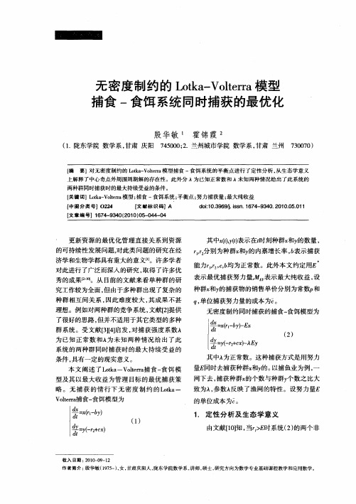
郑 影, 常 春. 基于Lotka-Volterra捕食者-猎物模型的概念间相关关系研究[J]. 中华医学图书情报杂志, 2022, 31(12): 7-13. DOI：10.3969/j.issn.1671-3982.2022.12.002·研究与探讨·基于Lotka-Volterra捕食者–猎物模型的概念间相关关系研究郑 影，常 春[摘要]目的：相关关系是叙词表中一种重要的概念关系。

对具有相关关系的概念间属性进行研究，对叙词表相关关系的构建和更新维护有重要意义。

方法：假设具有“捕食”关系的概念数量变化符合生态学中Lotka-Volterra捕食者-猎物模型，以农业领域中一个主题概念为起点，获取相关关系概念网络，在对各组相关关系进行判断之后，在中国知网（CNKI）中获取各个概念2000-2021年历年文献量，使用SPSS软件对数据进行统计分析。

结果：80%具有“捕食”关系的概念符合Lotka-Volterra捕食者-猎物模型。

结论：可通过概念间词频的关系来为叙词表的编制和维护工作提供参考建议。

[关键词]Lotka-Volterra模型；捕食关系；叙词表；概念；词频[中图分类号]G254.2；G254.0[文献标志码]A[文章编号]1671-3982(2022)12-0007-07Research on associative relationship of concepts based on Lotka-Volterra Predator-Prey ModelZHENG Ying, CHANG Chun（Institute of Scientific and Technical Information of China, Beijing 100038, China）Corresponding author: CHANG Chun[Abstract]Objective The associative relationship plays a key role in thesaurus, and the research on the attributes of concepts with associative relationship is of great significance to the construction, updating and maintenance of associative relationship in thesaurus. Methods Assuming that the variation in the number of concepts with "predator" relationship fit the Lotka-Volterra predator-prey model in ecology, the concept network of associative relationship was obtained starting from a topic concept in the agricultural field. After the associative relationship of each group was determined, the literature volume of each concept from 2000 to 2021 was obtained from CNKI, and the data were statistically analyzed by SPSS software. Results 80% of the concepts with “predator” relationship fit the Lotka-Volterra predator-prey model. Conclusion The relationship of word frequency between concepts can provide a reference for the compilation and maintenance of thesaurus.[Key words]Lotka-volterra model; Predator-prey relationship; Thesaurus; Concept; Word frequency叙词表又称为主题词表，是将自然语言转换为规范语言的一种受控的结构化词表，它概括了各门或某一学科领域知识，并由术语表达的概念及语义关系构成［1］；在文献标引与情报检索过程中，它是一种用以将文献、标引人员及用户的自然语言转换为统一的系统语言的术语控制工具［2］。

捕食者与被捕食者模型——Logistic-Volterra模型摘要Logistic模型是最常用的模型之一，在其基础上又可以发展出许多其他数学模型，其重要性不言而喻，而Volterra模型则是经典的被捕食者与捕食者模型之一。

本文尝试结合两者，建立一个Logistic-Volterra模型，并做出数值解和分析。

关键词：Logistic模型 Volterra模型数值解一、问题的提出Volterra模型显示的被捕食者与捕食者系统存在着显著的周期振荡，而实际上，多数的捕食者与捕食者系统都是观察不到的。

尝试建立模型，描述这种现象。

二、符号说明r：被捕食者固有增长率d：捕食者固有死亡率a：捕食者掠取被捕食者的能力b：被捕食者供养捕食者的能力N1：被捕食者的最大环境容纳量N2：捕食者的最大环境容纳量三、模型假设1.在没有天敌的情况下，被捕食者数量增加的固有速度与被捕食者数量x和阻滞作用因子(1-x/N1)成正比，即dxdt =rx(1−xN1)2.在没有食物的情况下，捕食者数量减少的固有速度与捕食者数量y和阻滞作用因子(1+y/N2)成正比，即dydt =−dy(1+yN2)3.捕食者与被捕食者在同一环境下生存，它们的种群变化速度互相影响，影响因子应与它们相遇的频率成正比，即捕食导致被捕食者数量减少的速度为-axy，捕食导致捕食者数量增加的速度为bxy四、模型建立与求解1.Volterra模型的分析意大利数学家Volterra在上世纪20年代提出的Volterra模型：dxdt=rx−axydydt=−dy+bxy取r=1 d=0.5 a=0.1 b=0.02，运用matlab的ode45功能函数，做出数值解，并绘图分析。

图1被捕食者与捕食者随时间变化图图2捕食者与被捕食者相图从图形可以看出，捕食者与被捕食者共同生存，数量随时间作周期变化。

2.建立Logistic-Volterra模型在Volterra模型中的物种自身增长率中，考虑自身阻滞作用，即加入Logistic项，得到以下模型：dx dt =rx(1−xN1)−axydy dt =−dy(1+yN2)+bxy取r=1 d=0.5 a=0.1 b=0.02 N1=100 N2=25，运用matlab的ode45功能函数，做出数值解，并绘图分析。

Lotka-Volterra Predator-Prey ModelsCreated by Jeff A. Tracey, PhD.Background:The interaction between predators and prey is of great interest to ecologists. In the 1920s, Alfred Lotka and Vito Volterra independently derived a pair of equations, called the Lotka-Volterra predatory-prey model, that have since been used by ecologists to describe the interactions of predators and prey. These equations, as you will see, can produce cyclical rise and fall in the abundance of predators and prey. These cycles have been observed in many predator-prey systems, including the famous example of Canadian lynx and snowshoe hares (Figure [PHOTO]). In lynx and snowshoe hare population trajectories reconstructed from trapping records (REF, Figure X), both lynx and hare numbers appear to rise and fall (cycle), with the lynx numbers beginning to decline after the number hares (their primary food source) declines.[ --- PHOTO (MAYBE) OF LYNX CAPTURING HARE --- ]This area of inquiry is even more important today as ecologists and conservation biologists consider the role of predators in ecosystems and the consequences of their extirpation. Recent research has emphasized the importance of predators in many ecosystems (for example, the reintroduction of wolves in Yellowstone National Park).The purpose of this learning module is to explore deterministic and stochastic versions of the Lotka-Volterra predator-prey equations. For a given set of initial conditions (say, the number of predators and the number of prey at the time the model begins) and model parameters, deterministic models yield the same results each time the model is run. However, we do not understand all of the processes that affect the behavior of predators and prey (or other systems), so we often include some randomness in the models to account for this uncertainty. Models that contain such randomness are called “stochastic models,” and yield different results each time they are run even if the initial conditions and parameters are the same.In this learning module, you will be able to explore deterministic and stochastic versions of four variations of the Lotka-Volterra predator-prey model using a computer program designed for this purpose.The Model:With the Lotka-Volterra predator-prey model, we model the change in the number of predators (P) and number prey (V) in continuous time via a system of two ordinary differential equations. In the equations, d V/dt represents the change in the number of prey at an instant in time, and d P/dt represents the change in the number of predators at an instant in time. Each term in the equations has a biological interpretation which I will give.The predators have a death rate (q) which controls the rate of exponential decline of the predator population (P) in the absence of prey. Prey on the other hand, have a growth rate (r) which controls the rate at which the prey population (V) grows in the absence of predators (for the exponential Models 1 and 2). With respect to prey, models 1 and 2 are “exponential models” for population growth. In models 3 and 4 we include another term, (-r/K)V2, which causes the prey growth rate to decline as the number of prey increases. This is called a “logistic model” for population growth. The logistic models include a second parameter, the carrying capacity (K), which limits the size the prey population can attain.In order for the predator population to grow, predators must consume prey. This interaction is modeled by the last term in the dV/dt equation and the first term in the d P/dt equation. This term involves a functional response, which models the rate at which predators capture and consume prey. For models 1 and 3, the functional response is aV. This is a Type I functional response in which the rate of prey capture and consumption by each predator increases linearly with the number of prey. In this model, prey are converted to predators by the first term in the dP/dt equation as bV, where b is called the “conversion efficiency.” However, it might be unrealistic to assume that there is no limit to the number of prey a predator may consume, so models 2 and 4 use a Type II functional response, in which the rate of prey capture and conversion to predators increases non-linearly with the number of prey. The formulation for each of the four Lotka-Volterra predator-prey models is:Deterministic Models: In the deterministic models, the number of prey (V) and predators (P) is treated as a continuous quantity. The program uses the equations above, initial values for V and P, and numerical methods to produce the deterministic population trajectories.Stochastic Models: In the stochastic models, the number of prey (V) and predators (P) is treated as a discrete (whole number) quantity. It is beyond the scope of this introduction to fully explain how the stochastic models work, so here I will give a brief explanation. In each of the two equations, the sum of the terms with positive signs can be thought of as the rate at which individuals are added to the population, and the sum of the absolute values of the terms with the negative signs can be thought of as the rate at which individuals are removed from the population. From these rates we determine a length of time to the next event, and which type of event occurs. The possible events are:●birth of a prey, in which case V increases by 1●death of a prey, in which case V decreases by 1●birth of a predator, in which case P increases by 1●death of a predator, in which case P decreases by 1From this process, we simulate the stochastic population trajectories. In the absence of extinction of predators or prey, the stochastic versions will, on average produce behavior similar to the deterministic models (but notice what happens if the predators become extinct).The Program:When the program is started, two windows are displayed. The first is a Control Panel (Figure 1) and the second is a Population Trajectory panel (Figure 2 and 3). The Control Panel allows you to select the version of the model to run, set all of the parameters and initial conditions for the model, the number of time steps, reset the model, run stochastic versions, and quit the program. The Population Trajectory panel displays the number of predators (in red) and prey (in blue) over time. If stochastic simulations are run (by clicking the “STOCHASTIC” button, which can be done repeatedly), the number of predators are displayed in light red and the number of prey in light blue.Figure 2: The Control Panel.Figure 3: The Population Trajectory panel displaying deterministic trajectories.Figure 4: The Population Trajectory panel displaying deterministic and stochastic trajectories.The program is started by double clicking the PredPreySim.jar file under Windows or calling the PredPreySim.sh BASH shell script from a command-line terminal in Linux or Mac OS. In order to run the program you must have the Java Virtual Machine (JVM) properly installed and on your computer's search path. If you do not have the JVM installed on your computer, you can download it for free from the Sun Microsystems website(/en/download/index.jsp).Once the program is running, deterministic predator and prey population trajectories will be displayed for the default parameters. If you change parameters, click the “RESET” button and then “RESUME.” To plot stochastic population trajectories, click the “STOCHASTIC” button.Note, however, that stochastic simulations can take a very long time for exponential models, especially for long time steps or if the prey intrinsic rate of increase is high.Exercises:Investigation 1: What happens if there are no predators? Set the predator slider to 0 and lower the time steps slider to about 20. Run each of the four models, and vary the prey rate of increase and carrying capacity.Investigation 2: Now add predators to the system. What happens to the number of prey? Explore the behavior of the model by varying the following parameters:●Model 1 – vary prey rate of increase, predator death rate, the encounter rate, andconversion efficiency.●Model 2 – vary prey rate of increase, predator death rate, the encounter rate,conversion efficiency, and prey handling time.●Model 3 – vary prey rate of increase, prey carrying capacity, predator death rate, theencounter rate, and conversion efficiency.●Model 4 – vary vary prey rate of increase, prey carrying capacity, predator death rate,the encounter rate, conversion efficiency, and prey handling time.The initial number of predators and prey can also be changed.What different behaviors are produced by the model? How do the deterministic and stochastic model results differ?Based on your explorations on one version of the model, write a 1 – 2 page description of (a) the model, (b) the basic kinds of behaviors it can produce, (c) how each of the model parameters affects the behavior of the model, and (d) the outcome of stochastic versions of the model and how they compare to the deterministic version.。

基础生态学实验实验名称Lotka-Voltena捕食者.猎物模型模拟姓名学号系别班级实验H期同组姓名［实验原理］Lotka-Volteira 捕仅者-猎物模型是 20 试剂 20 年代 Lotka A J. （1925） fD Volterra V. （1926）提出的描述种群关系的经典模型之一。

该模型假设：除捕茂者存在外，猎物生活于理想坏境中（其出生率和死亡率与密度无关）：捕ft者的环境同样是理想的，其种群增长只受到可获得的猎物数量限制。

Lotka-Volterra捕仪者-猎物模型模拟的连续增长微分方程为：dN—=r1N-C1NP(1)dP—=-r2N+C2NP (2)式中：N——猎物密度：n——猎物种群增长率：c x一甫茂者发现利进攻猎物的效率，即平均每一捕食者捕杀猎物的常数；P——Hi仪者密度：-r2—捕食者的死亡率：C2一仅考利用猎物而转变为更多捕食者的捕食常数。

方程（1）描述了猎物种群动态，倾向于r］N的无限增长，但婆受捕仅者功能项C】NP的制约。

方程（2）描述了捕食者种群动态，捕仗者数量一方面受死亡率的影响，另一方而受与猎物密度有关的数值C?NP的影响。

当模型平衡，即兽=兽=0时，P = \ , N = ?。

说明当捕仅者的数量为g时，猎物Ctt dt Cj C2 Cj数杲将稳泄不变：捕仗者嗷量大于、时，猎物的数量会减少；捕食者的数量小于务猎物数Cl C1量增加。

同样，猎物数量为孑，捕仅骨数屋也会恒定不变：猎物数量人于孑时，捕仗者数量C2 C2上升，反之捕食者数量下降。

Lotka-Volteira捕食者-猎物模型揭示了这种捕仅关系的两个种群数最动态是彼此消长、往复振荡的变化规律。

Predators0 10 30Avsuop 2 O 8 6 4 2•••o o o O807060504030 AtrsuQp Aa」dGenerationni8 in^prewavg ■S5u v> ecologists to explore thenYear兔子与獪刑的种群震荡［实验目的］1、 掌握Lotka-Volterra 捕食者-猎物模型的生态学意义与各參数意义。

lotka-volterra模型的假设全文共四篇示例，供读者参考第一篇示例：Lotka-Volterra模型是一种描述捕食者-被捕食者动态的数学模型，以其简单而有效地描述生态系统中捕食关系而闻名。

这个模型基于一系列假设，这些假设对于描述生态系统中的捕食者和被捕食者之间的相互作用至关重要。

Lotka-Volterra模型假设生态系统中只存在两种种群：捕食者和被捕食者。

捕食者是以被捕食者为食的生物，而被捕食者是被捕食者所猎食的生物。

这两种种群之间形成了一种捕食关系，即捕食者依靠捕食被捕食者来获得能量和营养。

Lotka-Volterra模型假设捕食者和被捕食者的种群数量在一定时间范围内可以被表示为连续的变量。

这意味着在任何给定的时间点上，种群数量可以通过一个数值来描述，而不是通过一系列离散的单位来描述。

这一假设是建立数学模型的基础，使得我们可以通过数学方程来描述捕食者和被捕食者之间的相互作用。

Lotka-Volterra模型假设生态系统中的其他因素对捕食者和被捕食者之间的相互作用没有直接影响。

这意味着模型中只考虑了捕食者和被捕食者之间的相互作用，而忽略了其他可能影响种群数量的因素，如环境因素、竞争关系等。

这种简化模型的做法使得我们能够更容易地研究捕食者和被捕食者之间的关系，但也可能忽略了一些现实中的复杂性。

Lotka-Volterra模型假设捕食者和被捕食者的数量是连续变化的，而且种群数量的增长速率受到食物供应和捕食压力的影响。

这种假设基于生态系统中捕食者和被捕食者之间的相互作用，捕食者的数量受到食物供应的限制，而被捕食者的数量受到捕食者的压力的限制。

这种双向的相互作用导致捕食者和被捕食者之间的数量变化呈现出周期性波动的特点。

Lotka-Volterra模型基于一系列假设来描述生态系统中捕食者和被捕食者之间的相互作用。

这些假设为我们理解生态系统中的捕食关系提供了一个简单而有效的数学框架，帮助我们研究种群数量的变化及其对生态系统稳定性的影响。