adaboost完整版

Adaboost算法的MATLAB实现：clear allclctr_n=200;%the population of the train sette_n=200;%the population of the test setweak_learner_n=20;%the population of the weak_learner tr_set=[1,5;2,3;3,2;4,6;4,7;5,9;6,5;6,7;8,5;8,8];te_se=[1,5;2,3;3,2;4,6;4,7;5,9;6,5;6,7;8,5;8,8];tr_labels=[2,2,1,1,2,2,1,2,1,1];te_labels=[2,2,1,1,2,2,1,2,1,1];figure;subplot(2,2,1);hold on;axis square;indices=tr_labels==1;plot(tr_set(indices,1),tr_set(indices,2),'b*');indices=~indices;plot(tr_set(indices,1),tr_set(indices,2),'r*');title('Training set');subplot(2,2,2);hold on;axis square;indices=te_labels==1;plot(te_set(indices,1),te_set(indices,2),'b*')3;indices=~indices;plot(te_set(indices,1),te_set(indices,2),'r*');title('Training set');%Training and testing error ratestr_error=zeros(1,weak_learner_n);te_error=zeros(1,weak_learner_n);for i=1:weak_learner_nadaboost_model=adaboost_tr(@threshold_tr,@threshold_te,tr_set,tr_labels,i); [L_tr,hits_tr]=adaboost_te(adaboost_model,@threshold_te,te_set,te_labels); tr_error(i)=(tr_n-hits_tr)/tr_n;[L_te,hits_te]=adaboost_te(adaboost_model,@threshold_te,te_set,te_labels); te_error(i)=(te_n-hits_te)/te_n;endsubplot(2,2,3);plot(1:weak_learner_n,tr_error);axis([1,weak_learner_n,0,1]);title('Training Error');xlabel('weak classifier number');ylabel('error rate');grid on;subplot(2,2,4);axis square;plot(1:weak_learner_n,te_error);axis([1,weak_learner_n,0,1]);title('Testing Error');xlabel('weak classifier number');ylabel('error rate');grid on;这里需要另外分别撰写两个函数，其中一个为生成adaboost模型的训练函数，另外为测试测试样本的测试函数。

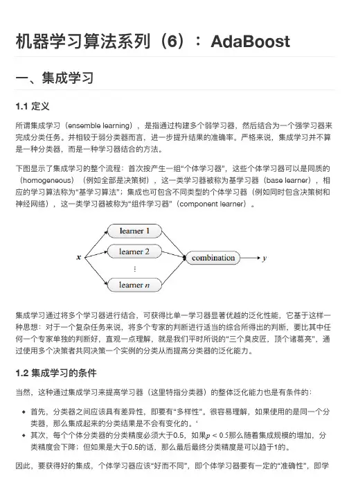
AdaBoost装袋提升算法参开资料：更多挖掘算法：介绍在介绍AdaBoost算法之前，需要了解⼀个类似的算法，装袋算法(bagging)，bagging是⼀种提⾼分类准确率的算法，通过给定组合投票的⽅式，获得最优解。

⽐如你⽣病了，去n个医院看了n个医⽣，每个医⽣给你开了药⽅，最后的结果中，哪个药⽅的出现的次数多，那就说明这个药⽅就越有可能性是最由解，这个很好理解。

⽽bagging算法就是这个思想。

算法原理⽽AdaBoost算法的核⼼思想还是基于bagging算法，但是他⼜⼀点点的改进，上⾯的每个医⽣的投票结果都是⼀样的，说明地位平等，如果在这⾥加上⼀个权重，⼤城市的医⽣权重⾼点，⼩县城的医⽣权重低，这样通过最终计算权重和的⽅式，会更加的合理，这就是AdaBoost算法。

AdaBoost算法是⼀种迭代算法，只有最终分类误差率⼩于阈值算法才能停⽌，针对同⼀训练集数据训练不同的分类器，我们称弱分类器，最后按照权重和的形式组合起来，构成⼀个组合分类器，就是⼀个强分类器了。

算法的只要过程：1、对D训练集数据训练处⼀个分类器Ci2、通过分类器Ci对数据进⾏分类，计算此时误差率3、把上步骤中的分错的数据的权重提⾼，分对的权重降低，以此凸显了分错的数据。

为什么这么做呢，后⾯会做出解释。

完整的adaboost算法如下最后的sign函数是符号函数，如果最后的值为正，则分为+1类，否则即使-1类。

我们举个例⼦代⼊上⾯的过程，这样能够更好的理解。

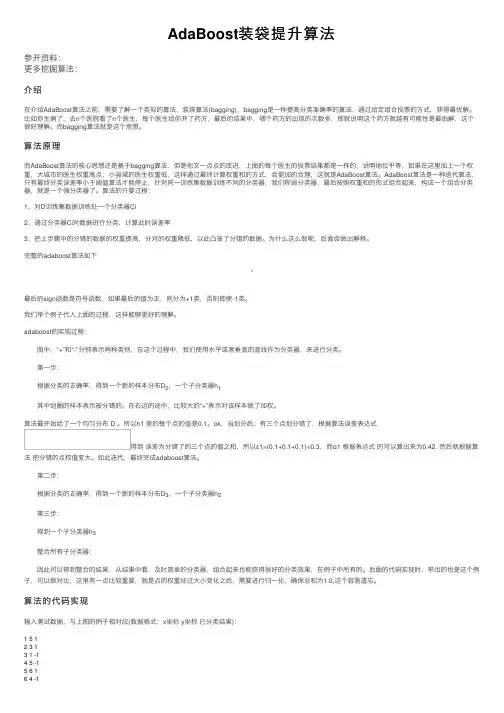
adaboost的实现过程： 图中，“+”和“-”分别表⽰两种类别，在这个过程中，我们使⽤⽔平或者垂直的直线作为分类器，来进⾏分类。

第⼀步： 根据分类的正确率，得到⼀个新的样本分布D2，⼀个⼦分类器h1 其中划圈的样本表⽰被分错的。

在右边的途中，⽐较⼤的“+”表⽰对该样本做了加权。

算法最开始给了⼀个均匀分布 D 。

所以h1 ⾥的每个点的值是0.1。

ok，当划分后，有三个点划分错了，根据算法误差表达式得到误差为分错了的三个点的值之和，所以ɛ1=(0.1+0.1+0.1)=0.3，⽽ɑ1 根据表达式的可以算出来为0.42. 然后就根据算法把分错的点权值变⼤。

数据挖掘领域⼗⼤经典算法之—AdaBoost算法（超详细附代码）相关⽂章：数据挖掘领域⼗⼤经典算法之—C4.5算法（超详细附代码）数据挖掘领域⼗⼤经典算法之—K-Means算法（超详细附代码）数据挖掘领域⼗⼤经典算法之—SVM算法（超详细附代码）数据挖掘领域⼗⼤经典算法之—Apriori算法数据挖掘领域⼗⼤经典算法之—EM算法数据挖掘领域⼗⼤经典算法之—PageRank算法数据挖掘领域⼗⼤经典算法之—K-邻近算法/kNN（超详细附代码）数据挖掘领域⼗⼤经典算法之—朴素贝叶斯算法（超详细附代码）数据挖掘领域⼗⼤经典算法之—CART算法（超详细附代码）简介Adaboost算法是⼀种提升⽅法，将多个弱分类器，组合成强分类器。

AdaBoost，是英⽂”Adaptive Boosting“（⾃适应增强）的缩写，由Yoav Freund和Robert Schapire在1995年提出。

它的⾃适应在于：前⼀个弱分类器分错的样本的权值（样本对应的权值）会得到加强，权值更新后的样本再次被⽤来训练下⼀个新的弱分类器。

在每轮训练中，⽤总体（样本总体）训练新的弱分类器，产⽣新的样本权值、该弱分类器的话语权，⼀直迭代直到达到预定的错误率或达到指定的最⼤迭代次数。

总体——样本——个体三者间的关系需要搞清除总体N。

样本：｛ni｝i从1到M。

个体：如n1=（1,2），样本n1中有两个个体。

算法原理（1）初始化训练数据（每个样本）的权值分布：如果有N个样本，则每⼀个训练的样本点最开始时都被赋予相同的权重：1/N。

（2）训练弱分类器。

具体训练过程中，如果某个样本已经被准确地分类，那么在构造下⼀个训练集中，它的权重就被降低；相反，如果某个样本点没有被准确地分类，那么它的权重就得到提⾼。

同时，得到弱分类器对应的话语权。

然后，更新权值后的样本集被⽤于训练下⼀个分类器，整个训练过程如此迭代地进⾏下去。

（3）将各个训练得到的弱分类器组合成强分类器。

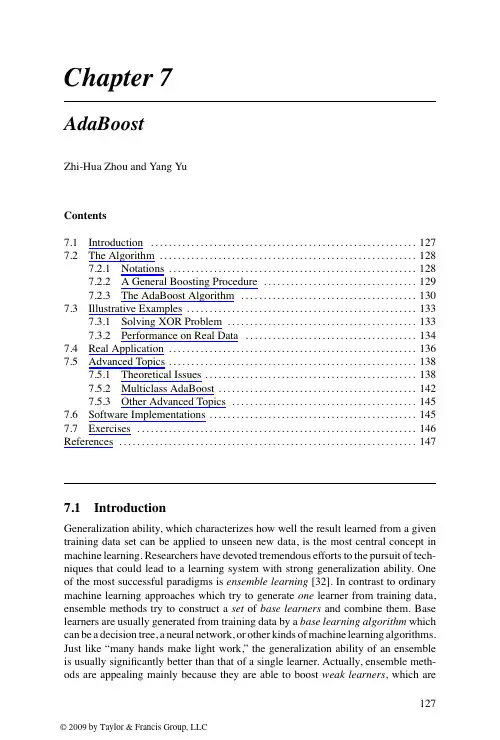
Chapter7AdaBoostZhi-Hua Zhou and Yang YuContents7.1Introduction (127)7.2The Algorithm (128)7.2.1Notations (128)7.2.2A General Boosting Procedure (129)7.2.3The AdaBoost Algorithm (130)7.3Illustrative Examples (133)7.3.1Solving XOR Problem (133)7.3.2Performance on Real Data (134)7.4Real Application (136)7.5Advanced Topics (138)7.5.1Theoretical Issues (138)7.5.2Multiclass AdaBoost (142)7.5.3Other Advanced Topics (145)7.6Software Implementations (145)7.7Exercises (146)References (147)7.1IntroductionGeneralization ability,which characterizes how well the result learned from a given training data set can be applied to unseen new data,is the most central concept in machine learning.Researchers have devoted tremendous efforts to the pursuit of tech-niques that could lead to a learning system with strong generalization ability.One of the most successful paradigms is ensemble learning[32].In contrast to ordinary machine learning approaches which try to generate one learner from training data, ensemble methods try to construct a set of base learners and combine them.Base learners are usually generated from training data by a base learning algorithm which can be a decision tree,a neural network,or other kinds of machine learning algorithms. Just like“many hands make light work,”the generalization ability of an ensemble is usually significantly better than that of a single learner.Actually,ensemble meth-ods are appealing mainly because they are able to boost weak learners,which are127128AdaBoostslightly better than random guess,to strong learners,which can make very accurate predictions.So,“base learners”are also referred as“weak learners.”AdaBoost[9,10]is one of the most influential ensemble methods.It took birth from the answer to an interesting question posed by Kearns and Valiant in1988.That is,whether two complexity classes,weakly learnable and strongly learnable prob-lems,are equal.If the answer to the question is positive,a weak learner that performs just slightly better than random guess can be“boosted”into an arbitrarily accurate strong learner.Obviously,such a question is of great importance to machine learning. Schapire[21]found that the answer to the question is“yes,”and gave a proof by construction,which is thefirst boosting algorithm.An important practical deficiency of this algorithm is the requirement that the error bound of the base learners be known ahead of time,which is usually unknown in practice.Freund and Schapire[9]then pro-posed an adaptive boosting algorithm,named AdaBoost,which does not require those unavailable information.It is evident that AdaBoost was born with theoretical signif-icance,which has given rise to abundant research on theoretical aspects of ensemble methods in communities of machine learning and statistics.It is worth mentioning that for their AdaBoost paper[9],Schapire and Freund won the Godel Prize,which is one of the most prestigious awards in theoretical computer science,in the year2003. AdaBoost and its variants have been applied to diverse domains with great success, owing to their solid theoretical foundation,accurate prediction,and great simplicity (Schapire said it needs only“just10lines of code”).For example,Viola and Jones[27] combined AdaBoost with a cascade process for face detection.They regarded rectan-gular features as weak learners,and by using AdaBoost to weight the weak learners, they got very intuitive features for face detection.In order to get high accuracy as well as high efficiency,they used a cascade process(which is beyond the scope of this chap-ter).As a result,they reported a very strong face detector:On a466MHz machine,face detection on a384×288image costs only0.067second,which is15times faster than state-of-the-art face detectors at that time but with comparable accuracy.This face detector has been recognized as one of the most exciting breakthroughs in computer vision(in particular,face detection)during the past decade.It is not strange that“boost-ing”has become a buzzword in computer vision and many other application areas. In the rest of this chapter,we will introduce the algorithm and implementations,and give some illustrations on how the algorithm works.For readers who are eager to know more,we will introduce some theoretical results and extensions as advanced topics.7.2The Algorithm7.2.1NotationsWefirst introduce some notations that will be used in the rest of the chapter.Let X denote the instance space,or in other words,feature space.Let Y denote the set of labels that express the underlying concepts which are to be learned.For example,we7.2The Algorithm129 let Y={−1,+1}for binary classification.A training set D consists of m instances whose associated labels are observed,i.e.,D={(x i,y i)}(i∈{1,...,m}),while the label of a test instance is unknown and thus to be predicted.We assume both training and test instances are drawn independently and identically from an underlying distribution D.After training on a training data set D,a learning algorithm L will output a hypoth-esis h,which is a mapping from X to Y,or called as a classifier.The learning process can be regarded as picking the best hypothesis from a hypothesis space,where the word“best”refers to a loss function.For classification,the loss function can naturally be0/1-loss,loss0/1(h|x)=I[h(x)=y]where I[·]is the indication function which outputs1if the inner expression is true and0otherwise,which means that one error is counted if an instance is wrongly classified.In this chapter0/1-loss is used by default,but it is noteworthy that other kinds of loss functions can also be used in boosting.7.2.2A General Boosting ProcedureBoosting is actually a family of algorithms,among which the AdaBoost algorithm is the most influential one.So,it may be easier by starting from a general boosting procedure.Suppose we are dealing with a binary classification problem,that is,we are trying to classify instances as positive and ually we assume that there exists an unknown target concept,which correctly assigns“positive”labels to instances belonging to the concept and“negative”labels to others.This unknown target concept is actually what we want to learn.We call this target concept ground-truth.For a binary classification problem,a classifier working by random guess will have50%0/1-loss. Suppose we are unlucky and only have a weak classifier at hand,which is only slightly better than random guess on the underlying instance distribution D,say,it has49%0/1-loss.Let’s denote this weak classifier as h1.It is obvious that h1is not what we want,and we will try to improve it.A natural idea is to correct the mistakes made by h1.We can try to derive a new distribution D from D,which makes the mistakes of h1more evident,for example,it focuses more on the instances wrongly classified by h1(we will explain how to generate D in the next section).We can train a classifier h2from D .Again,suppose we are unlucky and h2is also a weak classifier.Since D was derived from D,if D satisfies some condition,h2will be able to achieve a better performance than h1on some places in D where h1does not work well, without scarifying the places where h1performs well.Thus,by combining h1and h2in an appropriate way(we will explain how to combine them in the next section), the combined classifier will be able to achieve less loss than that achieved by h1.By repeating the above process,we can expect to get a combined classifier which has very small(ideally,zero)0/1-loss on D.130AdaBoostInput: Instance distribution D ; Base learning algorithm L ;Number of learning rounds T .Process:1. D 1 = D . % Initialize distribution2. for t = 1, ··· ,T :3. h t = L (D t ); % Train a weak learner from distribution D t4. єt = Pr x ~D t ,y I [h t (x )≠ y ]; % Measure the error of h t5. D t +1 = AdjustDistribution (D t , єt )6. endOutput: H (x ) = CombineOutputs ({h t (x )})Figure 7.1A general boosting procedure.Briefly,boosting works by training a set of classifiers sequentially and combining them for prediction,where the later classifiers focus more on the mistakes of the earlier classifiers.Figure 7.1summarizes the general boosting procedure.7.2.3The AdaBoost AlgorithmFigure 7.1is not a real algorithm since there are some undecided parts such as Ad just Distribution and CombineOutputs .The AdaBoost algorithm can be viewed as an instantiation of the general boosting procedure,which is summarized in Figure 7.2.Input: Data set D = {(x 1, y 1), (x 2, y 2), . . . , (x m , y m )};Base learning algorithm L ;Number of learning rounds T .Process:1. D 1 (i ) = 1/m . % Initialize the weight distribution2. for t = 1, ··· ,T :3. h t = L (D , D t ); % Train a learner h t from D using distribution D t4. єt = Pr x ~D t ,y I [h t (x )≠ y ]; % Measure the error of h t5. if єt > 0.5 then break6. αt = ½ ln ( ); % Determine the weight of h t7. D t +1 (i ) =8. endOutput: H (x ) = sign (Σt =1αt h t (x ))× {exp(–αt ) if h t (x i ) = y i exp(αt ) if h t (x i ) ≠ y i % Update the distribution, where % Z t is a normalization factor which% enables D t +1 to be distribution T 1– єt єt D t (i )Z t D t (i )exp(–αt y i h t (x i ))Z t Figure 7.2The AdaBoost algorithm.7.2The Algorithm 131Now we explain the details.1AdaBoost generates a sequence of hypotheses and combines them with weights,which can be regarded as an additive weighted combi-nation in the form of H (x )=T t =1αt h t (x )From this view,AdaBoost actually solves two problems,that is,how to generate the hypotheses h t ’s and how to determine the proper weights αt ’s.In order to have a highly efficient error reduction process,we try to minimize an exponential lossloss exp (h )=E x ∼D ,y [e −yh (x )]where yh (x )is called as the classification margin of the hypothesis.Let’s consider one round in the boosting process.Suppose a set of hypotheses as well as their weights have already been obtained,and let H denote the combined hypothesis.Now,one more hypothesis h will be generated and is to be combined with H to form H +αh .The loss after the combination will beloss exp (H +αh )=E x ∼D ,y [e −y (H (x )+αh (x ))]The loss can be decomposed to each instance,which is called pointwise loss,asloss exp (H +αh |x )=E y [e −y (H (x )+αh (x ))|x ]Since y and h (x )must be +1or −1,we can expand the expectation as loss exp (H +αh |x )=e −y H (x ) e −αP (y =h (x )|x )+e αP (y =h (x )|x ) Suppose we have already generated h ,and thus the weight αthat minimizes the loss can be found when the derivative of the loss equals zero,that is,∂loss exp (H +αh |x )∂α=e −y H (x ) −e −αP (y =h (x )|x )+e αP (y =h (x )|x ) =0and the solution isα=12ln P (y =h (x )|x )P (y =h (x )|x )=12ln 1−P (y =h (x )|x )P (y =h (x )|x )By taking an expectation over x ,that is,solving∂loss exp (H +αh )∂α=0,and denoting=E x ∼D [y =h (x )],we getα=12ln 1− which is the way of determining αt in AdaBoost.1Here we explain the AdaBoost algorithm from the view of [11]since it is easier to understand than the original explanation in [9].132AdaBoostNow let’s consider how to generate h.Given a base learning algorithm,AdaBoost invokes it to produce a hypothesis from a particular instance distribution.So,we only need to consider what hypothesis is desired for the next round,and then generate an instance distribution to achieve this hypothesis.We can expand the pointwise loss to second order about h(x)=0,whenfixing α=1,loss exp(H+h|x)≈E y[e−y H(x)(1−yh(x)+y2h(x)2/2)|x]=E y[e−y H(x)(1−yh(x)+1/2)|x]since y2=1and h(x)2=1.Then a perfect hypothesis ish∗(x)=arg minh loss exp(H+h|x)=arg maxhE y[e−y H(x)yh(x)|x]=arg maxhe−H(x)P(y=1|x)·1·h(x)+e H(x)P(y=−1|x)·(−1)·h(x) Note that e−y H(x)is a constant in terms of h(x).By normalizing the expectation ash∗(x)=arg maxh e−H(x)P(y=1|x)·1·h(x)+e H(x)P(y=−1|x)·(−1)·h(x)e P(y=1|x)+e P(y=−1|x)we can rewrite the expectation using a new term w(x,y),which is drawn from e−y H(x)P(y|x),ash∗(x)=arg maxhE w(x,y)∼e−y H(x)P(y|x)[yh(x)|x]Since h∗(x)must be+1or−1,the solution to the optimization is that h∗(x)holds the same sign with y|x,that is,h∗(x)=E w(x,y)∼e−y H(x)P(y|x)[y|x]=P w(x,y)∼e−y H(x)P(y|x)(y=1|x)−P w(x,y)∼e−y H(x)P(y|x)(y=−1|x)As can be seen,h∗simply performs the optimal classification of x under the distri-bution e−y H(x)P(y|x).Therefore,e−y H(x)P(y|x)is the desired distribution for a hypothesis minimizing0/1-loss.So,when the hypothesis h(x)has been learned andα=12ln1−has been deter-mined in the current round,the distribution for the next round should beD t+1(x)=e−y(H(x)+αh(x))P(y|x)=e−y H(x)P(y|x)·e−αyh(x)=D t(x)·e−αyh(x)which is the way of updating instance distribution in AdaBoost.But,why optimizing the exponential loss works for minimizing the0/1-loss? Actually,we can see thath∗(x)=arg minh E x∼D,y[e−yh(x)|x]=12lnP(y=1|x)P(y=−1|x)7.3Illustrative Examples133 and therefore we havesign(h∗(x))=arg maxyP(y|x)which implies that the optimal solution to the exponential loss achieves the minimum Bayesian error for the classification problem.Moreover,we can see that the function h∗which minimizes the exponential loss is the logistic regression model up to a factor 2.So,by ignoring the factor1/2,AdaBoost can also be viewed asfitting an additive logistic regression model.It is noteworthy that the data distribution is not known in practice,and the AdaBoost algorithm works on a given training set withfinite training examples.Therefore,all the expectations in the above derivations are taken on the training examples,and the weights are also imposed on training examples.For base learning algorithms that cannot handle weighted training examples,a resampling mechanism,which samples training examples according to desired weights,can be used instead.7.3Illustrative ExamplesIn this section,we demonstrate how the AdaBoost algorithm works,from an illustra-tion on a toy problem to real data sets.7.3.1Solving XOR ProblemWe consider an artificial data set in a two-dimensional space,plotted in Figure7.3(a). There are only four instances,that is,⎧⎪⎪⎪⎨⎪⎪⎪⎩(x1=(0,+1),y1=+1) (x2=(0,−1),y2=+1) (x3=(+1,0),y3=−1) (x4=(−1,0),y4=−1)⎫⎪⎪⎪⎬⎪⎪⎪⎭This is the XOR problem.The two classes cannot be separated by a linear classifier which corresponds to a line on thefigure.Suppose we have a base learning algorithm which tries to select the best of the fol-lowing eight functions.Note that none of them is perfect.For equally good functions, the base learning algorithm will pick one function from them randomly.h1(x)=+1,if(x1>−0.5)−1,otherwise h2(x)=−1,if(x1>−0.5)+1,otherwiseh3(x)=+1,if(x1>+0.5)−1,otherwise h4(x)=−1,if(x1>+0.5)+1,otherwise134AdaBoost(a) The XOR data(b) 1st round(c) 2nd round(d) 3rd round Figure7.3AdaBoost on the XOR problem.h5(x)=+1,if(x2>−0.5)−1,otherwise h6(x)=−1,if(x2>−0.5)+1,otherwiseh7(x)=+1,if(x2>+0.5)−1,otherwise h8(x)=−1,if(x2>+0.5)+1,otherwisewhere x1and x2are the values of x at thefirst and second dimension,respectively. Now we track how AdaBoost works:1.Thefirst step is to invoke the base learning algorithm on the original data.h2,h3,h5,and h8all have0.25classification errors.Suppose h2is picked as thefirst base learner.One instance,x1,is wrongly classified,so the error is1/4=0.25.The weight of h2is0.5ln3≈0.55.Figure7.3(b)visualizes the classification, where the shadowed area is classified as negative(−1)and the weights of the classification,0.55and−0.55,are displayed.2.The weight of x1is increased and the base learning algorithm is invoked again.This time h3,h5,and h8have equal errors.Suppose h3is picked,of which the weight is0.80.Figure7.3(c)shows the combined classification of h2and h3with their weights,where different gray levels are used for distinguishing negative areas according to classification weights.3.The weight of x3is increased,and this time only h5and h8equally have thelowest errors.Suppose h5is picked,of which the weight is1.10.Figure7.3(d) shows the combined classification of h2,h3,and h8.If we look at the sign of classification weights in each area in Figure7.3(d),all the instances are correctly classified.Thus,by combining the imperfect linear classifiers,AdaBoost has produced a nonlinear classifier which has zero error.7.3.2Performance on Real DataWe evaluate the AdaBoost algorithm on56data sets from the UCI Machine Learning Repository,2which covers a broad range of real-world tasks.We use the Weka(will be introduced in Section7.6)implementation of AdaBoost.M1using reweighting with /∼mlearn/MLRepository.html7.3Illustrative Examples 135AdaBoost with decision tree (unpruned)AdaBoost with decision tree (pruned)AdaBoost with decision stumpD e c i s i o n s t u m p D e c i s i o n t r e e (p r u n e d )1.000.800.600.400.200.00 1.000.800.600.400.200.000.000.200.400.600.80 1.000.000.200.400.600.80 1.00D e c i s i o n t r e e (u n p r u n e d )1.000.800.600.400.200.000.000.200.400.600.80 1.00Figure 7.4Comparison of predictive errors of AdaBoost against decision stump,pruned,and unpruned single decision trees on 56UCI data sets.50base learners.Almost all kinds of learning algorithms can be taken as base learning algorithms,such as decision trees,neural networks,and so on.Here,we have tried three base learning algorithms,including decision stump,pruned,and unpruned J4.8decision trees (Weka implementation of C4.5).We plot the comparison results in Figure 7.4,where each circle represents a data set and locates according to the predictive errors of the two compared algorithms.In each plot of Figure 7.4,the diagonal line indicates where the two compared algorithms have identical errors.It can be observed that AdaBoost often outperforms its base learning algorithm,with a few exceptions on which it degenerates the performance.The famous bias-variance decomposition [12]has been employed to empirically study why AdaBoost achieves excellent performance [2,3,34].This powerful tool breaks the expected error of a learning approach into the sum of three nonnegative quantities,that is,the intrinsic noise,the bias,and the variance.The bias measures how closely the average estimate of the learning approach is able to approximate the target,and the variance measures how much the estimate of the learning approach fluctuates for the different training sets of the same size.It has been observed [2,3,34]that AdaBoost primarily reduces the bias but it is also able to reduce the variance.136AdaBoostFigure7.5Four feature masks to be applied to each rectangle.7.4Real ApplicationViola and Jones[27]combined AdaBoost with a cascade process for face detection. As the result,they reported that on a466MHz machine,face detection on a384×288 image costs only0.067seconds,which is almost15times faster than state-of-the-art face detectors at that time but with comparable accuracy.This face detector has been recognized as one of the most exciting breakthroughs in computer vision(in particular,face detection)during the past decade.In this section,we briefly introduce how AdaBoost works in the Viola-Jones face detector.Here the task is to locate all possible human faces in a given image.An image is first divided into subimages,say24×24squares.Each subimage is then represented by a feature vector.To make the computational process efficient,very simple features are used.All possible rectangles in a subimage are examined.On every rectangle, four features are extracted using the masks shown in Figure7.5.With each mask, the sum of pixels’gray level in white areas is subtracted by the sum of those in dark areas,which is regarded as a feature.Thus,by a24×24splitting,there are more than 1million features,but each of the features can be calculated very fast.Each feature is regarded as a weak learner,that is,h i,p,θ(x)=I[px i≤pθ](p∈{+1,−1})where x i is the value of x at the i-th feature.The base learning algorithm tries tofind the best weak classifier h i∗,p∗,θ∗that minimizes the classification error,that is,E(x,y)I[h i,p,θ(x)=y](i∗,p∗,θ∗)=arg mini,p,θFace rectangles are regarded as positive examples,as shown in Figure7.6,while rectangles that do not contain any face are regarded as negative examples.Then,the AdaBoost process is applied and it will return a few weak learners,each corresponds to one of the over1million features.Actually,the AdaBoost process can be regarded as a feature selection tool here.Figure7.7shows thefirst two selected features and their position relative to a human face.It is evident that these two features are intuitive,where thefirst feature measures how the intensity of the eye areas differ from that of the lower areas,while7.4Real Application137Figure7.6Positive training examples[27].the second feature measures how the intensity of the two eye areas differ from the area between two eyes.Using the selected features in order,an extremely imbalanced decision tree is built, which is called cascade of classifiers,as illustrated in Figure7.8.The parameterθis adjusted in the cascade such that,at each tree node,branching into“not a face”means that the image is really not a face.In other words,the false negative rate is minimized.This design owes to the fact that a nonface image is easier to be recognized,and it is possible to use a few features tofilter out a lot of candidate image rectangles,which endows the high efficiency.It was reported[27]that10 features per subimage are examined in average.Some test results of the Viola-Jones face detector are shown in Figure7.9.138AdaBoost7.5Advanced Topics7.5.1Theoretical IssuesComputational learning theory studies some fundamental theoretical issues of machine learning.First introduced by Valiant in1984[25],the Probably Approx-imately Correct(PAC)framework models learning algorithms in a distribution free manner.Roughly speaking,for binary classification,a problem is learnable or stronglytimelearnable if there exists an algorithm that outputs a hypothesis h in polynomial7.5Advanced Topics139Figure7.9Outputs of the Viola-Jones face detector on a number of test images[27]. such that for all0<δ, ≤0.5,PE x∼D,y[I[h(x)=y]]<≥1−δand a problem is weakly learnable if the above holds for all0<δ≤0.5but only when is slightly smaller than0.5(or in other words,h is only slightly better than random guess).In1988,Kearns and Valiant[15]posed an interesting question,that is,whether the strongly learnable problem class equals the weakly learnable problem class.This question is of fundamental importance,since if the answer is“yes,”any weak learner is potentially able to be boosted to a strong learner.In1989,Schapire[21]proved that the answer is really“yes,”and the proof he gave is a construction,which is thefirst140AdaBoostboosting algorithm.One year later,Freund[7]developed a more efficient algorithm. Both algorithms,however,suffered from the practical deficiency that the error bound of the base learners need to be known ahead of time,which is usually unknown in ter,in1995,Freund and Schapire[9]developed the AdaBoost algorithm, which is effective and efficient in practice.Freund and Schapire[9]proved that,if the base learners of AdaBoost have errors 1, 2,···, T,the error of thefinal combined learner, ,is upper bounded as=E x∼D,y I[H(x)=y]≤2TTt=1t t≤e−2Tt=1γ2twhereγt=0.5− t.It can be seen that AdaBoost reduces the error exponentially fast.Also,it can be derived that,to achieve an error less than ,the round T is upperbounded asT≤12γln1where it is assumed thatγ=γ1=γ2=···=γT.In practice,however,all the operations of AdaBoost can only be carried out on training data D,that is,D=E x∼D,y I[H(x)=y]and thus the errors are training errors,while the generalization error,that is,the error over instance distribution DD=E x∼D,y I[H(x)=y]is of more interest.The initial analysis[9]showed that the generalization error of AdaBoost is upperbounded asD≤ D+˜OdTmwith probability at least1−δ,where d is the VC-dimension of base learners,m is the number of training instances,and˜O(·)is used instead of O(·)to hide logarithmic terms and constant factors.The above bound suggests that in order to achieve a good generalization ability, it is necessary to constrain the complexity of base learners as well as the number of learning rounds;otherwise AdaBoost will overfit.However,empirical studies show that AdaBoost often does not overfit,that is,its test error often tends to decrease even after the training error reaches zero,even after a large number of rounds,such as 1000.For example,Schapire et al.[22]plotted the performance of AdaBoost on the letter data set from UCI Machine Learning Repository,as shown in Figure7.10(left), where the higher curve is test error while the lower one is training error.It can be observed that AdaBoost achieves zero training error in less than10rounds but the generalization error keeps on reducing.This phenomenon seems to counter Occam’s7.5Advanced Topics 141e r r o r r a t e r a t i o of t e s t s e t t θ20151050 1.00.5101001000-1-0.50.51Figure 7.10Training and test error (left)and margin distribution (right)of AdaBoost on the letter data set [22].Razor,that is,nothing more than necessary should be done,which is one of the basic principles in machine learning.Many researchers have studied this phenomena,and several theoretical explana-tions have been given,for example,[11].Schapire et al.[22]introduced the margin -based explanation.They argued that AdaBoost is able to increase the margin even after the training error reaches zero,and thus it does not overfit even after a large number of rounds.The classification margin of h on x is defined as yh (x ),and that of H (x )= T t =1αt h t (x )is defined asy H (x )= Tt =1αt yh t (x ) Tt =1αtFigure 7.10(right)plots the distribution of y H (x )≤θfor different values of θ.It was proved in [22]that the generalization error is upper bounded asD ≤P x ∼D ,y (y H (x )≤θ)+˜O d m θ2+ln 1δ ≤2TT t =1 1−θt (1− )1+θ+˜O m θ2+ln δ with probability at least 1−δ.This bound qualitatively explains that when other variables in the bound are fixed,the larger the margin,the smaller the generalization error.However,this margin-based explanation was challenged by Brieman [4].Using minimum margin ,=min x ∈Dy H (x )Breiman proved a generalization error bound is tighter than the above one using minimum margin.Motivated by the tighter bound,the arc-gv algorithm,which is a variant of AdaBoost,was proposed to maximize the minimum margin directly,by142AdaBoost updatingαt according toαt=12ln1+γt1−γt−12ln1+ t1− tInterestingly,the minimum margin of arc-gv is uniformly better than that of AdaBoost, but the test error of arc-gv increases drastically on all tested data sets[4].Thus,the margin theory for AdaBoost was almost sentenced to death.In2006,Reyzin and Schapire[20]reported an interestingfinding.It is well-known that the bound of the generalization error is associated with margin,the number of rounds,and the complexity of base learners.When comparing arc-gv with AdaBoost, Breiman[4]tried to control the complexity of base learners by using decision trees with the same number of leaves,but Reyzin and Schapire found that these are trees with very different shapes.The trees generated by arc-gv tend to have larger depth, while those generated by AdaBoost tend to have larger width.Figure7.11(top) shows the difference of depth of the trees generated by the two algorithms on the breast cancer data set from UCI Machine Learning Repository.Although the trees have the same number of leaves,it seems that a deeper tree makes more attribute tests than a wider tree,and therefore they are unlikely to have equal complexity. So,Reyzin and Schapire repeated Breiman’s experiments by using decision stump, which has only one leaf and therefore is with afixed complexity,and found that the margin distribution of AdaBoost is actually better than that of arc-gv,as illustrated in Figure7.11(bottom).Recently,Wang et al.[28]introduced equilibrium margin and proved a new bound tighter than that obtained by using minimum margin,which suggests that the mini-mum margin may not be crucial for the generalization error of AdaBoost.It will be interesting to develop an algorithm that maximizes equilibrium margin directly,and to see whether the test error of such an algorithm is smaller than that of AdaBoost, which remains an open problem.7.5.2Multiclass AdaBoostIn the previous sections we focused on AdaBoost for binary classification,that is, Y={+1,−1}.In many classification tasks,however,an instance belongs to one of many instead of two classes.For example,a handwritten number belongs to1of10 classes,that is,Y={0,...,9}.There is more than one way to deal with a multiclass classification problem.AdaBoost.M1[9]is a very direct extension,which is as same as the algorithm shown in Figure7.2,except that now the base learners are multiclass learners instead of binary classifiers.This algorithm could not use binary base classifiers,and requires every base learner have less than1/2multiclass0/1-loss,which is an overstrong constraint. SAMME[35]is an improvement over AdaBoost.M1,which replaces Line5of AdaBoost.M1in Figure7.2byαt=12ln1− tt+ln(|Y|−1)。

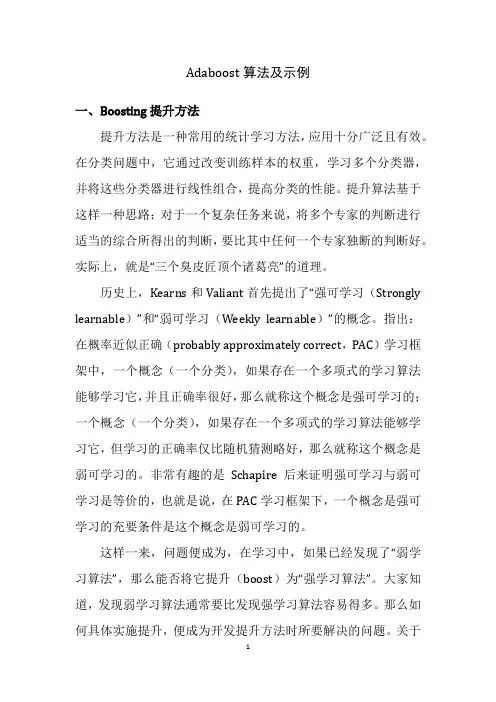
Adaboost算法及示例一、Boosting提升方法提升方法是一种常用的统计学习方法，应用十分广泛且有效。

在分类问题中，它通过改变训练样本的权重，学习多个分类器，并将这些分类器进行线性组合，提高分类的性能。

提升算法基于这样一种思路：对于一个复杂任务来说，将多个专家的判断进行适当的综合所得出的判断，要比其中任何一个专家独断的判断好。

实际上，就是“三个臭皮匠顶个诸葛亮”的道理。

历史上，Kearns和Valiant首先提出了“强可学习（Strongly learnable）”和“弱可学习（Weekly learnable）”的概念。

指出：在概率近似正确（probably approximately correct，PAC）学习框架中，一个概念（一个分类），如果存在一个多项式的学习算法能够学习它，并且正确率很好，那么就称这个概念是强可学习的；一个概念（一个分类），如果存在一个多项式的学习算法能够学习它，但学习的正确率仅比随机猜测略好，那么就称这个概念是弱可学习的。

非常有趣的是Schapire后来证明强可学习与弱可学习是等价的，也就是说，在PAC学习框架下，一个概念是强可学习的充要条件是这个概念是弱可学习的。

这样一来，问题便成为，在学习中，如果已经发现了“弱学习算法”，那么能否将它提升（boost）为“强学习算法”。

大家知道，发现弱学习算法通常要比发现强学习算法容易得多。

那么如何具体实施提升，便成为开发提升方法时所要解决的问题。

关于提升方法的研究很多，有很多算法被提出，最具代表性的是AdaBoost算法（Adaboost algorithm）。

对与分类问题而言，给定一个训练样本集，求比较粗糙的分类规则（弱分类器）要比求精确的分类规则（强分类器）容易得多。

提升方法就是从弱学习算法出发，反复学习，得到一系列分类器，然后组合这些分类器，构成一个强分类器。

这样，对于提升算法来说，有两个问题需要回答：一是在每一轮如何改变训练数据的权值分布；二是如何将弱分类器组合成一个强分类器。