美国大学生数学建模比赛的论文格式

数学建模论文格式细节各种内容均不宜直接修改格式而应修改其对应的样式；一般不宜设置左右缩进；文中不能包含任何空行；所有自动编号内容在添加或删除部分内容后无需手动维护其编号（选定所需修改编号的内容或者全文后按F9功能键）；1.摘要“摘要”作为一级标题但不参加编号；全国赛摘要中应包含关键词，“关键词”三字应该用黑体；美国赛不用写关键词；摘要后面用分页符来与后面正文分开，而非使用空行；2.各级标题同一级别的标题必须使用相同的样式，其格式的修改只能直接修改样式而不能针对某个具体的标题直接进行修改；各级标题后面不可跟标点符号；标题的标号：全国赛论文建议采用学术论文的标号，即1、2、3、1.1、1.2、1.2.3等，标号后面可以再跟小园点，亦可不跟，另外再用相同数量的空格隔开；亦可使用一、二、三等标号一级标题。

美国赛论文中通常未使用标号，直接使用不同的字号与字体加以区分；美国赛特等奖论文中通常不使用标号，直接使用不同的字号与字体加以区分；一级标题居中显示，其它标题左对齐；低一级的标题不宜比高一级的标题更大；一级标题上下可留对称的更多间距；二级标题段后间距宜明显小于段前间距；标题通常无左右缩进；标题段后间距不宜比段前间距大；各级标题均是名词性短语；标题应尽可能包含更多信息；3.正文正文样式为众多样式的基础，其修改将影响相关样式发生变化，因此通常不宜直接修改该样式；字号等整篇论文统一要求的格式可以在正文样式中进行修改；4.无缩进正文独立显示的数学公式如果并未结束所在段落，则紧跟其后的段落应该使用无缩进正文样式（可在正文样式的基础上自己定义）；建议设置段前和段后间距（比如前后均为0.3行）来适当加大段间距以增加论文可读性；不宜有左右缩进；不宜对任何可能多处使用的样式的某部分内容的格式进行直接修改；5.缩进正文缩进量不宜使用磅为单位，而应使用字符数为单位（通常是2个汉字），以免字号改变时缩进效果不理想；缩进不可以手动设置而应在样式中设置；建议设置段前和段后间距（比如前后均为0.3行）来适当加大段间距以便增加论文可读性；正文中任何地方不可用空行来增加间隔；尽量避免使用空格来实现对齐，但并不禁止这样做；6.表格除摘要中表格外均应自动添加题注对其进行自动编号并托运添加适当表题；表格题注应在表格上方；题注样式（也会影响图形的题注）通常设置为无左右缩进的居中显示；表格编号与表题间可用冒号或空格隔开；可以修改题注样式（也会影响图形的题注）的前后间距；为不同的表格设置不同的样式（如三线表、四线表等），需要时直接应用即可，应用表格样式时如首行、末行有特别格式则需钩选相应选项；在表格样式中而不是直接在表格中对其各部分格式进行修改以便统一；表格内容通常应该左右上下居中，部分可以例外，以美观为准；表格内容不宜设置前后间距，因此应为其设定义区别于正常正文的样式；带小数点、负号的数据可以保留相同的小数位后设置右缩进量的方式来右对齐；整个表格宜居中显示（在其样式中设定）；表格中相似内容间可以不用表格线间隔；表格首行首列可以使用易于理解的文字说明，亦可文字说明与符号并用；表格中明显有区别的两部分间可以使用粗线隔开；表格前或后需对表格内容加以解释，还需说明从中能得出的结论；可在添加题注中选择自动添加选项；表头不宜使用不能立即明白的缩写；跨页表格通常应设置标题行的自动重复（选定标题行后点击菜单项“表格－标题行重复”）；部分较大的表格可以只给出其中一部分重要的内容，而将完整内容放入附录中；表格边框可以全用细线但不宜全用粗线；表格外框、不同内容之间的分隔线可以用粗线；表格、图形的引用应该通过“插入－交叉引用”的方式来实现自动维护引用，引用时应选定只包含编号而不包含表题、图题；7.公式公式有自己专门的样式，不宜使用正文样式；公式的编号不宜事后插入，而应该使用插入编号公式的方式输入以便自动对齐编号；不是每个方程都需要编号的，只有需要引用或者比较重要的方程才需要编号，其它的方程编号没有意见，反而会使重点不突出公式样式通常应居中显示；公式样式通常应无左右缩进的居中显示；公式编号常应放在右侧页边缘（插入右侧编号公式时自动设置）；一个重要的模型，一方面用编号来突出，另一方面可为其取一个名字来突出；重要模型下方应说明其各个符号的意义以方便读者阅读；有花括号括起来的模型中的各个方程不宜居中对齐，而应沿括号对齐；部分独立显示公式并非前一个段落的结束，因此其后的文字不是一个新的段落，当然也就不能出现首行缩进；不是按节来对公式进行编号就不应该包括节编号在其中，可以通过菜单MathType-Format Equation Numbers进行修改；8.图形图形亦应自动添加题注对其进行自动编号并手动添加图题；图形题注通常位于图形下方；整个图形宜无左右缩进的居中显示；有多条曲线的图应该包含图例（Legend）；图形编号与图题之间可以用冒号或空格来间隔；可在添加题注中选择自动添加选项；不应在图形中再包含图题；表格、图形的引用应该通过“插入－交叉引用”的方式来实现自动维护引用，引用时应只包含编号而不包含表题、图题；9.假设宜使用项目符号或编号的格式；可单独定义假设样式，该样式亦可用于结论等其它相似格式的内容；10.符号说明可以使用不带边框或带边框的表格来说明符号；如果不带边框，符号栏宜左上角对齐（后面可加冒号，或另增加一列放等号或破折号），说明栏应左上角对齐；如有单位，可设置第三列；由于多数为单行显示，因此段前后的间距不宜过大甚至取消段间距；建议专门设计符号说明专用的表格样式，在符号说明节和各重要模型后均直接应用该样式（这尤其适用于美国赛）；下标取值范围的说明可放在说明后面，且使用到下标的每一行都应加以说明而非只做一次性说明；如不使用表格方式说明，应使用悬挂缩进的格式；不管是否使用表格都应专门定义专用样式；11.参考文献参考文献虽是一级标题，但不应参加正文一级标题的编号；各条目应采用悬挂缩进的方式，同一条目中上下两行的内容应对其；参考文献的编号与后面内容之间应有适当空格；参考文献的编号建议使用自动编号，这样可以任意删除和插入，还可以自动实现恰当的悬挂缩进。

数学建模综述2014年美国大学生数学建模竞赛A题论文综述我们小组精读两篇14年美赛A题论文，选择了其中一篇来进行学习，总结。

1、问题分析The Keep-Right-Except-To-Pass Rule除非超车否则靠右行驶的交通规则问题：建立数学模型来分析这条规则在低负荷和高负荷状态下的交通路况的表现。

这条规则在提升车流量的方面是否有效？如果不是，提出能够提升车流量、安全系数或其他因素的替代品（包括完全没有这种规律）并加以分析。

在一些国家，汽车靠左形式是常态，探讨你的解决方案是否稍作修改即可适用，或者需要一些额外的需要。

最后，以上规则依赖于人的判断，如果相同规则的交通运输完全在智能系统的控制下，无论是部分网络还是嵌入使用的车辆的设计，在何种程度上会修改你前面的结果论文：基于元胞自动机和蒙特卡罗方法,我们建立一个模型来讨论“靠右行”规则的影响。

首先,我们打破汽车的运动过程和建立相应的子模型car-generation的流入模型,对于匀速行驶车辆，我们建立一个跟随模型,和超车模型。

然后我们设计规则来模拟车辆的运动模型。

我们进一步讨论我们的模型规则适应靠右的情况和,不受限制的情况, 和交通情况由智能控制系统的情况。

我们也设计一个道路的危险指数评价公式。

我们模拟双车道高速公路上交通(每个方向两个车道,一共四条车道),高速公路双向三车道（总共6车道)。

通过计算机和分析数据。

我们记录的平均速度,超车取代率、道路密度和危险指数和通过与不受规则限制的比较评估靠右行的性能。

我们利用不同的速度限制分析模型的敏感性和看到不同的限速的影响。

左手交通也进行了讨论。

根据我们的分析,我们提出一个新规则结合两个现有的规则(靠右的规则和无限制的规则)的智能系统来实现更好的的性能。

该论文在一开始并没有作过多分析，而是一针见血的提出了自己对于这个问题的做法。

由于题目给出的背景只有一条交通规则，而且是题目很明确的提出让我们建立模型分析。

全国大学生数学建模竞赛论文格式规范●本科组参赛队从A、B题中任选一题，专科组参赛队从C、D题中任选一题。

（全国评奖时，每个组别一、二等奖的总名额按每道题参赛队数的比例分配；但全国一等奖名额的一半将平均分配给本组别的每道题，另一半按每题论文数的比例分配。

）●论文用白色A4纸打印；上下左右各留出至少2.5厘米的页边距；从左侧装订。

●论文第一页为承诺书，具体内容和格式见本规范第二页。

●论文第二页为编号专用页，用于赛区和全国评阅前后对论文进行编号，具体内容和格式见本规范第三页。

●论文题目、摘要和关键词写在论文第三页上（无需译成英文），并从此页开始编写页码；页码必须位于每页页脚中部，用阿拉伯数字从“1”开始连续编号。

注意：摘要应该是一份简明扼要的详细摘要，请认真书写（但篇幅不能超过一页）。

●从第四页开始是论文正文（不要目录）。

论文不能有页眉或任何可能显示答题人身份和所在学校等的信息。

●论文应该思路清晰，表达简洁（正文尽量控制在20页以内，附录页数不限）。

●引用别人的成果或其他公开的资料(包括网上查到的资料) 必须按照规定的参考文献的表述方式在正文引用处和参考文献中均明确列出。

正文引用处用方括号标示参考文献的编号，如[1][3]等；引用书籍还必须指出页码。

参考文献按正文中的引用次序列出，其中书籍的表述方式为：[编号] 作者，书名，出版地：出版社，出版年。

参考文献中期刊杂志论文的表述方式为：[编号] 作者，论文名，杂志名，卷期号：起止页码，出版年。

参考文献中网上资源的表述方式为：[编号] 作者，资源标题，网址，访问时间（年月日）。

●在论文纸质版附录中，应给出参赛者实际使用的软件名称、命令和编写的全部计算机源程序（若有的话）。

同时，所有源程序文件必须放入论文电子版中备查。

论文及源程序电子版压缩在一个文件中，一般不要超过20MB，且应与纸质版同时提交。

（如果发现程序不能运行，或者运行结果与论文中报告的不一致，该论文可能会被认定为弄虚作假而被取消评奖资格。

The Keep-Right-Except-To-Pass RuleSummaryAs for the first question, it provides a traffic rule of keep right except to pass, requiring us to verify its effectiveness. Firstly, we define one kind of traffic rule different from the rule of the keep right in order to solve the problem clearly; then, we build a Cellular automaton model and a Nasch model by collecting massive data; next, we make full use of the numerical simulation according to several influence factors of traffic flow; At last, by lots of analysis of graph we obtain, we indicate a conclusion as follow: when vehicle density is lower than 0.15, the rule of lane speed control is more effective in terms of the factor of safe in the light traffic; when vehicle density is greater than 0.15, so the rule of keep right except passing is more effective In the heavy traffic.As for the second question, it requires us to testify that whether the conclusion we obtain in the first question is the same apply to the keep left rule. First of all, we build a stochastic multi-lane traffic model; from the view of the vehicle flow stress, we propose that the probability of moving to the right is 0.7and to the left otherwise by making full use of the Bernoulli process from the view of the ping-pong effect, the conclusion is that the choice of the changing lane is random. On the whole, the fundamental reason is the formation of the driving habit, so the conclusion is effective under the rule of keep left.As for the third question, it requires us to demonstrate the effectiveness of the result advised in the first question under the intelligent vehicle control system. Firstly, taking the speed limits into consideration, we build a microscopic traffic simulator model for traffic simulation purposes. Then, we implement a METANET model for prediction state with the use of the MPC traffic controller. Afterwards, we certify that the dynamic speed control measure can improve the traffic flow .Lastly neglecting the safe factor, combining the rule of keep right with the rule of dynamical speed control is the best solution to accelerate the traffic flow overall.Key words：Cellular automaton model Bernoulli process Microscopic traffic simulator model The MPC traffic controlContentContent (2)1. Introduction (3)2. Analysis of the problem (3)3. Assumption (3)4. Symbol Definition (3)5. Models (4)5.1 Building of the Cellular automaton model (4)5.1.1 Verify the effectiveness of the keep right except to pass rule (4)5.1.2 Numerical simulation results and discussion (5)5.1.3 Conclusion (8)5.2 The solving of second question (8)5.2.1 The building of the stochastic multi-lane traffic model (9)5.2.2 Conclusion (9)5.3 Taking the an intelligent vehicle system into a account (9)5.3.1 Introduction of the Intelligent Vehicle Highway Systems (9)5.3.2 Control problem (9)5.3.3 Results and analysis (9)5.3.4 The comprehensive analysis of the result (10)6. Improvement of the model (11)6.1 strength and weakness (11)6.1.1 Strength (11)6.1.2 Weakness (11)6.2 Improvement of the model (11)7. Reference (13)1. IntroductionAs is known to all, it’s essential for us to drive automobiles, thus the driving rules is crucial important. In many countries like USA, China, drivers obey the rules which called “The Keep-Right-Except-To-Pass (that is, when driving automobiles, the rule requires drivers to drive in the right-most unless theyare passing another vehicle)”.2. Analysis of the problemFor the first question, we decide to use the Cellular automaton to build models,then analyze the performance of this rule in light and heavy traffic. Firstly,we mainly use the vehicle density to distinguish the light and heavy traffic; secondly, we consider the traffic flow and safe as the represent variable which denotes the light or heavy traffic; thirdly, we build and analyze a Cellular automaton model; finally, we judge the rule through two different driving rules,and then draw conclusions.3. AssumptionIn order to streamline our model we have made several key assumptions●The highway of double row three lanes that we study can representmulti-lane freeways.●The data that we refer to has certain representativeness and descriptive●Operation condition of the highway not be influenced by blizzard oraccidental factors●Ignore the driver's own abnormal factors, such as drunk driving andfatigue driving●The operation form of highway intelligent system that our analysis canreflect intelligent system●In the intelligent vehicle system, the result of the sampling data hashigh accuracy.4. Symbol Definitioni The number of vehiclest The time5. ModelsBy analyzing the problem, we decided to propose a solution with building a cellular automaton model.5.1 Building of the Cellular automaton modelThanks to its simple rules and convenience for computer simulation, cellular automaton model has been widely used in the study of traffic flow in recent years. Let )(t x i be the position of vehicle i at time t , )(t v i be the speed of vehicle i at time t , p be the random slowing down probability, and R be the proportion of trucks and buses, the distance between vehicle i and the front vehicle at time t is:1)()(1--=-t x t x gap i i i , if the front vehicle is a small vehicle.3)()(1--=-t x t x gap i i i , if the front vehicle is a truck or bus.5.1.1 Verify the effectiveness of the keep right except to pass ruleIn addition, according to the keep right except to pass rule, we define a new rule called: Control rules based on lane speed. The concrete explanation of the new rule as follow:There is no special passing lane under this rule. The speed of the first lane (the far left lane) is 120–100km/h (including 100 km/h)；the speed of the second lane (the middle lane) is 100–80km8/h (including80km/h)；the speed of the third lane (the far right lane) is below 80km/ h. The speeds of lanes decrease from left to right.● Lane changing rules based lane speed controlIf vehicle on the high-speed lane meets control v v <, ),1)(min()(max v t v t gap i f i +≥, safe b i gap t gap ≥)(, the vehicle will turn into the adjacent right lane, and the speed of the vehicle after lane changing remains unchanged, where control v is the minimum speed of the corresponding lane.● The application of the Nasch model evolutionLet d P be the lane changing probability (taking into account the actual situation that some drivers like driving in a certain lane, and will not takethe initiative to change lanes), )(t gap f i indicates the distance between the vehicle and the nearest front vehicle, )(t gap b i indicates the distance between the vehicle and the nearest following vehicle. In this article, we assume that the minimum safe distance gap safe of lane changing equals to the maximum speed of the following vehicle in the adjacent lanes.Lane changing rules based on keeping right except to passIn general, traffic flow going through a passing zone (Fig. 5.1.1) involves three processes: the diverging process (one traffic flow diverging into two flows), interacting process (interacting between the two flows), and merging process (the two flows merging into one) [4].Fig.5.1.1 Control plan of overtaking process(1) If vehicle on the first lane (passing lane) meets ),1)(min()(max v t v t gap i f i +≥ and safe b i gap t gap ≥)(, the vehicle will turn into the second lane, the speed of the vehicle after lane changing remains unchanged.5.1.2 Numerical simulation results and discussionIn order to facilitate the subsequent discussions, we define the space occupation rate as L N N p truck CAR ⨯⨯+=3/)3(, where CAR N indicates the number ofsmall vehicles on the driveway,truck N indicates the number of trucks and buses on the driveway, and L indicates the total length of the road. The vehicle flow volume Q is the number of vehicles passing a fixed point per unit time,T N Q T /=, where T N is the number of vehicles observed in time duration T .The average speed ∑∑⨯=T it i a v T N V 11)/1(, t i v is the speed of vehicle i at time t . Take overtaking ratio f p as the evaluation indicator of the safety of traffic flow, which is the ratio of the total number of overtaking and the number of vehicles observed. After 20,000 evolution steps, and averaging the last 2000 steps based on time, we have obtained the following experimental results. In order to eliminate the effect of randomicity, we take the systemic average of 20 samples [5].Overtaking ratio of different control rule conditionsBecause different control conditions of road will produce different overtaking ratio, so we first observe relationships among vehicle density, proportion of large vehicles and overtaking ratio under different control conditions.(a) Based on passing lane control (b) Based on speed control Fig.5.1.3Fig.5.1.3 Relationships among vehicle density, proportion of large vehicles and overtaking ratio under different control conditions.It can be seen from Fig. 5.1.3:(1) when the vehicle density is less than 0.05, the overtaking ratio will continue to rise with the increase of vehicle density; when the vehicle density is larger than 0.05, the overtaking ratio will decrease with the increase of vehicle density; when density is greater than 0.12, due to the crowding, it willbecome difficult to overtake, so the overtaking ratio is almost 0.(2) when the proportion of large vehicles is less than 0.5, the overtaking ratio will rise with the increase of large vehicles; when the proportion of large vehicles is about 0.5, the overtaking ratio will reach its peak value; when the proportion of large vehicles is larger than 0.5, the overtaking ratio will decrease with the increase of large vehicles, especially under lane-based control condition s the decline is very clear.● Concrete impact of under different control rules on overtaking ratioFig.5.1.4Fig.5.1.4 Relationships among vehicle density, proportion of large vehicles and overtaking ratio under different control conditions. (Figures in left-hand indicate the passing lane control, figures in right-hand indicate the speed control. 1f P is the overtaking ratio of small vehicles over large vehicles, 2f P is the overtaking ratio of small vehicles over small vehicles, 3f P is the overtaking ratio of large vehicles over small vehicles, 4f P is the overtaking ratio of large vehicles over large vehicles.). It can be seen from Fig. 5.1.4:(1) The overtaking ratio of small vehicles over large vehicles under passing lane control is much higher than that under speed control condition, which is because, under passing lane control condition, high-speed small vehicles have to surpass low-speed large vehicles by the passing lane, while under speed control condition, small vehicles are designed to travel on the high-speed lane, there is no low- speed vehicle in front, thus there is no need to overtake. ● Impact of different control rules on vehicle speedFig. 5.1.5 Relationships among vehicle density, proportion of large vehicles and average speed under different control conditions. (Figures in left-hand indicates passing lane control, figures in right-hand indicates speed control.a X is the average speed of all the vehicles, 1a X is the average speed of all the small vehicles, 2a X is the average speed of all the buses and trucks.).It can be seen from Fig. 5.1.5:(1) The average speed will reduce with the increase of vehicle density and proportion of large vehicles.(2) When vehicle density is less than 0.15,a X ,1a X and 2a X are almost the same under both control conditions.Effect of different control conditions on traffic flowFig.5.1.6Fig. 5.1.6 Relationships among vehicle density, proportion of large vehicles and traffic flow under different control conditions. (Figure a1 indicates passing lane control, figure a2 indicates speed control, and figure b indicates the traffic flow difference between the two conditions.It can be seen from Fig. 5.1.6：(1) When vehicle density is lower than 0.15 and the proportion of large vehicles is from 0.4 to 1, the traffic flow of the two control conditions are basically the same.(2) Except that, the traffic flow under passing lane control condition is slightly larger than that of speed control condition.5.1.3 ConclusionIn this paper, we have established three-lane model of different control conditions, studied the overtaking ratio, speed and traffic flow under different control conditions, vehicle density and proportion of large vehicles.5.2 The solving of second question5.2.1 The building of the stochastic multi-lane traffic model5.2.2 ConclusionOn one hand, from the analysis of the model, in the case the stress is positive, we also consider the jam situation while making the decision. More specifically, if a driver is in a jam situation, applying ))(,2(x P B R results with a tendency of moving to the right lane for this driver. However in reality, drivers tend to find an emptier lane in a jam situation. For this reason, we apply a Bernoulli process )7.0,2(B where the probability of moving to the right is 0.7and to the left otherwise, and the conclusion is under the rule of keep left except to pass, So, the fundamental reason is the formation of the driving habit.5.3 Taking the an intelligent vehicle system into a accountFor the third question, if vehicle transportation on the same roadway was fully under the control of an intelligent system, we make some improvements for the solution proposed by us to perfect the performance of the freeway by lots of analysis.5.3.1 Introduction of the Intelligent Vehicle Highway SystemsWe will use the microscopic traffic simulator model for traffic simulation purposes. The MPC traffic controller that is implemented in the Matlab needs a traffic model to predict the states when the speed limits are applied in Fig.5.3.1. We implement a METANET model for prediction purpose[14].5.3.2 Control problemAs a constraint, the dynamic speed limits are given a maximum and minimum allowed value. The upper bound for the speed limits is 120 km/h, and the lower bound value is 40 km/h. For the calculation of the optimal control values, all speed limits are constrained to this range. When the optimal values are found, they are rounded to a multiplicity of 10 km/h, since this is more clear for human drivers, and also technically feasible without large investments.5.3.3 Results and analysisWhen the density is high, it is more difficult to control the traffic, since the mean speed might already be below the control speed. Therefore, simulations are done using densities at which the shock wave can dissolve without using control, and at densities where the shock wave remains. For each scenario, five simulations for three different cases are done, each with a duration of one hour. The results of the simulations are reported in Table 5.1, 5.2, 5.3.●Enforced speed limits●Intelligent speed adaptationFor the ISA scenario, the desired free-flow speed is about 100% of the speed limit. The desired free-flow speed is modeled as a Gaussian distribution, with a mean value of 100% of the speed limit, and a standard deviation of 5% of the speed limit. Based on this percentage, the influence of the dynamic speed limits is expected to be good[19].5.3.4 The comprehensive analysis of the resultFrom the analysis above, we indicate that adopting the intelligent speed control system can effectively decrease the travel times under the control of an intelligent system, in other words, the measures of dynamic speed control can improve the traffic flow.Evidently, under the intelligent speed control system, the effect of the dynamic speed control measure is better than that under the lane speed control mentioned in the first problem. Because of the application of the intelligent speed control system, it can provide the optimal speed limit in time. In addition, it can guarantee the safe condition with all kinds of detection device and the sensor under the intelligent speed system.On the whole, taking all the analysis from the first problem to the end into a account, when it is in light traffic, we can neglect the factor of safe with the help of the intelligent speed control system.Thus, under the state of the light traffic, we propose a new conclusion different from that in the first problem: the rule of keep right except to pass is more effective than that of lane speed control.And when it is in the heavy traffic, for sparing no effort to improve the operation efficiency of the freeway, we combine the dynamical speed control measure with the rule of keep right except to pass, drawing a conclusion that the application of the dynamical speed control can improve the performance of the freeway.What we should highlight is that we can make some different speed limit as for different section of road or different size of vehicle with the application of the Intelligent Vehicle Highway Systems.In fact, that how the freeway traffic operate is extremely complex, thereby,with the application of the Intelligent Vehicle Highway Systems, by adjusting our solution originally, we make it still effective to freeway traffic.6. Improvement of the model6.1 strength and weakness6.1.1 Strength●it is easy for computer simulating and can be modified flexibly to consideractual traffic conditions ,moreover a large number of images make the model more visual.●The result is effectively achieved all of the goals we set initially, meantimethe conclusion is more persuasive because of we used the Bernoulli equation.●We can get more accurate result as we apply Matlab.6.1.2 Weakness●The relationship between traffic flow and safety is not comprehensivelyanalysis.●Due to there are many traffic factors, we are only studied some of the factors,thus our model need further improved.6.2 Improvement of the modelWhile we compare models under two kinds of traffic rules, thereby we come to the efficiency of driving on the right to improve traffic flow in some circumstance. Due to the rules of comparing is too less, the conclusion is inadequate. In order to improve the accuracy, We further put forward a kinds of traffic rules: speed limit on different type of cars.The possibility of happening traffic accident for some vehicles is larger, and it also brings hidden safe troubles. So we need to consider separately about different or specific vehicle types from the angle of the speed limiting in order to reduce the occurrence of traffic accidents, the highway speed limit signs is in Fig.6.1.Fig .6.1Advantages of the improving model are that it is useful to improve the running condition safety of specific type of vehicle while considering the difference of different types of vehicles. However, we found that the rules may be reduce the road traffic flow through the analysis. In the implementation it should be at the 85V speed of each model as the main reference basis. In recent years, the85V of some researchers for the typical countries from Table 6.1[ 21]:Author Country ModelOttesen and Krammes2000 AmericaLC DC L DC V C ⨯---=01.0012.057.144.10285Andueza2000Venezuela ].[308.9486.7)/894()/2795(25.9885curve horizontal L DC Ra R V T++--=].[tan 819.27)/3032(69.10085gent L R V T +-= Jessen2001America][00239.0614.0279.080.86185LSD ADT G V V P --+=][00212.0432.010.7285NLSD ADT V V P -+=Donnell2001 America22)2(8500724.040.10140.04.78T L G R V --+=22)3(85008369.048.10176.01.75T L G R V --+=22)4(8500810.069.10176.05.74T L G R V --+=22)5(8500934.008.21.83T L G V --=BucchiA.BiasuzziK. And SimoneA.2005Italy DCV 124.0164.6685-= DCE V 4.046.3366.5585--=2855.035.1119.0745.65DC E DC V ---=FitzpatrickAmericaKV 98.17507.11185-= Meanwhile, there are other vehicles driving rules such as speed limit in adverseweather conditions. This rule can improve the safety factor of the vehicle to some extent. At the same time, it limits the speed at the different levels.7. Reference[1] M. Rickert, K. Nagel, M. Schreckenberg, A. Latour, Two lane trafficsimulations using cellular automata, Physica A 231 (1996) 534–550.[20] J.T. Fokkema, Lakshmi Dhevi, Tamil Nadu Traffi c Management and Control inIntelligent Vehicle Highway Systems,18(2009).[21] Yang Li, New Variable Speed Control Approach for Freeway. (2011) 1-66。

你的论文需要从此开始请居中使用Arial14字体第一作者，第二作者和其他（使用Arial14字体）1.第一作者的详细地址，包括国籍和email(使用Arial11)2.第二作者的详细地址，包括国籍和email(使用Arial11)3.将所有的详细信息标记为相同格式关键词列出文章的关键词。

这些关键词会被出版方用作关键词索引(使用Arial11字体）论文正文使用Times New Roman12字体摘要这一部分阐述说明了如何为TransTechPublications.准备手稿。

最好阅读这些用法说明并且整篇论文都是遵照这个提纲。

手稿的正文部分应该是17cm*25cm（宽*高）的格式（或者是6.7*9.8英尺）。

请不要在这个区域以外书写。

请使用21*29厘米或8*11英尺的质量较好的白纸。

你的手稿可能会被出版商缩减20%。

在制图和绘表格时候请特别注意这些准则。

引言所有的语言都应该是英语。

请备份你的手稿（以防在邮寄过程中丢失）我们收到手稿即默认为原作者允许我们在期刊和书报出版。

如果作者在论文中使用了其他刊物中的图表，他们需要联系原作者，获取使用权。

将单词或词组倾斜以示强调。

除了每一部分的标题（标记部分的标题），不要加粗正文或大写首字母。

使用激光打印机，而不是点阵打印机正文的组织：小标题小标题应该加粗并注意字母的大小写。

第二等级的小标题被视为后面段落的一部分（就像这一大段的一小部分的开头）页码不要打印页码。

请用淡蓝色铅笔在每一张纸的左下角（在打印区域以外）标注数字。

脚注脚注应该单独放置并且和正文分开理想地情况下，脚注应该出现在参考文献页，并且放在文章的末尾，和正文用分割线分开。

表格表格（如表一，表二，...）应该放在正文当中，是正文的一部分，但是，要避免文本混乱。

一个描述性的表格标题要放在图表的下方。

标题应该独立的放在表格的下方或旁边。

表中的单位应放在中括号中[兆伏]如果中括号不可用，需使用大括号{兆}或小括号（兆)。

美赛格式要求范文美赛（MCM，Mathematical Contest in Modeling）是一项面向全球大学生的数学建模竞赛，每年举办一次。

在美赛中，参赛队伍需要从所给的问题中选择一个进行建模与分析，并以一篇报告的形式提交给评委会。

这篇报告的格式要求是非常重要的，正确的格式能够使报告更具条理性、易读性和专业性。

通常，美赛的报告要求在1200字以上。

以下是美赛报告常见的格式要求：2.摘要：摘要是美赛报告的起始部分，需要简洁明了地介绍问题的背景、目标、方法和结果。

摘要应当限制在200字以内，并能够很好地概括整篇报告的主要内容。

3.引言：引言部分需要对问题进行充分的描述和分析，包括问题的背景、现状和重要性。

同时，引言还应该明确问题的具体要求，并给出解决问题的思路和方法。

4.建模过程：建模过程是报告的核心部分，需要详细描述解决问题的思路和方法。

可以分为以下几个步骤：a.模型假设：在建模过程中，需要明确问题所涉及的假设条件，这些假设在以后的推导和分析中起到重要作用。

b.变量定义和符号说明：对于涉及到的变量和符号，需要给出明确的定义和说明。

这样可以使读者更好地理解报告中使用的符号和表达方式。

c.模型建立：根据问题描述和目标要求，建立相应的数学模型。

需要清晰地说明模型的基本假设、变量关系和优化目标等。

可以使用数学公式、图表和图像等方式进行表达。

d.模型求解：通过合适的数学方法和计算工具对模型进行求解。

需要给出详细的求解过程，包括数据处理、计算流程和结果分析等。

5.结果分析：在结果分析部分，需要对模型求解的结果进行合理的解释和分析。

对于复杂的结果，可以使用图表、图像和表格等形式进行展示。

同时还需要对结果的可行性、准确性、稳定性和实用性进行评价和讨论。

6.模型评价：对于所建立的模型，需要进行客观的评价和讨论。

包括模型的局限性、不确定性和可扩展性等方面。

同时还可以提出改进模型的建议和思考。

7.结论：在报告的结尾部分，需要对整个建模过程进行总结，并给出解决问题的最终结论。

美赛格式要求范文美赛（MCM/ICM）是美国大学生数学建模竞赛的英文缩写，是一项面向全球大学生的数学建模竞赛。

MCM/ICM每年提供若干个实际问题供参赛者选择，并规定参赛者提交一份由三人组成的队伍作品，要求队伍在规定的时间内解答问题并撰写一篇报告。

以下是美赛格式的一般要求：1.报告页数要求：参赛队伍通常需要撰写一篇1200字以上的报告。

具体的页数要求可以根据不同的问题和竞赛要求略有变化，但一般不超过20页。

尽管有页数限制，但在撰写报告时需要全面、清晰地阐述问题、解决方法和结论。

2.章节结构：一篇标准的美赛报告通常包括以下几个部分：-引言：介绍问题的背景和目的，明确解决问题的方法和目标。

-问题分析：对问题进行深入的分析和理解，包括重新表述问题、提出假设和限制条件，展开问题讨论。

-模型建立：建立一个或多个数学模型，以解决问题。

需要解释模型背后的理论基础和假设，并给出模型的描述和方程。

-模型求解：详细描述解决模型的方法、步骤和计算过程。

需要标注具体的计算公式、算法、图表和详细的计算结果。

-结果分析：对所得结果进行详细的解释和分析，包括结果的合理性和局限性，对模型的优缺点进行评价。

-结论与建议：总结所得结论，并提出可能的进一步研究方向和改进建议。

3.图表和数学符号的使用：美赛报告通常需要使用多个图表和数学符号，以支持和解释问题的分析和解决方法。

图表应该清晰、简洁，并配有必要的标注和说明。

数学符号应该统一、准确地使用，避免造成混淆。

5.语言表达：报告应使用准确、简练、清晰的语言表达问题、论证思路和解决方案。

语法、拼写和标点符号应正确无误。

尽管以上是一般的美赛报告要求，但具体的格式要求可能会因竞赛规则和题目的特殊性而有所不同。

建议参赛队伍在参赛前详细了解官方提供的竞赛规则和报告要求，并遵循官方给出的指导进行撰写报告。

同时，可以参考以往的优秀报告和获奖队伍的经验，借鉴其写作技巧和结构。

For office use onlyT1________________ T2________________ T3________________ T4________________ Team Control Number50930Problem ChosenAFor office use onlyF1________________F2________________F3________________F4________________ 2015Mathematical Contest in Modeling (MCM/ICM) Summary SheetSummaryOur goal is a model that can use for control the water temperature through a person take a bath.After a person fills a bathtub with some hot water and then he take a bath,the water will gets cooler,it cause the person body discomfort.We construct models to analyze the temperature distribution in the bathtub space with time changing.Our basic heat transfer differential equation model focuses on the Newton cooling law and Fourier heat conduction law.We assume that the person feels comfortable in a temperature interval,consider with saving water,we decide the temperature of water first inject adopt the upper bound.The water gets more cooler with time goes by,we assume a time period and stipulation it is the temperature range,use this model can get the the first inject water volume through the temperature decline from maximum value to minimum value.Then we build a model with a partial differential equation,this model explain the water cooling after the fill bathtub.It shows the temperature distribution and water cool down feature.Wecan obtain the water temperature change with space and time by MATLAB.When the temperature decline to the lower limit,the person adds a constant trickle of hot water.At first the bathtub has a certain volume of minimum temperature of the water，in order to make the temperature after mixed with hot water more closer to the original temperature and adding hot water less,we build a heat accumulation model.In the process of adding hot water,we can calculate the temperature change function by this model until the bathtub is full.After the water fill up,water volume is a constant value,some of the water will overflow and take away some heat.Now,temperature rise didn't quickly as fill it up before,it should make the inject heat and the air convection heat difference smallest.For the movement of people, can be seen as a simple mixing movement, It plays a very good role in promoting the evenly of heat mixture. so we put the human body's degree of motion as a function, and then establish the function and the heat transfer model of the contact, and draw the relationship between them. For the impact of the size of the bathtub, due to the insulation of the wall of the bathtub, the heat radiation of the whole body is only related to the area of the water surface, So the shape and size of the bath is just the area of the water surface. Thereby affecting the amount of heat radiation, thereby affecting the amount of water added and the temperature difference,So after a long and wide bath to determine the length of the bath. The surface area is also determined, and the heattransfer rate can be solved by the heat conduction equation, which can be used to calculate the amount of hot water. Finally, considering the effect of foaming agent, after adding the foam, the foam floats on the liquid surface, which is equivalent to a layer of heat transfer medium, This layer of medium is hindered by the convective heat transfer between water and air, thereby affecting the amount of hot water added. ,ContentTitile .............................................................................................. 错误!未定义书签。

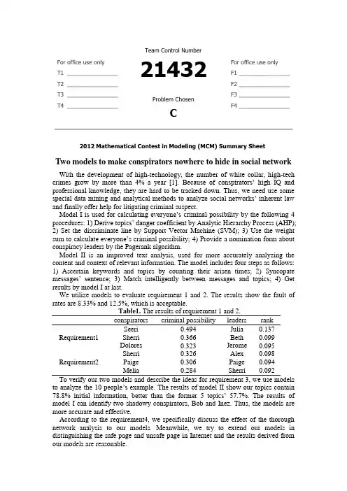
For office use onlyT1________________ T2________________ T3________________ T4________________Team Control Number21432Problem ChosenCFor office use onlyF1________________F2________________F3________________F4________________2012 Mathematical Contest in Modeling (MCM) Summary SheetTwo models to make conspirators nowhere to hide in social network With the development of high-technology, the number of white collar, high-tech crimes grow by more than 4% a year [1]. Bec ause of conspirators’ high IQ and professional knowledge, they are hard to be tracked down. Thus, we need use some special data mining and analytical methods to analyze social networks’ inherent law and finally offer help for litigating criminal suspect.M odel I is used for calculating everyone’s criminal possibility by the following 4 procedures: 1) Derive topics’ danger coefficient by Ana lytic Hierarchy Process (AHP);2) Set the discriminate line by Support Vector Machine (SVM); 3) Use the weight sum to c alculate everyone’s criminal possibility; 4) Provide a nomination form about conspiracy leaders by the Pagerank algorithm.Model II is an improved text analysis, used for more accurately analyzing the content and context of relevant information. The model includes four steps as follows: 1) Ascertain keywords and topics by counting their arisen times; 2) Syncopate me ssages’ sentence; 3) Match intelligently between messages and topics; 4) Get results by model I at last.We utilize models to evaluate requirement 1 and 2. The results show the fault of rates are 8.33% and 12.5%, which is acceptable.Table1. The results of requirement 1 and 2.conspirators criminal possibility leaders rankRequirement1Seeri 0.494 Julia 0.137 Sherri 0.366 Beth 0.099 Dolores 0.323 Jerome 0.095Requirement2 Sherri 0.326 Alex 0.098 Paige 0.306 Paige 0.094 Melia 0.284 Sherri 0.092To verify our two models and describe the ideas for requirement 3, we use models to analyze the 10 people’s example. The results of model II sho w our topics contain 78.8% initial information, better than the former 5 topics’ 57.7%. The results of model I can identify two shadowy conspirators, Bob and Inez. Thus, the models are more accurate and effective.According to the requirement4, we specifically discuss the effect of the thorough network analysis to our models. Meanwhile, we try to extend our models in distinguishing the safe page and unsafe page in Internet and the results derived from our models are reasonable.Two models to make conspirators nowhere to hideTeam #13373February 14th ,2012ContentIntroduction (3)The Description of the Problem (3)Analysis (3)What is the goal of the Modeling effort? (4)Flow chart (4)Assumptions (5)Terms, Definitions and Symbols (5)Model I (6)Overview (6)Model Built (6)Solution and Result (9)Analysis of the Result (10)Model II (11)Overview (11)Model Built (11)Result and Analysis (12)Conclusions (13)Technical summary (13)Strengths and Weaknesses (13)Extension (14)Reference (14)Appendix (16)IntroductionWith the development of our society, more and more high-tech conspiracy crimes and white-collar crimes take place in business and government professionals. Unlike simple violent crime, it is a kind of bran-new crime style, would gradually create big fraud schemes to hurt others’ benefit and destroy business companies.In order to track down the culprits and stop scams before they start, we must make full use of effective simulation model and methodology to search their criminal information. We create a Criminal Priority Model (CPM) to evaluate every suspect’s criminal possibility by analyzing text message and get a priority line which is helpful to ICM’s investigation.In addition, using semantic network analysis to search is one of the most effective ways nowadays; it will also be helpful we obtain and analysis semantic information by automatically extract networks using co-occurrence, grammatical analysis, and sentiment analysis. [1]During searching useful information and data, we develop a whole model about how to effective search and analysis data in network. In fact, not only did the coalescent of text analysis and disaggregated model make a contribution on tracking down culprits, but also provide an effective way for analyzing other subjects. For example, we can utilize our models to do the classification of pages.In fact, the conditions of pages’classification are similar to criminological analysis. First, according to the unsafe page we use the network crawler and Hyperlink to find the pages’ content and the connection between each pages. Second, extract the messages and the relationships between pages by Model II. Third, according to the available information, we can obtain the pages’priority list about security and the discriminate line separating safe pages and the unsafe pages by Model I. Finally we use the pages’ relationships to adjust the result.The Description of the ProblemAnalysisAfter reading the whole ICM problem, we make a depth analysis about the conspiracy and related information. In fact, the goal of ICM leads us to research how to take advantage of the thorough network, semantic, and text analyses of the message contents to work out personal criminal possibility.At first, we must develop a simulation model to analysis the current case’s data, and visualize the discriminate line of separating conspirator and non-conspirator.Then, by increasing text analyses to research the possible useful information from “Topic.xls”, we can optimize our model and develop an integral process of automatically extract and operate database.At last, use a new subject and database to verify our improved model.What is the goal of the Modeling effort?●Making a priority list for crime to present the most likely conspirators●Put forward some criteria to discriminate conspirator and non-conspirator, createa discriminate line.●Nominate the possible conspiracy leaders●Improve the model’s accuracy and the credit of ICM●Study the principle and steps of semantic network analysis●Describe how the semantic network analysis could empower our model.Flow chartFigure 1Assumptions●The messages have no serious error.●These messages and text can present what they truly mean.●Ignore special people, such as spy.●This information provided by ICM is reasonable and reliable.Terms, Definitions and SymbolsTable 2. Model parametersParameter MeaningThe rate of sending message to conspirators to total sending messageThe rate of receiving message to conspirators to total receiving messageThe dangerous possibility of one’s total messagesThe rate of messages with known non-conformist to total messagesDanger coefficient of topicsThe number of one’s sending messagesThe number of one’s receiving messagesThe number of one’s sending messages from criminalThe number of one’s receiving messages from criminalThe number of one’s sending messages from non-conspiratorThe number of one’s receiving messages from non-conspiratorDanger coefficient of peopleModel IOverviewModel I is used for calculating and analyzing everyone’s criminal possibility. In fact, the criminal possibility is the most important parameter to build a priority list and a discriminate line. The model I is made up of the following 4 procedures: (1) Derive topics’danger coefficient by Analytic Hierarchy Process (AHP); (2) Set the discriminate line by Support Vector Machine (SVM); (3) Use the weight sum to calculate everyone’s criminal possibility; (4) Provide a nomination form about conspiracy leaders by the Pagerank algorithm.Model BuiltStep.1PretreatmentIn order to decide the priority list and discriminate line, we must sufficiently study the data and factors in the ICM.For the first, we focus on the estimation about the phenomena of repeated names. In the name.xls, there are three pair phenomena of repeated names. Node#7 and node#37 both call Elsie, node#16 and node#34 both call Jerome, node#4 and node#32 both calls Gretchen. Thus, before develop simulation models; we must evaluate who are the real Elsie, Jerome and Gretchen.To decide which one accord with what information the problem submitsFirst we study the data in message.xls ，determine to analysis the number of messages of Elsie, Jerome and Gretchen. Table1 presents the correlation measure of their messages with criminal topic.Figure2By studying these data and figures, we can calculate the rate of messages about criminal topic to total messages; node#7 is 0.45455, while node#37 is 0.27273. Furthermore node#7 is higher than node#37 in the number of messages.Thus, we evaluate that node #7 is more likely Elsie what the ICM points out.In like manner, we think node#34, node#32 are those senior managers the ICM points out. In the following model and deduction, we assume node#7 is Elsie, node#34 is Jerome and node #32 is Gretchen.Step.2Derive topics’ danger coefficient by Analytic Hierarchy ProcessUse analytic hierarchy process to calculate the danger every topic’s coefficient. During the research, we decide use four factors’ effects to evaluate ：● Aim ：Evaluate the danger coefficient of every topic.[2]● Standard ：The correlation with dangerous keywordsThe importance of the topic itselfThe relationship of the topic and known conspiratorsThe relationship of the topic and known non-conspirators● Scheme ： The topics (1,2,3……15)Figure3According to previous research, we decide the weight of The Standard to Aim ：These weights can be evaluated by paired comparison algorithm, and build a matrix about each part.For example, build a matrix about Standard and Aim, the equation is followingij j i a C C ⇒:ijji ij n n ij a a a a A 1,0)(=>=⨯ The other matrix can be evaluated by the similar ways. At last, we make a consistency check to matrix A and find it is reasonable.The result shows in the table, and we can use the data to continue the next model. Step.3 Use the weight sum to calculate everyone ’s criminal possibilityWe will start to study every one’s danger coefficient by using four factors,, and .[3]100-第一份工作开始时间）（第一份工作结束时间第一份工作持续时间=The first factor means calculate the rate of someone’s sending criminal messages to total sending messages.The second factors means calculate the rate of someone’s receivingcriminal messages to total receiving messages.=The third factormeans calculate the dangerous possibility of someone’stotal messages.The four factorthe rate of someone’s messages with non-conspirators tototal messages.At last, we use an equation to calculate every one’s criticality, namely thepossibility of someone attending crime. ( Shows every factors’weighing parameter)After calculating these equations abov e, we derive everyone’s criminal possibilityand a priority list. (See appendix for complete table about who are the most likely conspirators) We instead use a cratering technique first described by Rossmo [1999]. The two-dimensional crime points xi are mapped to their radius from the anchor point ai, that is, we have f : xi → ri, where f(xi) = j i i a a (a shifted modulus). The set ri isthen used to generate a crater around the anchor point.There are two dominatingStep.4 Provide a nomination form about conspiracy leaders by the Pagerankalgorithm.At last, we will find out the possible important leaders by pagerank model, and combined with priority list to build a prior conspiracy leaders list.[4]The essential idea from Page Rank is that if node u has a link to node v, then the author of u is an implicitly conferring some importance to node v. Meanwhile it means node v has a important chance. Thus, using B (u) to show the aggregation of links to node u, and using F (u) to show the aggregation of received links of node u, The C is Normalization factor. In each iteration, propagate the ranks as follows: The next equation shows page rank of node u:Using the results of Page Rank and priority list, we can know those possiblecriminal conspiracy leaders.Solution and ResultRequirement 1:According to Model I above, we calculate these data offered by requirement 1 and build two lists. The following shows the result of requirement 1.By running model I step2, we derive danger coefficient of topics, the known conspiracy topic 7, 11 and 13 are high danger coefficient (see appendix Table4. for complete information).After running model step3, we get a list of every one’s criticality .By comparing these criticality, we can build a priority list about criminal suspects. In fact, we find out criminal suspects are comparatively centralized, who are highly different from those known non-conspirators. This illuminates our model is relative reasonable. Thus we decide use SVM to get the discriminate line, namely to separate criminal suspects and possible non-conspirators (see appendix Table5. for complete information). Finally, we utilize Page rank to calculate criminal suspects’ Rank and status, table4 shows the result. Thus, we nominate 5 most likely criminal leaders according the results of table4.They are Julia, Beth, Jerome, Stephanie and Neal.According to the requirement of problem1, we underscore the situations of three senior managers Jerome, Delores and Gretchen. Because the SVM model makes a depth analysis about conspirators, Jerome is chosen as important conspirator, Delores and Gretchen both has high danger coefficient. We think Jerome could be a conspirator, while Delores and Gretchen are regarded as important criminal suspects. Using the software Ucinet, we derive a social network of criminal suspects.The blue nodes represent non-conspirators. The red nodes represent conspirators. The yellow nodes represent conspiracy leaders.Figure 4Requirement 2:Using the similar model above, we can continue analyzing the results though theconditions change.We derive three new tables (4, 5 and 6): danger coefficient of topics, every one’s criticality and the probability of nominated. At last, we get a new priority list (table6) and 5 most likely criminal leaders: Alex, Sherri, Yao, Elsie and Jerome.We sincerely wish that our analysis can be helpful to ICM’s investigation. We figure out a new figure, which shows the social network of criminal suspects for requirement 2.Figure 5Analysis of the Result1)AnalysisIn the requirement 1, we find out 24 possible criminal suspects. All of 7 known conspirators are in the 24 suspects and their danger coefficients are also pretty high. However, there are 2 known non-conspirators are in these suspects.Thus, the rate of making mistakes is 8.33%. In all, we still have enough reasons to think the model is reasonable.In addition, we find 5 suspects who are likely conspirators by Support Vector Machine (SVM).In the requirement 2, we also choose 24 the most likely conspirators after run our CPM. All of 8 known conspirators are also in the 24 suspects and their danger coefficients are pretty high. Because 3 known non-conspirators are in these suspects, the rate of making mistakes is 12.5%, which is higher to the result of requirement 1.2)ComparisonTo research the effect of changing the number of criminal topics and conspirators to results, we decide to do an additional research about their effect.We separate the change of topics and crimes’numbers, analysis result’s changes of only one factor:In order to analyze the change between requirement 1 and 2, we choose those people whose rank has a big change over 30.Reference: the node.1st result: the part of the requirement1’s priority list.2nd result: the part of the requirement2’s priority list.3rd result: the priority’s changes of requirement 1 and 2.After investigate these people, we find out the topics about them isn’t close connected with node#0. Thus, the change of node#0 does not make a great effect on their change.However, there are more than a half of people who talk about topic1. According to the analysis, we find the topic1 has a great effect on their change. The topic1 is more important to node#0.Thus; we can do an assumption that the decision of topics has bigger effect on the decision of the personal identity and decide to do a research in the following content.Model IIOverviewAccording to requirement3, we will take the text analysis into account to enhance our model. In the paper, text analysis is presented as a paradigm for syntactic-semantic analysis of natural language. The main characteristics of this approach are: the vectors of messages about keywords, semanteme and question formation. In like manner, we need get three vectors of topics. Then, we utilize similarity to separate every message to corresponding topics. Finally, we evaluate these effects of text analysis by model I.Model BuiltStep.1PretreatmentIn this step, we need conclude relatively accurate topics by keywords in messages. Not only builds a database about topics, but also builds a small database for adjusting the topic classification of messages. The small database for adjusting is used for studying possible interpersonal relation between criminal suspects, i. e. Bob always use positive and supportive words to comment topics and things about Jerry, and then we think Bob’s messages are closely connected with topics about Jerry. [5] At first, we need to count up how many keywords in the whole messages.Text analysis is word-oriented, i.e., the word plays the central role in language understanding. So we avoid stipulating a grammar in the traditional sense and focus on the concept of word. During the analysis of all words in messages, we ignore punctuation, some simple word such as “is” and “the”, and extract relative importantwords.Then, a statistics will be completed about how many times every important word occurs. We will make a priority list and choose the top part of these words.Finally, according to some messages, we will turn these keywords into relatively complete topics.Step.2Syncopate sentenceWe will make a depth research to every sentence in messages by running program In the beginning, we can utilize the same way in step1 to syncopate sentence, deriving every message’s keywords. We decide create a vector about keywords: = () (m is the number keywords in everymessage)For improving the accuracy and relativity of our keywords, we decide to build a vector that shows every keyword’s synonyms, antonym.= () (1<k<m, p is the number of correlative words)According to primary analysis, we can find some important interpersonal relations between criminal suspects, i.e. Bob is closely connected with Jerry, then we can build a vector about interpersonal relation.= () (n is the number of relationships in one sentence )Step.3Intelligent matchingIn order to improve the accuracy of our disaggregated model, we use three vectors to do intelligent matching.Every message has three vectors:. Similarly, every topic alsohas three vectors.At last, we can do an intelligent matching to classify. [6]Step.4Using CPMAfter deriving new the classification of messages, we will make full use of new topics to calculate every one’s criticality.Result and AnalysisAfter calculating the 10 people example, we derive new topics. By verifying the topics’ contained initial information, we can evaluate the effect of models.The results of model II show our topics contain 78.8% initial information, better than former 5 topics’ 57.7%.T hus, new topics contain more initial information. Meanwhile, we build a database about interpersonal relation, and using it to optimize the results of everyone’s criminal possibility.Table 3#node primary new #node primary new1 0 0.065 6 0.342 0.2652 0.342 0.693 7 0.891 0.9123 0.713 0.562 8 0.423 0.354 1 1 9 0.334 0.7235 0.823 0.853 10 0.125 0.15 The results of model I can identify the two shadowy conspirators, Bob and Inez. In the table, the rate of fault is becoming smaller.According to Table11, we can derive some information:1.Analysis the danger coefficient of two people, Bob and Inez. Bob is theperson who self-admitted his involvement in a plan bargain for a reducedsentence. His data changes from 0.342 to 0.693. And Inez is the person whogot off, his data changes from 0.334 to 0.723. The models can identify thetwo shadowy people.2.Carol, the person who was later dropped his data changes from 0.713 to0.562. Although it still has a relatively high danger coefficient, the resultsare enhancing by our models.3.The distance between high degree people and low degree become bigger, itpresents the models would more distinctly identify conspirators andnon-conspirators.Thus, the models are more accurate and effective.ConclusionsTechnical summaryWe bring out a whole model about how to extract and analysis plentiful network information, and finally solve the classification problems. Four steps are used to make the classification problem easier.1)According known conspirators and correlative information, use resemblingnetwork crawler to extract what we may need information and messages.[7]2)Using the second model to analysis and classify these messages and text, getimportant topics.3)Using the first model to calculate everyone’s criminal possibility.4)Using an interpersonal relation database derived by step2 to optimize theresults. [8]Strengths and WeaknessesStrengths:1）We analyze the danger coefficient of topics and people by using different characteristics to describe them. Its results have a margin of error of 10percentage points. That the Models work well.2）In the semantic analysis, in addition to obtain topics from messages in social network, we also extract the relationships of people and adjust the final resultimprove the model.3）We use 4 characteristics to describe people’s danger coefficient. SVM has a great advantage in classification by small characteristics. Using SVM to classify the unknown people and its result is good.Weakness：1）For the special people, such as spy and criminal researcher, the model works not so well.2）We can determine some criminals by topics; at the same time we can also use the new criminals to adjust the topics. The two react upon each other. We canexpect to cycle through several times until the topics and criminals are stable.However we only finish the first cycle.3）For the semantic analysis model we have established, we just test and verify in the example (social network of 10 people). In the condition of large social network, the computational complexity will become greater, so the classify result is still further to be surveyed.ExtensionAccording to our analysis, not only can our model be applied to analyze criminal gangs, but also applied to similar network models, such as cells in a biological network, safe pages in Internet and so on. For the pages’ classification in Internet, our model would make a contribution. In the following, we will talk about how to utilize [9] Our model in pages’ classification.First, according to the unsafe page we use the network crawler and Hyperlink to find the pages’content and the connection between each page. Second, extract the messages and the relationships between pages by Model II. Third, according to the available information, we can obtain the pages’priority list about security and the discriminate line separating safe pages and the unsafe pages by Model I. Finally we use the pages’ relationships to adjust the result.Reference1. http://books.google.pl/books?id=CURaAAAAYAAJ&hl=zh-CN2012.2. AHP./wiki/%E5%B1%82%E6%AC%A1%E5%88%86%E6%9E%90%E6%B 3%95.3. Schaller, J. and J.M.S. Valente, Minimizing the weighted sum of squared tardiness on a singlemachine. Computers & Operations Research, 2012. 39(5): p. 919-928.4. Frahm, K.M., B. Georgeot, and D.L. Shepelyansky, Universal emergence of PageRank.Journal of Physics a-Mathematical and Theoretical, 2011. 44(46).5. Park, S.-B., J.-G. Jung, and D. Lee, Semantic Social Network Analysis for HierarchicalStructured Multimedia Browsing. Information-an International Interdisciplinary Journal, 2011.14(11): p. 3843-3856.6. Yi, J., S. Tang, and H. Li, Data Recovery Based on Intelligent Pattern Matching.ChinaCommunications, 2010. 7(6): p. 107-111.7. Nath, R. and S. Bal, A Novel Mobile Crawler System Based on Filtering off Non-ModifiedPages for Reducing Load on the Network.International Arab Journal of Information Technology, 2011. 8(3): p. 272-279.8. Xiong, F., Y. Liu, and Y. Li, Research on Focused Crawler Based upon Network Topology.Journal of Internet Technology, 2008. 9(5): p. 377-380.9. Huang, D., et al., MyBioNet: interactively visualize, edit and merge biological networks on theWeb. Bioinformatics, 2011. 27(23): p. 3321-3322.AppendixTable 4requirement 1topic danger topic danger topic danger topic danger7 1.65 4 0.78 5 0.47 8 0.1713 1.61 10 0.77 15 0.46 14 0.1711 1.60 12 0.47 9 0.19 6 0.141 0.812 0.473 0.18requirement 2topic danger topic danger topic danger topic danger1 0.402 0.26 15 0.15 14 0.117 0.37 9 0.23 8 0.15 3 0.0913 0.37 10 0.21 5 0.14 6 0.0611 0.30 12 0.18 4 0.12Table 5requirement 1#node danger #node danger #node danger #node danger 21 0.74 22 0.19 0 0.13 23 0.03 67 0.69 4 0.19 40 0.13 72 0.03 54 0.61 33 0.19 36 0.13 62 0.03 81 0.49 47 0.19 11 0.12 51 0.02 7 0.47 41 0.19 69 0.12 57 0.02 3 0.37 28 0.18 29 0.12 64 0.02 49 0.36 16 0.18 12 0.11 71 0.02 43 0.36 31 0.17 25 0.11 74 0.01 10 0.32 37 0.17 82 0.11 58 0.01 18 0.29 27 0.16 60 0.10 59 0.01 34 0.29 45 0.16 42 0.10 70 0.00 48 0.28 50 0.16 65 0.09 53 0.00 20 0.27 24 0.16 9 0.09 76 0.00 15 0.27 44 0.16 5 0.09 61 0.00 17 0.26 38 0.16 66 0.09 75 -0.01 2 0.23 13 0.16 26 0.08 77 -0.01 32 0.23 35 0.15 39 0.06 55 -0.02 30 0.20 1 0.15 80 0.04 68 -0.02 73 0.20 46 0.15 78 0.04 52 -0.0319 0.20 8 0.14 56 0.03 63 -0.03 14 0.19 6 0.14 79 0.03requirement 2#node danger #node danger #node danger #node danger 0 0.39881137 75 0.1757106 47 0.1090439 11 0.0692506 21 0.447777778 52 0.1749354 71 0.1089147 4 0.0682171 67 0.399047158 38 0.1738223 82 0.1088594 42 0.0483204 54 0.353754153 10 0.1656977 14 0.1079734 65 0.046124 81 0.325736434 19 0.1559173 27 0.1060724 60 0.0459948 2 0.306054289 40 0.1547065 23 0.105814 39 0.0286822 18 0.303178295 30 0.1517626 5 0.1039406 62 0.0245478 66 0.28372093 80 0.145155 8 0.10228 78 0.0162791 7 0.279870801 24 0.1447674 73 0.1 56 0.0160207 63 0.261886305 70 0.1425711 50 0.0981395 64 0.0118863 68 0.248514212 29 0.1425562 26 0.097213 72 0.011369548 0.239668277 45 0.1374667 1 0.0952381 79 0.009302349 0.238076781 37 0.1367959 69 0.0917313 51 0.0056848 34 0.232614868 17 0.1303064 33 0.0906977 57 0.0056848 3 0.225507567 6 0.1236221 31 0.0905131 74 0.0054264 35 0.222435188 22 0.1226934 36 0.0875452 76 0.005168 77 0.214470284 13 0.1222868 41 0.0822997 53 0.0028424 20 0.213718162 44 0.115007 46 0.0749354 58 0.0015504 43 0.204328165 12 0.1121447 28 0.0748708 59 0.0015504 32 0.193311469 15 0.1121447 16 0.074234 61 0.0007752 55 0.182687339 9 0.1117571 25 0.0701292Table 6requirement 1#node leader #node leader #node leader #node leader 15 0.1368 49 0.0481 7 0.0373 19 0.0089 14 0.0988 4 0.0423 21 0.0357 32 0.0073 34 0.0951 10 0.0422 18 0.029 22 0.0059 30 0.0828 67 0.0421 48 0.0236 81 0.0053 17 0.0824 54 0.0377 20 0.0232 73 043 0.0596 3 0.0377 2 0.0181 33 0requirement 2#node leader #node leader #node leader #node leader 21 0.0981309 7 0.0714406 54 0.0526831 43 0.01401872 0.0942899 34 0.0707246 32 0.0464614 81 0.00977763 0.0916127 0 0.0706746 18 0.041114248 0.0855984 20 0.0658119 68 0.028532867 0.0782211 49 0.0561665 35 0.024741。