ANSYS热应力分析实例教学教材

05
热分析优化设计
优化设计的基本概念
01
优化设计是一种通过数学模型和计算机技术，寻找满足特定条 件下的最优设计方案的方法。
02
优化设计的基本概念包括目标函数、设计变量、约束条件和求
解算法等。
热分析优化设计是针对热学问题，通过优化设计来提高产品的
03
热性能和降低能耗。
ANSYS优化设计的步骤
定义设计变量
网格质量检查
对生成的网格进行检查， 确保网格质量良好，没有 出现奇异点或扭曲。
边界条件的设置
确定边界条件
根据分析对象的实际情况，确定合适的边界条件，如温度、热流 率等。
设置边界条件
在ANSYS软件中，将确定的边界条件应用到几何模型上。
验证边界条件
对设置的边界条件进行验证，确保其合理性和准确性。
04
傅里叶定律
热量传递与温度梯度成正比，即热流密度与温度梯度 成正比。
牛顿冷却定律
物体表面与周围介质之间的温差与热流密度成正比。
热力学第一定律
能量守恒定律，表示系统能量的增加等于传入系统的 热量与系统对外界所做的功之和。
热分析的三种基本类型
稳态热分析
系统达到热平衡状态时的温度分布。
瞬态热分析
系统随时间变化的温度分布。
网格划分问题
网格划分不均匀
在某些区域，网格可能过于密集，而 在其他区域则可能过于稀疏，这可能 导致求解精度下降或求解失败。
网格自适应调整问题
在某些情况下，ANSYS可能无法正确 地自适应调整网格，导致求解结果不 准确。
网格划分问题
手动调整网格
手动调整网格密度，确保在关键区域有足够的网格密度。
使用更高级的网格划分工具

实体单元
网格划分
FEA 模型
Ansys 应力分析
应力分析 - 前处理
...网格划分
• 网格划分的三个步骤:
• 定义单元属性 • 指定网格控制 • 生成网格
• 单元属性 是网格划分前必须建立的有限单元模型
属性。它们包括:
• 单元类型 • 实常数 • 材料性质
Ansys 应力分析
应力分析 - 前处理
应力分析 - 前处理
B. 几何模型
• 典型的实体模型是由体、面、线和关键点组成的 。
• 体 由面围成，用来描述实体物体。 • 面 由线围成，用来描述物体的表面或者块、壳等。 • 线 由关键点组成，用来描述物体的边。 • 关键点 是三维空间的位置， 用来描述物体的顶点。
体
面
线和关键点
Ansys 应力分析
• 在弹出的对话框中，选择 No defeaturing * (缺省值) ，按下 OK (默
认其他选项)。 • 在第二个对话框中选择想要的文件并
点击OK.
• 或使用 IGESIN 命令:
• /aux15 • ioptn,iges,nodefeat • igesin, • finish
* 关于 No Defeaturing 及 Defeaturing 方法及其他选项将在后面论述
• 求解
• 施加载荷 • 求解
• 后处理
• 结果评价 • 检查结果的正确性
Ansys 应力分析
前处理 求解 后处理
应力分析
...应力分析步骤
• 注意！ANSYS 的主菜单也是按照前处理、求解、 后处理来组织的
Ansys 应力分析
应力分析
...应力分析步骤
• 前处理器 (在ANSYS中称为 PREP7) 提供了对程序 的主要输入

汽车发动机热分析
总结词
汽车发动机热分析用于研究发动机工作过程中的热量传递和热应力分布，以提高发动机 效率和可靠性。
详细描述
发动机是汽车的核心部件，其工作过程中会产生大量的热量。通过热分析，工程师可以 了解发动机内部的温度分布和热应力状况，优化发动机设计，提高其燃油效率和耐久性
。
建筑物的温度分布分析
热分析的基本原理
热分析是研究温度场分布、变化 和传递规律的科学，其基本原理 包括能量守恒、热传导、对流和 辐射等。
热分析的应用领域
热分析广泛应用于能源、动力、 化工、机械、电子等众多领域， 涉及传热、燃烧、材料热物性、 电子器件散热等方面。
热分析的常用软件
ANSYS是国际上最流行的热分析 软件之一，具有强大的建模、网 格划分、加载、求解和后处理功 能，广泛应用于工程实际和科学 研究。
模拟系统在稳定状态下温度分布和热流密 度的计算方法
总结词
适用于研究系统在稳定状态下的热性能和 热量传递机制。
详细描述
稳态热分析用于计算系统在稳定状态下温 度分布和热流密度，不考虑时间因素，只 考虑热平衡状态。
详细描述
在稳态热分析中，系统的温度分布和热流 密度不随时间变化，因此可以忽略时间积 分效应，简化计算过程。
施加边界条件和载荷
根据实际情况，为模型的边界施加固 定温度、热流等边界条件，以及热载 荷。
求解和结果查看
选择求解器
根据模型的大小和复杂程度，选择合适的求解器进行求解。
结果后处理与查看
查看温度分布、热流分布等结果，并进行必要的后处理，如云图显示、数据导 出等。
03
热分析的常用方法
稳态热分析
总结词
COMSOL Multiphysics

第四讲 热分析上机指导书CAD/CAM 实验室，USTC实验要求：1、通过对冷却栅管的热分析练习，熟悉用ANSYS 进行稳态热分析的基本过程，熟悉用直接耦合法、间接耦合法进行热应力分析的基本过程。

2、通过对铜块和铁块的水冷分析，熟悉用ANSYS 进行瞬态热分析的基本过程。

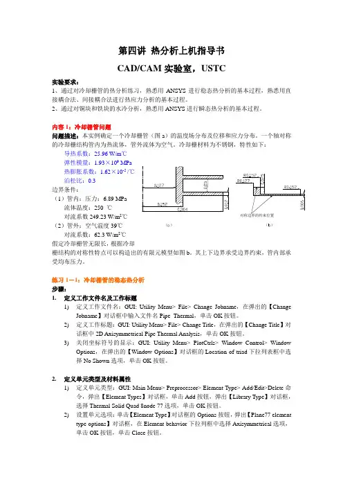
内容1：冷却栅管问题问题描述：本实例确定一个冷却栅管（图a ）的温度场分布及位移和应力分布。

一个轴对称的冷却栅结构管内为热流体，管外流体为空气。

冷却栅材料为不锈钢，特性如下： 导热系数：25.96 W/m ℃弹性模量：1.93×109 MPa热膨胀系数：1.62×10-5 /℃泊松比：0.3边界条件：（1）管内：压力：6.89 MPa流体温度：250 ℃对流系数249.23 W/m 2℃（2）管外：空气温度39℃对流系数：62.3 W/m 2℃假定冷却栅管无限长，根据冷却栅结构的对称性特点可以构造出的有限元模型如图b 。

其上下边界承受边界约束，管内部承受均布压力。

练习1－1：冷却栅管的稳态热分析步骤：1. 定义工作文件名及工作标题1) 定义工作文件名：GUI: Utility Menu> File> Change Jobname ，在弹出的【Change Jobname 】对话框中输入文件名Pipe_Thermal ，单击OK 按钮。

2) 定义工作标题：GUI: Utility Menu> File> Change Title ，在弹出的【Change Title 】对话框中2D Axisymmetrical Pipe Thermal Analysis ，单击OK 按钮。

3) 关闭坐标符号的显示：GUI: Utility Menu> PlotCtrls> Window Control> Window Options ，在弹出的【Window Options 】对话框的Location of triad 下拉列表框中选择No Shown 选项，单击OK 按钮。

PLANE75 四节点轴对称单元
PLANE78 八节点轴对称单元
三维实体SOLID87 六节点四面体单元
SOLID70
八节点六面体单元
SOLID90
二十节点六面体单元
壳
SHELL57 四节点
点
MASS71
有关单元的详细解释，请参阅《ANSYS Element Reference
Guide》
3 热分析基本过程
[C]{ }+[K]{T}={Q}
式中: [K]为传导矩阵，包含导热系数、对流 系数及辐射率和形状系数；
[C]为比热矩阵,考虑系统内能的增加;
{T}为节点温度向量；
{ }为温度对时间的导数;
{Q}为节点热流率向量，包含热生成。
6、线性与非线性
如果有下列情况产生，则为非线性热分析：
①、材料热性能随温度变化，如K(T),C(T)等 ；
射率和形状系数；
{T}为节点温度向量；
{Q}为节点热流率向量，包含热生成；
ANSYS利用模型几何参数、材料热性能参数以及
所施加的边界条件，生成[K] 、 {T}以及{Q} 。
6、瞬态传热
瞬态传热过程是指一个系统的加热或冷却过程 。在这个过程中系统的温度、热流率、热边界 条件以及系统内能随时间都有明显变化。根据 能量守恒原理，瞬态热平衡可以表达为（以矩 阵形式表示）：
Command Family: F GUI：Main Menu>Solution>-Loads-Apply>-Thermal-
Heat Flux
e、生热率
生热率作为体载施加于单元上，可以模拟化 学反应生热或电流生热。它的单位是单位 体积的热流率。
Command Family: BF GUI：Main Menu>Solution>-Loads-Apply>-

(13) 定义材料参数 Main Menu → Preprocessor → Material Props → Material Models → Material Models Available: Structural（双击打开子菜单） → Linear（双击） → Elastic （双击）→ Isotropic（双击） → EX： 2.0e5 (弹性模量) ，PRXY：0.3 (泊松比)→ OK →转到Material Models Available: Thermal Expansion（双击） →Secant Coefficient （双击）→ Isotropic（双击） →ALPX：1.2E-5(平均线膨胀系数) → OK →关闭材料 定义菜单（点击菜单的右上角X）
(3) 设置计算类型 Main Menu: Preferences… → select Thermal, steady → OK
(4) 选择单元类型 Main Menu: Preprocessor → Element Type → Add/Edit/Delete → Add → Thermal Solid，
【ANSYS 应用实例 2.1】 焊接接头稳态传热过程的数值模拟
如图 2-1 所示，圆形的冷凝管通过法兰接头进行对接。接头的制作方法如下：先把法兰 移动到圆管接头位置，然后沿圆周焊接两道次，把法兰连接到圆管上。用螺栓把两个法兰接 头拉紧，法兰之间压上一块垫片。圆管内的液体温度为 0℃，蒸汽冷凝在圆管的外表面上， 蒸汽温度为 100℃。圆管内表面换热系数为 5000W/m2K，外表面换热系数为 20000 W/m2K。
UNIT2-2
TH-FEA(应用实例-UNIT2)
清华大学 曾攀
(6) 生成几何模型 Main Menu: Preprocessor → Modeling → Create → Keypoints → In Active CS → NPT

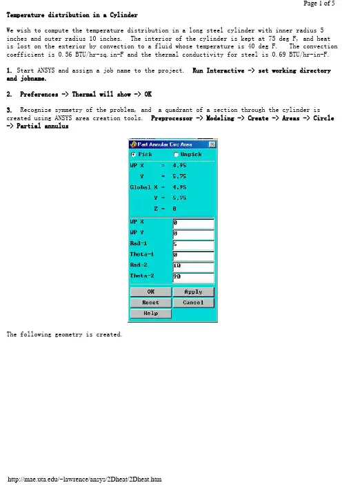
Temperature distribution in a CylinderWe wish to compute the temperature distribution in a long steel cylinder with inner radius 5 inches and outer radius 10 inches. The interior of the cylinder is kept at 75 deg F, and heatis lost on the exterior by convection to a fluid whose temperature is 40 deg F. The convection coefficient is 0.56 BTU/hr-sq.in-F and the thermal conductivity for steel is 0.69 BTU/hr-in-F.1. Start ANSYS and assign a job name to the project. Run Interactive -> set working directory and jobname.2. Preferences -> Thermal will show -> OK3. Recognize symmetry of the problem, and a quadrant of a section through the cylinder is created using ANSYS area creation tools. Preprocessor -> Modeling -> Create -> Areas -> Circle -> Partial annulusThe following geometry is created.4. Preprocessor -> Element Type -> Add/Edit/Delete -> Add -> Thermal Solid -> Solid 8 node 77 -> OK -> Close5. Preprocessor -> Material Props -> Isotropic -> Material Number 1 -> OKEX = 3.E7 (psi)DENS = 7.36E-4 (lb sec^2/in^4)ALPHAX = 6.5E-6PRXY = 0.3KXX = 0.69 (BTU/hr-in-F)6. Mesh the area and refine using methods discussed in previous examples.7. Preprocessor -> Loads -> Apply -> Temperatures -> NodesSelect the nodes on the interior and set the temperature to 75.8. Preprocessor -> Loads -> Apply -> Convection -> LinesSelect the lines defining the outer surface and set the convection coefficient to 0.56 and the fluid temp to 40.9. Preprocessor -> Loads -> Apply -> Heat Flux -> LinesTo account for symmetry, select the vertical and horizontal lines of symmetry and set the heat flux to zero.10. Solution -> Solve current LS11. General Postprocessor -> Plot Results -> Nodal Solution -> TemperaturesThe temperature on the interior is 75 F and on the outside wall it is found to be 45. These results can be checked using results from heat transfer theory.BackThermal Stress of a Cylinder using Axisymmetric ElementsA steel cylinder with inner radius 5 inches and outer radius 10 inches is 40 inches long and has spherical end caps. The interior of the cylinder is kept at 75 deg F, and heat is lost on the exterior by convection to a fluid whose temperature is 40 deg F. The convection coefficient is 0.56 BTU/hr-sq.in-F. Calculate the stresses in the cylinder caused by the temperature distribution.The problem is solved in two steps. First, the geometry is created, the preference set to'thermal', and the heat transfer problem is modeled and solved. The results of the heat transfer analysis are saved in a file 'jobname.RTH' (Results THermal analysis) when you issue a save jobname.db command.Next the heat transfer boundary conditions and loads are removed from the mesh, the preference is changed to 'structural', the element type is changed from 'thermal' to 'structural', and the temperatures saved in 'jobname.RTH' are recalled and applied as loads.1. Start ANSYS and assign a job name to the project. Run Interactive -> set working directory and jobname.2. Preferences -> Thermal will show -> OK3. A quadrant of a section through the cylinder is created using ANSYS area creation tools.4. Preprocessor -> Element Type -> Add/Edit/Delete -> Add -> Solid 8 node 77 -> OK ->Options -> K3 Axisymmetric -> OK5. Preprocessor -> Material Props -> Isotropic -> Material Number 1 -> OKEX = 3.E7 (psi)DENS = 7.36E-4 (lb sec^2/in^4)ALPHAX = 6.5E-6PRXY = 0.3KXX = 0.69 (BTU/hr-in-F)6. Mesh the area using methods discussed in previous examples.7. Preprocessor -> Loads -> Apply -> Temperatures -> NodesSelect the nodes on the interior and set the temperature to 75.8. Preprocessor -> Loads -> Apply -> Convection -> LinesSelect the lines defining the outer surface and set the coefficient to 0.56 and the fluid temp to 40.9. Preprocessor -> Loads -> Apply -> Heat Flux -> LinesSelect the vertical and horizontal lines of symmetry and set the heat flux to zero.10. Solution -> Solve current LS11. General Postprocessor -> Plot Results -> Nodal Solution -> TemperatureThe temperature on the interior is 75 F and on the outside wall it is found to be 43.12. File -> Save Jobname.db13. Preprocessor -> Loads -> Delete -> Delete All -> Delete All Opts.14. Preferences -> Structural will show, Thermal will NOT show.15. Preprocessor -> Element Type -> Switch Element Type -> OK (This changes the element to structural)16. Preprocessor -> Loads -> Apply -> Displacements -> Nodes(Fix nodes on vertical and horizontal lines of symmetry from crossing the lines of symmetry.)17. Preprocessor -> Loads -> Apply -> Temperature -> From Thermal AnalysisSelect Jobname.RTH (If it isn't present, look for the default 'file.RTH' in the root directory)18. Solution -> Solve Current LS19. General Postprocessor -> Plot Results -> Element Solution - von Mises StressThe von Mises stress is seen to be a maximum in the end cap on the interior of the cylinder and would govern a yield-based design decision.Back。

文档收集于互联网，已重新整理排版.word版本可编辑.欢迎下载支持. 6-1•本章练习稳态热分析的模拟，包括：A. 几何模型B. 组件-实体接触C. 热载荷D. 求解选项E. 结果和后处理F. 作业6.1• 本节描述的应用一般都能在ANSYS DesignSpace Entra或更高版本中使用，除了ANSYS Structural• 提示：在ANSYS 热分析的培训中包含了包括热瞬态分析的高级分析K T T= Q T –在稳态分析中不考虑瞬态影响–[K] 可以是一个常量或是温度的函数–{Q}可以是一个常量或是温度的函数•上述方程基于傅里叶定律：• 固体内部的热流（Fourier’s Law）是[K]的基础；• 热通量、热流率、以及对流在{Q} 为边界条件；•对流被处理成边界条件，虽然对流换热系数可能与温度相关•在模拟时，记住这些假设对热分析是很重要的。

•热分析里所有实体类都被约束：–体、面、线•线实体的截面和轴向在D esignModeler中定义• 热分析里不可以使用点质量（Point Mass）的特性•壳体和线体假设：–壳体：没有厚度方向上的温度梯度–线体：没有厚度变化，假设在截面上是一个常量温度• 但在线实体的轴向仍有温度变化•唯一需要的材料特性是导热性（Thermal Conductivity）•Thermal Conductivity在Engineering Data 中输入•温度相关的导热性以表格形式输入若存在任何的温度相关的材料特性，就将导致非线性求解。

•对于结构分析，接触域是自动生成的，用于激活各部件间的热传导–如果部件间初始就已经接触，那么就会出现热传导。

–如果部件间初始就没有接触，那么就不会发生热传导（见下面对pinball的解释）。

–总结：–Pinball区域决定了什么时候发生接触，并且是自动定义的，同时还给了一个相对较小的值来适应模型里的小间距。

•如果接触是Bonded（绑定的）或no separation（无分离的），那么当面出现在pinball radius内时就会发生热传导（绿色实线表示）。

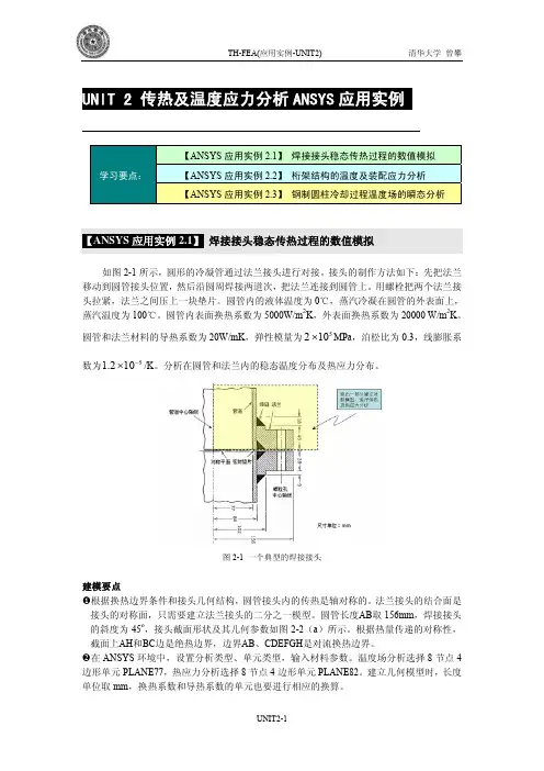
热流体在代有冷却栅的管道里流动，如图为其轴对称截面图。

管道及冷却栅的材料均为不锈钢，导热系数为1.25Btu/hr-in-oF，弹性模量为28E6lb/in2泊松比为0.3。

管内压力为1000 lb/in2，管内流体温度为450 oF，对流系数为1 Btu/hr-in2-oF,外界流体温度为70 oF，对流系数为0.25 Btu/hr-in2-oF。

求温度及应力分布。

7.3.2菜单操作过程7.3.2.1设置分析标题1、选择“Utility Menu>File>Change Title”，输入Indirect thermal-stress Analysis of a cooling fin。

2、选择“Utility Menu>File>Change Filename”，输入PIPE_FIN。

7.3.2.2进入热分析，定义热单元和热材料属性1、选择“Main Menu>Preprocessor>Element Type>Add/Edit/Delete”，选择PLANE55，设定单元选项为轴对称。

2、设定导热系数：选择“Main Menu>Preprocessor>Material Porps>Ma terial Models”，点击Thermal，Conductivity，Isotropic，输入1.25。

7.3.2.3创建模型1、创建八个关键点，选择“Main Menu>Preprocessor>Creat>Keypoints>On Active CS”，关键点的坐标如下：3、设定单元尺寸，并划分网格：“Main Menu>Preprocessor>Meshtool”，设定global size为0.125，选择AREA，Mapped，Mesh，点击Pick all。

7.3.2.4施加荷载1、选择“Utility Menu>Select>Entities>Nodes>By location>X coordinates，From Full”，输入5，点击OK，选择管内壁节点；2、在管内壁节点上施加对流边界条件：选择“MainMenu>Solution>Apply>Convection>On nodes”，点击Pick，all，输入对流换热系数1，流体环境温度450。

23
双击“Thermal Expansion、Secant Coefficient、Isotropic”。
24
输入热膨胀系数为15e-6，参考温度20。
25
施加载荷
1.施加温度载荷。 Main Menu>Preprocessor>Loads>Define Loads>Apply>Structural>Temperature>From Therm Analy
3
重点学习内容
1.间接法热应力分析步骤。 2.掌握平面应变的解决方案。 3.掌握对称结构分析方案。 4. 掌握稳态温度场计算方法。
4
更改文件名
更改文件名：Utility Menu> File> Change Jobname
5
选择单元
选择55号单元
Main Menu> Preprocessor> Element Type> Add/Edit/Delete
6
设置材料属性
1.给定材料的导热系数40W/(m·℃) 。
Main Menu> Preprocessor> Material Props> Material Models
7
建立实体模型（国际单位制）
1. 创建矩形A1：x1,y1(0,0)、x2,y2(0.01,0.07) MainMenu>Preprocessor>Modeling>Create>Areas>Rectangle>By Dimensions 2. 创建矩形A2：x1,y1(0,0.05)、x2,y2(0.08,0.07) 3.显示面的编号 Utility Menu>PlotCtrls>Numbering 4. 对面A1和A2进行overlap操作 Main Menu>Preprocessor>Modeling>Operate>Booleans> Overlap>Areas

b. 选择热分析的 结果文件，以rth为扩展名 c. 单击OK
20.4 间接耦合的分析过程(续)
9.画图核定温度 a. PlotCtrls> Symbols. b. Choose None in Boundary
Cond. Symbol c. Turn “body load symbol” to
“structural temps” d. Choose Do not replot 10.指定载荷步选项 Main Menu: Solution 在每个对话框中输入对应值 11.开始求解 Main Menu: Solution
3.求解并查看热分析结果和结构分 析结果
热分析
结构分析
合并的
jobname.rst
20.6 间接耦合和直接耦合的比较
❖ 间接耦合 ✓ 对不是高度非线性的耦合
情况, 间接方法更有效， 更灵活，因为可以相互独 立地执行两种分析 ✓ 在间接热-应力分析中， 例如，在非线性瞬态热分 析之后可以紧接着进行线 性静力分析。然后可以把 热分析中任意荷载步或时 间点的节点温度作为应力 分析的载荷
3.删除热载荷，并将分析从热分析转换到结构分析 Main Menu: Preferences a.选择结构分析。 b.单击OK。 注意：如果在开始分析时没有明确指定热分析，则
不需要转换分析类型。
20.4 间接耦合的分析过程(续)
4.将单元类型从热分析转换到结构分析 Main Menu: Preprocessor > Element Type > Switch
20.4 间接耦合的分析过程(续)
8.施加结构载荷并包括温度作为加载的一部分
Main Menu: Solution > -Load- Apply > Structure- Temperature > From Therm Analy

热分析ansys教程ppt课件
19.3 热分析的符号与单位
项目 长度 时间 质量 温度 力 能量(热量) 功率(热流率) 热流密度 生热速率 导热系数 对流系数 密度 比热 焓
国际单位
m s Kg ℃
N J W W/m2 W/m3 W/m-℃ W/m2-℃ Kg/m3 J/Kg-℃ J/m3
英制单位 ft[英尺]
19.11.3 建模
①确定jobname、title、unit； ②进入PREP7前处理，定义单元类型，设定单元
选项； ③定义单元实常数； ④定义材料热性能参数，对于稳态传热，一般只
需定义导热系数，它可以是恒定的，也可以随 温度变化； ⑤创建几何模型并划分网格。
19.11.3.1 几何尺寸(模型)
Command Family: D GUI：Main Menu>Solution>-Loads-Apply>-Thermal-
Temperature
19.11.4 施加载荷计算(续)
b、热流率 热流率作为节点集中载荷，主要用于线单元模型中
(通常线单元模型不能施加对流或热流密度载荷)， 如果输入的值为正，代表热流流入节点，即单元 获取热量。如果温度与热流率同时施加在一节点 上则ANSYS读取温度值进行计算。 注意：如果在实体单元的某一节点上施加热流率， 则此节点周围的单元要密一些，在两种导热系数 差别很大的两个单元的公共节点上施加热流率时， 尤其要注意。此外，尽可能使用热生成或热流密 度边界条件，这样结果会更精确些。 Command Family: F GUI：Main Menu>Solution>-Loads-Apply>Thermal-Heat Flow
➢ 式中:[K]为传导矩阵，包含导热系数、对流系 数及辐射率和形状系数； [C]为比热矩阵,考虑系统内能的增加; {T}为节点温度向量； {T }为温度对时间的导数; {Q}为节点热流率向量，包含热生成。

【ANSYS算例】8.4(1) 升温条件下杆件支撑结构的热应力分析(GUI)一个由两根铜杆以及一根钢杆组成的支撑结构，见图8-8(a)；三杆的横截面积都为A=0.1 in2，三杆的端头由一个刚性梁连接，整个支撑结构在装配后承受一个力载荷以及升温的作用，分析构件的受力状况。

模型中的各项参数如表8-5所示，为与文献结果进行比较，这里采用了英制单位。

(a)三杆支撑结构(b)计算模型图8-8 三杆支撑结构的受力以及计算模型表8-5 三杆结构的模型参数材料参数载荷铜的弹性模量：16×106 psiQ = 4000 lb 铜的热膨胀系数：92×10-7 in/in·°F钢的弹性模量：30×106 psiΔT = 10°F 钢的热膨胀系数：70×10-7 in/in·°F解答：计算模型如图8-8(b)所示。

采用2D的计算模型，使用杆单元2-D Spar (or Truss) Elements (LINK1)来进行建模，假设杆的长度为20in，杆的间距为10in，设定一个参考温度(700F)，三杆连接的刚性梁采用约束方程来进行等效。

建模的要点：⑴首先定义分析类型并选取单元，输入实常数；⑵建立对应几何模型，并赋予相应的单元类型所对应的编号值，采用耦合方程来进行刚性梁连接的等效⑶在后处理中，用命令<*GET >来提取其计算分析结果(频率)；⑷通过命令<*GET >来提取构件的应力值。

最后将计算结果与参考文献所给出的解析结果进行比较，见表8-6。

表8-6 ANSYS模型与文献的解析结果的比较构件的应力/ psi Reference 8.4(1)的结果ANSYS结果两种结果之比钢杆的应力19 695. 19 695. 1.000铜杆的应力10 152. 10 152. 1.000Reference 8.4(1):Timoshenko S. Strength of Material, Part I, Elementary Theory and Problems!3rd Edition! New York: D. Van Nostrand Co., Inc., 1955, 30给出的基于图形界面的交互式操作(step by step)过程如下。

A n s y s第36例热应力分析(间接法)实例—液体管路第36例热应力分析（间接法）实例—液体管路本例介绍了利用间接法进行热应力计算的方法和步骤：首先进行热分析得到结构节点温度分布，然后把温度作为载荷施加到结构上并进行结构分析。

36.1概述利用间接法计算热应力，首先进行热分析，然后进行结构分析。

热分析可以是瞬态的，也可以是稳态的，需要将热分析求得的节点温度作为体载荷施加到结构上。

当热分析是瞬态的时，需要找到温度梯度最大的时间点，并将该时间点的结构温度场作为体载荷施加到结构上。

由于间接法可以使用所有热分析和结构分析的功能，所以对于大多数情况都推荐使用该方法。

间接法进行热应力计算的主要步骤如下。

36.1.1热分析瞬态热分析的过程在前例已经介绍过，下面介绍稳态热分析。

稳态热分析用于研究稳定的热载荷对结构的影响，有时还用于瞬态热分析时计算初始温度场。

稳态热分析主要步骤如下。

1．建模稳态热分析的建模过程与其他分析相似，包括定义单元类型、定义单元实常数、定义材料特性、建立几何模型和划分网格等。

但需注意的是：稳态热分析必须定义材料的导热系数。

2．施加载荷和求解(1)指定分析类型。

Main Menu→Solution→Analysis Type→New Analysis,选择 Static.(2)施加载荷。

可以施加的载荷有恒定的温度、热流率、对流、热流密度、生热率，Main Menu→Solution→Define Loads→Apply→Thermal.(3)设置载荷步选项。

普通选项包括时间（用于定义载荷步和子步）、每一载荷步的子步数，以及阶跃选项等, Main Menu→Solution→Load Step Opts→T ime/Frequenc→Time→Time Step.非线性选项包括：—迭代次数（默认25），Main Menu→Solution→Load Step Opts→Nonlinear→Equilibrium Iter;打开自动时间步长，Main Menu→Solution→Load Step Opts→Time/Frequenc→Time→Time Step等.输出选项包括：控制打印的输出，Main Menu→Solution→Load Step Opts→Output Ctrls→Solu Printout;控制结果文件的输出，Main Menu→Solution→Load Step Opts→Output Ctrls→DB/Results File o(4)设置分析选项。