半导体器件物理(四)
- 格式:ppt
- 大小:830.50 KB
- 文档页数:71

《半导体器件物理学》第4版
半导体器件物理学是研究半导体器件物理性质和物理特性的科学学科。
第4版《半导体器件物理学》着力于系统讲解了半导体器件物理学的概念、原理和技术,实现对半导体器件物理学的研究和实际应用的提供优质支持,是学习和研究半导体器件物理学的必备书籍。
本书由国际知名的学者编写,主要从原子结构、材料特性、半导体光电技术、动力学和控制、电子传输
和电路模拟、统计物理和可靠性等方面进行了系统的阐述。
本书对半导体器件物理学的基本理论和实验技术进行了较为系统、深
入和完善的论述,全面介绍了当前半导体器件物理学研究的最新发展和进展,如修正的半导体量子力学,新型半导体材料性能和原理,新型器件实
现材料及其特性,功率空间和照明技术,半导体外延片和反射体技术,功
率器件工程等。
在叙述理论知识的同时,还增加了多项习题来便于帮助读
者了解书中所述内容。
本书是一本具有重要参考价值的高质量著作,深受学习和研究半导体
器件物理学领域的师生们的认可。
它不仅贴近实际,易于理解,而且实例
生动,对物理理论知识的讲解更为深入。
半导体物理与器件(尼曼第四版)答案第一章:半导体材料与晶体1.1 半导体材料的基本特性半导体材料是一种介于导体和绝缘体之间的材料。
它的基本特性包括:1.带隙:半导体材料的价带与导带之间存在一个禁带或带隙,是电子在能量上所能占据的禁止区域。
2.拉伸系统:半导体材料的结构是由原子或分子构成的晶格结构,其中的原子或分子以确定的方式排列。
3.载流子:在半导体中,存在两种载流子,即自由电子和空穴。
自由电子是在导带上的,在外加电场存在的情况下能够自由移动的电子。
空穴是在价带上的,当一个价带上的电子从该位置离开时,会留下一个类似电子的空位,空穴可以看作电子离开后的痕迹。
4.掺杂:为了改变半导体材料的导电性能,通常会对其进行掺杂。
掺杂是将少量元素添加到半导体材料中,以改变载流子浓度和导电性质。
1.2 半导体材料的结构与晶体缺陷半导体材料的结构包括晶体结构和非晶态结构。
晶体结构是指材料具有有序的周期性排列的结构,而非晶态结构是指无序排列的结构。
晶体结构的特点包括:1.晶体结构的基本单位是晶胞,晶胞在三维空间中重复排列。
2.晶格常数是晶胞边长的倍数,用于描述晶格的大小。
3.晶体结构可分为离子晶体、共价晶体和金属晶体等不同类型。
晶体结构中可能存在各种晶体缺陷,包括:1.点缺陷:晶体中原子位置的缺陷,主要包括实际缺陷和自间隙缺陷两种类型。
2.线缺陷:晶体中存在的晶面上或晶内的线状缺陷,主要包括位错和脆性断裂两种类型。
3.面缺陷:晶体中存在的晶面上的缺陷,主要包括晶面位错和穿孔两种类型。
1.3 半导体制备与加工半导体制备与加工是指将半导体材料制备成具有特定电性能的器件的过程。
它包括晶体生长、掺杂、薄膜制备和微电子加工等步骤。
晶体生长是将半导体材料从溶液或气相中生长出来的过程。
常用的晶体生长方法包括液相外延法、分子束外延法和气相外延法等。
掺杂是为了改变半导体材料的导电性能,通常会对其进行掺杂。
常用的掺杂方法包括扩散法、离子注入和分子束外延法等。
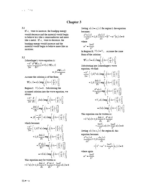
Chapter 33.1If o a were to increase, the bandgap energy would decrease and the material would begin to behave less like a semiconductor and more like a metal. If o a were to decrease, the bandgap energy would increase and thematerial would begin to behave more like an insulator._______________________________________ 3.2Schrodinger's wave equation is:()()()t x x V xt x m ,,2222ψ⋅+∂ψ∂- ()tt x j ∂ψ∂=, Assume the solution is of the form:()()⎥⎥⎦⎤⎢⎢⎣⎡⎪⎪⎭⎫ ⎝⎛⎪⎭⎫ ⎝⎛-=ψt E kx j x u t x exp , Region I: ()0=x V . Substituting theassumed solution into the wave equation, we obtain:()⎥⎥⎦⎤⎢⎢⎣⎡⎪⎪⎭⎫ ⎝⎛⎪⎭⎫ ⎝⎛-⎩⎨⎧∂∂-t E kx j x jku x m exp 22 ()⎪⎭⎪⎬⎫⎥⎥⎦⎤⎢⎢⎣⎡⎪⎪⎭⎫ ⎝⎛⎪⎭⎫ ⎝⎛-∂∂+t E kx j x x u exp ()⎥⎥⎦⎤⎢⎢⎣⎡⎪⎪⎭⎫ ⎝⎛⎪⎭⎫ ⎝⎛-⋅⎪⎭⎫ ⎝⎛-=t E kx j x u jE j exp which becomes()()⎥⎥⎦⎤⎢⎢⎣⎡⎪⎪⎭⎫ ⎝⎛⎪⎭⎫ ⎝⎛-⎩⎨⎧-t E kx j x u jk m exp 222 ()⎥⎥⎦⎤⎢⎢⎣⎡⎪⎪⎭⎫ ⎝⎛⎪⎭⎫ ⎝⎛-∂∂+t E kx j x x u jkexp 2 ()⎪⎭⎪⎬⎫⎥⎥⎦⎤⎢⎢⎣⎡⎪⎪⎭⎫ ⎝⎛⎪⎭⎫ ⎝⎛-∂∂+t E kx j x x u exp 22 ()⎥⎥⎦⎤⎢⎢⎣⎡⎪⎪⎭⎫ ⎝⎛⎪⎭⎫ ⎝⎛-+=t E kx j x Eu exp This equation may be written as()()()()0222222=+∂∂+∂∂+-x u mE x x u x x u jk x u kSetting ()()x u x u 1= for region I, the equation becomes:()()()()021221212=--+x u k dx x du jk dxx u d α where222mE=αIn Region II, ()O V x V =. Assume the same form of the solution:()()⎥⎥⎦⎤⎢⎢⎣⎡⎪⎪⎭⎫ ⎝⎛⎪⎭⎫ ⎝⎛-=ψt E kx j x u t x exp , Substituting into Schrodinger's wave equation, we find:()()⎥⎥⎦⎤⎢⎢⎣⎡⎪⎪⎭⎫ ⎝⎛⎪⎭⎫ ⎝⎛-⎩⎨⎧-t E kx j x u jk m exp 222 ()⎥⎥⎦⎤⎢⎢⎣⎡⎪⎪⎭⎫ ⎝⎛⎪⎭⎫ ⎝⎛-∂∂+t E kx j x x u jkexp 2 ()⎪⎭⎪⎬⎫⎥⎥⎦⎤⎢⎢⎣⎡⎪⎪⎭⎫ ⎝⎛⎪⎭⎫ ⎝⎛-∂∂+t E kx j x x u exp 22 ()⎥⎥⎦⎤⎢⎢⎣⎡⎪⎪⎭⎫ ⎝⎛⎪⎭⎫ ⎝⎛-+t E kx j x u V O exp ()⎥⎥⎦⎤⎢⎢⎣⎡⎪⎪⎭⎫ ⎝⎛⎪⎭⎫ ⎝⎛-=t E kx j x Eu exp This equation can be written as:()()()2222x x u x x u jk x u k ∂∂+∂∂+- ()()02222=+-x u mEx u mV OSetting ()()x u x u 2= for region II, this equation becomes()()dx x du jk dxx u d 22222+ ()022222=⎪⎪⎭⎫ ⎝⎛+--x u mV k O α where again222mE=α_______________________________________3.3We have()()()()021221212=--+x u k dx x du jk dxx u d α Assume the solution is of the form: ()()[]x k j A x u -=αexp 1()[]x k j B +-+αexp The first derivative is()()()[]x k j A k j dxx du --=ααexp 1 ()()[]x k j B k j +-+-ααexp and the second derivative becomes()()[]()[]x k j A k j dxx u d --=ααexp 2212 ()[]()[]x k j B k j +-++ααexp 2Substituting these equations into the differential equation, we find()()[]x k j A k ---ααexp 2()()[]x k j B k +-+-ααexp 2(){()[]x k j A k j jk --+ααexp 2()()[]}x k j B k j +-+-ααexp ()()[]{x k j A k ---ααexp 22 ()[]}0exp =+-+x k j B α Combining terms, we obtain()()()[]222222αααα----+--k k k k k ()[]x k j A -⨯αexp()()()[]222222αααα--++++-+k k k k k ()[]0exp =+-⨯x k j B α We find that 00=For the differential equation in ()x u 2 and the proposed solution, the procedure is exactly the same as above._______________________________________ 3.4We have the solutions ()()[]x k j A x u -=αexp 1()[]x k j B +-+αexp for a x <<0 and()()[]x k j C x u -=βexp 2()[]x k j D +-+βexp for 0<<-x b .The first boundary condition is ()()0021u u =which yields0=--+D C B AThe second boundary condition is201===x x dx dudx du which yields()()()C k B k A k --+--βαα()0=++D k β The third boundary condition is ()()b u a u -=21 which yields()[]()[]a k j B a k j A +-+-ααexp exp ()()[]b k j C --=βexp()()[]b k j D -+-+βexp and can be written as()[]()[]a k j B a k j A +-+-ααexp exp ()[]b k j C ---βexp()[]0exp =+-b k j D β The fourth boundary condition isbx a x dx dudx du -===21 which yields()()[]a k j A k j --ααexp()()[]a k j B k j +-+-ααexp ()()()[]b k j C k j ---=ββexp()()()[]b k j D k j -+-+-ββexp and can be written as ()()[]a k j A k --ααexp()()[]a k j B k +-+-ααexp()()[]b k j C k ----ββexp()()[]0exp =+++b k j D k ββ_______________________________________ 3.5(b) (i) First point: πα=aSecond point: By trial and error, πα729.1=a (ii) First point: πα2=aSecond point: By trial and error, πα617.2=a_______________________________________3.6(b) (i) First point: πα=aSecond point: By trial and error, πα515.1=a (ii) First point: πα2=aSecond point: By trial and error, πα375.2=a_______________________________________ 3.7ka a aaP cos cos sin =+'αααLet y ka =, x a =α Theny x x xP cos cos sin =+'Consider dy dof this function.()[]{}y x x x P dyd sin cos sin 1-=+⋅'- We find()()()⎭⎬⎫⎩⎨⎧⋅+⋅-'--dy dx x x dy dx x x P cos sin 112y dydxx sin sin -=- Theny x x x x x P dy dx sin sin cos sin 12-=⎭⎬⎫⎩⎨⎧-⎥⎦⎤⎢⎣⎡+-'For πn ka y ==, ...,2,1,0=n 0sin =⇒y So that, in general,()()dk d ka d a d dy dxαα===0 And22 mE=αSodk dEm mE dk d ⎪⎭⎫ ⎝⎛⎪⎭⎫ ⎝⎛=-22/122221 α This implies thatdk dE dk d ==0α for an k π= _______________________________________ 3.8(a) πα=a 1π=⋅a E m o 212()()()()2103123422221102.41011.9210054.12---⨯⨯⨯==ππa m E o19104114.3-⨯=J From Problem 3.5 πα729.12=aπ729.1222=⋅a E m o()()()()2103123422102.41011.9210054.1729.1---⨯⨯⨯=πE18100198.1-⨯=J 12E E E -=∆1918104114.3100198.1--⨯-⨯= 19107868.6-⨯=Jor 24.4106.1107868.61919=⨯⨯=∆--E eV(b) πα23=aπ2223=⋅a E m o()()()()2103123423102.41011.9210054.12---⨯⨯⨯=πE18103646.1-⨯=J From Problem 3.5, πα617.24=aπ617.2224=⋅a E m o()()()()2103123424102.41011.9210054.1617.2---⨯⨯⨯=πE18103364.2-⨯=J 34E E E -=∆1818103646.1103364.2--⨯-⨯= 1910718.9-⨯=Jor 07.6106.110718.91919=⨯⨯=∆--E eV_______________________________________3.9(a) At π=ka , πα=a 1π=⋅a E m o 212()()()()2103123421102.41011.9210054.1---⨯⨯⨯=πE19104114.3-⨯=JAt 0=ka , By trial and error, πα859.0=a o ()()()()210312342102.41011.9210054.1859.0---⨯⨯⨯=πoE19105172.2-⨯=J o E E E -=∆11919105172.2104114.3--⨯-⨯= 2010942.8-⨯=Jor 559.0106.110942.81920=⨯⨯=∆--E eV (b) At π2=ka , πα23=aπ2223=⋅a E m o()()()()2103123423102.41011.9210054.12---⨯⨯⨯=πE18103646.1-⨯=JAt π=ka . From Problem 3.5, πα729.12=aπ729.1222=⋅a E m o()()()()2103123422102.41011.9210054.1729.1---⨯⨯⨯=πE18100198.1-⨯=J23E E E -=∆1818100198.1103646.1--⨯-⨯= 19104474.3-⨯=Jor 15.2106.1104474.31919=⨯⨯=∆--E eV_______________________________________3.10(a) πα=a 1π=⋅a E m o 212()()()()2103123421102.41011.9210054.1---⨯⨯⨯=πE19104114.3-⨯=JFrom Problem 3.6, πα515.12=aπ515.1222=⋅a E m o()()()()2103123422102.41011.9210054.1515.1---⨯⨯⨯=πE1910830.7-⨯=J 12E E E -=∆1919104114.310830.7--⨯-⨯= 19104186.4-⨯=Jor 76.2106.1104186.41919=⨯⨯=∆--E eV (b) πα23=aπ2223=⋅a E m o()()()()2103123423102.41011.9210054.12---⨯⨯⨯=πE18103646.1-⨯=JFrom Problem 3.6, πα375.24=aπ375.2224=⋅a E m o()()()()2103123424102.41011.9210054.1375.2---⨯⨯⨯=πE18109242.1-⨯=J 34E E E -=∆1818103646.1109242.1--⨯-⨯= 1910597.5-⨯=Jor 50.3106.110597.51919=⨯⨯=∆--E eV_____________________________________3.11(a) At π=ka , πα=a 1π=⋅a E m o 212()()()()2103123421102.41011.9210054.1---⨯⨯⨯=πE19104114.3-⨯=JAt 0=ka , By trial and error, πα727.0=a oπ727.022=⋅a E m o o()()()()210312342102.41011.9210054.1727.0---⨯⨯⨯=πo E19108030.1-⨯=Jo E E E -=∆11919108030.1104114.3--⨯-⨯= 19106084.1-⨯=Jor 005.1106.1106084.11919=⨯⨯=∆--E eV (b) At π2=ka , πα23=aπ2223=⋅a E m o()()()()2103123423102.41011.9210054.12---⨯⨯⨯=πE18103646.1-⨯=JAt π=ka , From Problem 3.6,πα515.12=aπ515.1222=⋅a E m o()()()()2103423422102.41011.9210054.1515.1---⨯⨯⨯=πE1910830.7-⨯=J23E E E -=∆191810830.7103646.1--⨯-⨯= 1910816.5-⨯=Jor 635.3106.110816.51919=⨯⨯=∆--E eV_______________________________________3.12For 100=T K, ()()⇒+⨯-=-1006361001073.4170.124gE164.1=g E eV200=T K, 147.1=g E eV 300=T K, 125.1=g E eV 400=T K, 097.1=g E eV 500=T K, 066.1=g E eV 600=T K, 032.1=g E eV_______________________________________3.13The effective mass is given by1222*1-⎪⎪⎭⎫⎝⎛⋅=dk E d mWe have()()B curve dkE d A curve dk E d 2222> so that ()()B curve m A curve m **<_______________________________________ 3.14The effective mass for a hole is given by1222*1-⎪⎪⎭⎫ ⎝⎛⋅=dk E d m p We have that()()B curve dkEd A curve dk E d 2222> so that ()()B curve m A curve m p p **<_______________________________________ 3.15Points A,B: ⇒<0dk dEvelocity in -x directionPoints C,D: ⇒>0dk dEvelocity in +x directionPoints A,D: ⇒<022dk Ednegative effective massPoints B,C: ⇒>022dkEd positive effective mass _______________________________________3.16For A: 2k C E i =At 101008.0+⨯=k m 1-, 05.0=E eV Or ()()2119108106.105.0--⨯=⨯=E J So ()2101211008.0108⨯=⨯-C3811025.1-⨯=⇒CNow ()()38234121025.1210054.12--*⨯⨯==C m 311044.4-⨯=kgor o m m ⋅⨯⨯=--*31311011.9104437.4o m m 488.0=* For B: 2k C E i =At 101008.0+⨯=k m 1-, 5.0=E eV Or ()()2019108106.15.0--⨯=⨯=E JSo ()2101201008.0108⨯=⨯-C 3711025.1-⨯=⇒CNow ()()37234121025.1210054.12--*⨯⨯==C m 321044.4-⨯=kg or o m m ⋅⨯⨯=--*31321011.9104437.4o m m 0488.0=*_______________________________________ 3.17For A: 22k C E E -=-υ()()()2102191008.0106.1025.0⨯-=⨯--C 3921025.6-⨯=⇒C()()39234221025.6210054.12--*⨯⨯-=-=C m31108873.8-⨯-=kgor o m m ⋅⨯⨯-=--*31311011.9108873.8o m m 976.0--=* For B: 22k C E E -=-υ()()()2102191008.0106.13.0⨯-=⨯--C 382105.7-⨯=⇒C()()3823422105.7210054.12--*⨯⨯-=-=C m3210406.7-⨯-=kgor o m m ⋅⨯⨯-=--*31321011.910406.7o m m 0813.0-=*_______________________________________ 3.18(a) (i) νh E =or ()()341910625.6106.142.1--⨯⨯==h E ν1410429.3⨯=Hz(ii) 141010429.3103⨯⨯===νλc E hc 51075.8-⨯=cm 875=nm(b) (i) ()()341910625.6106.112.1--⨯⨯==h E ν1410705.2⨯=Hz(ii) 141010705.2103⨯⨯==νλc410109.1-⨯=cm 1109=nm_______________________________________ 3.19(c) Curve A: Effective mass is a constantCurve B: Effective mass is positive around 0=k , and is negativearound 2π±=k . _______________________________________ 3.20()[]O O k k E E E --=αcos 1 Then()()()[]O k k E dkdE ---=ααsin 1()[]O k k E -+=ααsin 1 and()[]O k k E dk E d -=ααcos 2122Then221222*11 αE dk Ed m o k k =⋅== or212*αE m =_______________________________________ 3.21(a) ()[]3/123/24lt dn m m m =*()()[]3/123/264.1082.04oom m =o dn m m 56.0=*(b)o o l t cnm m m m m 64.11082.02123+=+=*oo m m 6098.039.24+=o cn m m 12.0=*_______________________________________ 3.22(a) ()()[]3/22/32/3lh hh dp m m m +=*()()[]3/22/32/3082.045.0o om m +=[]o m ⋅+=3/202348.030187.0o dp m m 473.0=*(b) ()()()()2/12/12/32/3lh hh lh hh cpm m m m m ++=*()()()()om ⋅++=2/12/12/32/3082.045.0082.045.0 o cp m m 34.0=*_______________________________________ 3.23For the 3-dimensional infinite potential well, ()0=x V when a x <<0, a y <<0, and a z <<0. In this region, the wave equation is:()()()222222,,,,,,z z y x y z y x x z y x ∂∂+∂∂+∂∂ψψψ()0,,22=+z y x mEψ Use separation of variables technique, so let ()()()()z Z y Y x X z y x =,,ψSubstituting into the wave equation, we have222222zZXY y Y XZ x X YZ ∂∂+∂∂+∂∂ 022=⋅+XYZ mEDividing by XYZ , we obtain021*********=+∂∂⋅+∂∂⋅+∂∂⋅ mEz Z Z y Y Y x X XLet01222222=+∂∂⇒-=∂∂⋅X k x X k x X X xx The solution is of the form: ()x k B x k A x X x x cos sin +=Since ()0,,=z y x ψ at 0=x , then ()00=X so that 0=B .Also, ()0,,=z y x ψ at a x =, so that ()0=a X . Then πx x n a k = where ...,3,2,1=x n Similarly, we have2221y k y Y Y -=∂∂⋅ and 2221z k zZ Z -=∂∂⋅From the boundary conditions, we find πy y n a k = and πz z n a k =where...,3,2,1=y n and ...,3,2,1=z n From the wave equation, we can write022222=+---mE k k k z y xThe energy can be written as()222222⎪⎭⎫⎝⎛++==a n n n m E E z y x n n n z y x π _______________________________________ 3.24The total number of quantum states in the 3-dimensional potential well is given (in k-space) by()332a dk k dk k g T ⋅=ππ where222 mEk =We can then writemEk 2=Taking the differential, we obtaindE Em dE E m dk ⋅⋅=⋅⋅⋅⋅=2112121 Substituting these expressions into the density of states function, we have()dE E mmE a dE E g T ⋅⋅⋅⎪⎭⎫ ⎝⎛=212233 ππ Noting thatπ2h=this density of states function can be simplified and written as()()dE E m h a dE E g T ⋅⋅=2/33324π Dividing by 3a will yield the density of states so that()()E h m E g ⋅=32/324π _______________________________________ 3.25For a one-dimensional infinite potential well,222222k a n E m n ==*π Distance between quantum states()()aa n a n k k n n πππ=⎪⎭⎫ ⎝⎛=⎪⎭⎫ ⎝⎛+=-+11Now()⎪⎭⎫ ⎝⎛⋅=a dkdk k g T π2NowE m k n *⋅=21dE Em dk n⋅⋅⋅=*2211 Then()dE Em a dE E g n T ⋅⋅⋅=*2212 π Divide by the "volume" a , so ()Em E g n *⋅=21πSo()()()()()EE g 31341011.9067.0210054.11--⨯⋅⨯=π ()EE g 1810055.1⨯=m 3-J 1-_______________________________________ 3.26(a) Silicon, o n m m 08.1=*()()c nc E E h m E g -=*32/324π()dE E E h m g kTE E c nc c c⋅-=⎰+*232/324π()()kT E E c nc cE E h m 22/332/33224+*-⋅⋅=π()()2/332/323224kT hm n⋅⋅=*π ()()[]()()2/33342/33123210625.61011.908.124kT ⋅⋅⨯⨯=--π ()()2/355210953.7kT ⨯=(i) At 300=T K, 0259.0=kT eV()()19106.10259.0-⨯= 2110144.4-⨯=J Then ()()[]2/3215510144.4210953.7-⨯⨯=c g25100.6⨯=m 3-or 19100.6⨯=c g cm 3-(ii) At 400=T K, ()⎪⎭⎫⎝⎛=3004000259.0kT034533.0=eV()()19106.1034533.0-⨯= 21105253.5-⨯=J Then()()[]2/32155105253.5210953.7-⨯⨯=c g2510239.9⨯=m 3- or 191024.9⨯=c g cm 3-(b) GaAs, o nm m 067.0=*()()[]()()2/33342/33123210625.61011.9067.024kT g c ⋅⋅⨯⨯=--π ()()2/3542102288.1kT ⨯=(i) At 300=T K, 2110144.4-⨯=kT J ()()[]2/3215410144.42102288.1-⨯⨯=c g2310272.9⨯=m 3- or 171027.9⨯=c g cm 3-(ii) At 400=T K, 21105253.5-⨯=kT J ()()[]2/32154105253.52102288.1-⨯⨯=c g2410427.1⨯=m 3-181043.1⨯=c g cm 3-_______________________________________ 3.27(a) Silicon, o p m m 56.0=* ()()E E h mE g p-=*υυπ32/324()dE E E h mg E kTE p⋅-=⎰-*υυυυπ332/324()()υυυπE kTE pE E hm 32/332/33224-*-⎪⎭⎫ ⎝⎛-=()()[]2/332/333224kT hmp-⎪⎭⎫ ⎝⎛-=*π ()()[]()()2/33342/33133210625.61011.956.024kT ⎪⎭⎫ ⎝⎛⨯⨯=--π ()()2/355310969.2kT ⨯=(i)At 300=T K, 2110144.4-⨯=kT J ()()[]2/3215510144.4310969.2-⨯⨯=υg2510116.4⨯=m3-or 191012.4⨯=υg cm 3- (ii)At 400=T K, 21105253.5-⨯=kT J()()[]2/32155105253.5310969.2-⨯⨯=υg2510337.6⨯=m3-or 191034.6⨯=υg cm 3- (b) GaAs, o p m m 48.0=*()()[]()()2/33342/33133210625.61011.948.024kT g ⎪⎭⎫ ⎝⎛⨯⨯=--πυ ()()2/3553103564.2kT ⨯=(i)At 300=T K, 2110144.4-⨯=kT J()()[]2/3215510144.43103564.2-⨯⨯=υg2510266.3⨯=m 3- or 191027.3⨯=υg cm 3-(ii)At 400=T K, 21105253.5-⨯=kT J()()[]2/32155105253.53103564.2-⨯⨯=υg2510029.5⨯=m 3-or 191003.5⨯=υg cm 3-_______________________________________ 3.28(a) ()()c nc E E h m E g -=*32/324π()()[]()c E E -⨯⨯=--3342/33110625.61011.908.124πc E E -⨯=56101929.1 For c E E =; 0=c g1.0+=c E E eV; 4610509.1⨯=c g m 3-J 1-2.0+=c E E eV; 4610134.2⨯=m 3-J 1-3.0+=c E E eV; 4610614.2⨯=m 3-J 1- 4.0+=c E E eV; 4610018.3⨯=m 3-J 1- (b) ()E E h m g p-=*υυπ32/324()()[]()E E -⨯⨯=--υπ3342/33110625.61011.956.024E E -⨯=υ55104541.4 For υE E =; 0=υg1.0-=υE E eV; 4510634.5⨯=υg m 3-J 1-2.0-=υE E eV; 4510968.7⨯=m 3-J 1-3.0-=υE E eV; 4510758.9⨯=m 3-J 1-4.0-=υE E eV; 4610127.1⨯=m 3-J 1-_______________________________________ 3.29(a) ()()68.256.008.12/32/32/3=⎪⎭⎫ ⎝⎛==**pnc m m g g υ(b) ()()0521.048.0067.02/32/32/3=⎪⎭⎫ ⎝⎛==**pncmm g g υ_______________________________________3.30 Plot_______________________________________ 3.31(a) ()()()!710!7!10!!!-=-=i i i i i N g N g W()()()()()()()()()()()()1201238910!3!7!78910===(b) (i) ()()()()()()()()12!10!101112!1012!10!12=-=i W 66=(ii) ()()()()()()()()()()()()1234!8!89101112!812!8!12=-=i W 495=_______________________________________ 3.32()⎪⎪⎭⎫ ⎝⎛-+=kT E E E f F exp 11(a) kT E E F =-, ()()⇒+=1exp 11E f()269.0=E f (b) kT E E F 5=-, ()()⇒+=5exp 11E f()31069.6-⨯=E f(c) kT E E F 10=-, ()()⇒+=10exp 11E f ()51054.4-⨯=E f_______________________________________ 3.33()⎪⎪⎭⎫ ⎝⎛-+-=-kT E E E f F exp 1111or()⎪⎪⎭⎫ ⎝⎛-+=-kT E E E f F exp 111(a) kT E E F =-, ()269.01=-E f (b) kT E E F 5=-, ()31069.61-⨯=-E f(c) kT E E F 10=-, ()51054.41-⨯=-E f_______________________________________ 3.34(a) ()⎥⎦⎤⎢⎣⎡--≅kT E E f F F exp c E E =; 61032.90259.030.0exp -⨯=⎥⎦⎤⎢⎣⎡-=F f 2kT E c +; ()⎥⎦⎤⎢⎣⎡+-=0259.020259.030.0exp F f 61066.5-⨯=kT E c +; ()⎥⎦⎤⎢⎣⎡+-=0259.00259.030.0exp F f 61043.3-⨯=23kT E c +; ()()⎥⎦⎤⎢⎣⎡+-=0259.020259.0330.0exp F f 61008.2-⨯=kT E c 2+; ()()⎥⎦⎤⎢⎣⎡+-=0259.00259.0230.0exp F f 61026.1-⨯=(b) ⎥⎦⎤⎢⎣⎡-+-=-kT E E f F F exp 1111()⎥⎦⎤⎢⎣⎡--≅kT E E F exp υE E =; ⎥⎦⎤⎢⎣⎡-=-0259.025.0exp 1F f 51043.6-⨯= 2kT E -υ; ()⎥⎦⎤⎢⎣⎡+-=-0259.020259.025.0exp 1F f 51090.3-⨯=kT E -υ; ()⎥⎦⎤⎢⎣⎡+-=-0259.00259.025.0exp 1F f 51036.2-⨯=23kTE -υ; ()()⎥⎦⎤⎢⎣⎡+-=-0259.020259.0325.0exp 1F f 51043.1-⨯= kT E 2-υ;()()⎥⎦⎤⎢⎣⎡+-=-0259.00259.0225.0exp 1F f 61070.8-⨯=_______________________________________3.35()()⎥⎦⎤⎢⎣⎡-+-=⎥⎦⎤⎢⎣⎡--=kT E kT E kT E E f F c F F exp exp and()⎥⎦⎤⎢⎣⎡--=-kT E E f F F exp 1 ()()⎥⎦⎤⎢⎣⎡---=kT kT E E F υexp So ()⎥⎦⎤⎢⎣⎡-+-kT E kT E F c exp ()⎥⎦⎤⎢⎣⎡+--=kT kT E E F υexp Then kT E E E kT E F F c +-=-+υOr midgap c F E E E E =+=2υ_______________________________________ 3.3622222ma n E n π =For 6=n , Filled state()()()()()2103122234610121011.92610054.1---⨯⨯⨯=πE18105044.1-⨯=Jor 40.9106.1105044.119186=⨯⨯=--E eV For 7=n , Empty state ()()()()()2103122234710121011.92710054.1---⨯⨯⨯=πE1810048.2-⨯=Jor 8.12106.110048.219187=⨯⨯=--E eV Therefore 8.1240.9<<F E eV_______________________________________ 3.37(a) For a 3-D infinite potential well()222222⎪⎭⎫ ⎝⎛++=a n n n mE z y x π For 5 electrons, the 5th electron occupies the quantum state 1,2,2===z y x n n n ; so()2222252⎪⎭⎫ ⎝⎛++=a n n n m E z y x π()()()()()21031222223410121011.9212210054.1---⨯⨯++⨯=π1910761.3-⨯=Jor 35.2106.110761.319195=⨯⨯=--E eV For the next quantum state, which is empty, the quantum state is 2,2,1===z y x n n n . This quantum state is at the same energy, so 35.2=F E eV(b) For 13 electrons, the 13th electronoccupies the quantum state 3,2,3===z y x n n n ; so ()()()()()2103122222341310121011.9232310054.1---⨯⨯++⨯=πE 1910194.9-⨯=Jor 746.5106.110194.9191913=⨯⨯=--E eVThe 14th electron would occupy the quantum state 3,3,2===z y x n n n . This state is at the same energy, so 746.5=F E eV_______________________________________ 3.38The probability of a state at E E E F ∆+=1 being occupied is()⎪⎭⎫ ⎝⎛∆+=⎪⎪⎭⎫ ⎝⎛-+=kT E kT E E E f F exp 11exp 11111 The probability of a state at E E E F ∆-=2being empty is()⎪⎪⎭⎫ ⎝⎛-+-=-kT E E E f F 222exp 1111⎪⎭⎫ ⎝⎛∆-+⎪⎭⎫ ⎝⎛∆-=⎪⎭⎫ ⎝⎛∆-+-=kT E kT E kT E exp 1exp exp 111or()⎪⎭⎫ ⎝⎛∆+=-kT E E f exp 11122so ()()22111E f E f -=_______________________________________3.39(a) At energy 1E , we want01.0exp 11exp 11exp 1111=⎪⎪⎭⎫ ⎝⎛-+⎪⎪⎭⎫ ⎝⎛-+-⎪⎪⎭⎫ ⎝⎛-kT E E kT E E kT E E F F FThis expression can be written as01.01exp exp 111=-⎪⎪⎭⎫ ⎝⎛-⎪⎪⎭⎫ ⎝⎛-+kT E E kT E E F F or()⎪⎪⎭⎫⎝⎛-=kT E E F 1exp 01.01Then()100ln 1kT E E F += orkT E E F 6.41+= (b)At kT E E F 6.4+=, ()()6.4exp 11exp 1111+=⎪⎪⎭⎫ ⎝⎛-+=kT E E E f F which yields()01.000990.01≅=E f_______________________________________ 3.40 (a)()()⎥⎦⎤⎢⎣⎡--=⎥⎦⎤⎢⎣⎡--=0259.050.580.5exp exp kT E E f F F 61032.9-⨯=(b) ()060433.03007000259.0=⎪⎭⎫⎝⎛=kT eV31098.6060433.030.0exp -⨯=⎥⎦⎤⎢⎣⎡-=F f (c) ()⎥⎦⎤⎢⎣⎡--≅-kT E E f F F exp 1 ⎥⎦⎤⎢⎣⎡-=kT 25.0exp 02.0or 5002.0125.0exp ==⎥⎦⎤⎢⎣⎡+kT ()50ln 25.0=kTor()()⎪⎭⎫⎝⎛===3000259.0063906.050ln 25.0T kT which yields 740=T K_______________________________________ 3.41 (a)()00304.00259.00.715.7exp 11=⎪⎭⎫ ⎝⎛-+=E for 0.304%(b) At 1000=T K, 08633.0=kT eV Then()1496.008633.00.715.7exp 11=⎪⎭⎫ ⎝⎛-+=E for 14.96%(c) ()997.00259.00.785.6exp 11=⎪⎭⎫ ⎝⎛-+=E for 99.7% (d)At F E E =, ()21=E f for all temperatures_______________________________________ 3.42(a) For 1E E =()()⎥⎦⎤⎢⎣⎡--≅⎪⎪⎭⎫ ⎝⎛-+=kT E E kTE E E fF F11exp exp 11Then()611032.90259.030.0exp -⨯=⎪⎭⎫ ⎝⎛-=E fFor 2E E =, 82.030.012.12=-=-E E F eV Then()⎪⎭⎫ ⎝⎛-+-=-0259.082.0exp 1111E for()⎥⎦⎤⎢⎣⎡⎪⎭⎫ ⎝⎛---≅-0259.082.0exp 111E f141078.10259.082.0exp -⨯=⎪⎭⎫ ⎝⎛-=(b) For 4.02=-E E F eV,72.01=-F E E eVAt 1E E =,()()⎪⎭⎫⎝⎛-=⎥⎦⎤⎢⎣⎡--=0259.072.0exp exp 1kT E E E f F or()131045.8-⨯=E f At 2E E =,()()⎥⎦⎤⎢⎣⎡--=-kT E E E f F 2exp 1 ⎪⎭⎫ ⎝⎛-=0259.04.0expor()71096.11-⨯=-E f_______________________________________ 3.43(a) At 1E E =()()⎪⎭⎫⎝⎛-=⎥⎦⎤⎢⎣⎡--=0259.030.0exp exp 1kT E E E f F or()61032.9-⨯=E fAt 2E E =, 12.13.042.12=-=-E E F eV So()()⎥⎦⎤⎢⎣⎡--=-kT E E E f F 2exp 1 ⎪⎭⎫ ⎝⎛-=0259.012.1expor()191066.11-⨯=-E f (b) For 4.02=-E E F ,02.11=-F E E eV At 1E E =,()()⎪⎭⎫⎝⎛-=⎥⎦⎤⎢⎣⎡--=0259.002.1exp exp 1kT E E E f F or()181088.7-⨯=E f At 2E E =,()()⎥⎦⎤⎢⎣⎡--=-kT E E E f F 2exp 1 ⎪⎭⎫ ⎝⎛-=0259.04.0expor ()71096.11-⨯=-E f_______________________________________ 3.44()1exp 1-⎥⎦⎤⎢⎣⎡⎪⎪⎭⎫ ⎝⎛-+=kTE E E f Fso()()2exp 11-⎥⎦⎤⎢⎣⎡⎪⎪⎭⎫ ⎝⎛-+-=kT E E dE E df F⎪⎪⎭⎫ ⎝⎛-⎪⎭⎫⎝⎛⨯kT E E kT F exp 1or()2exp 1exp 1⎥⎦⎤⎢⎣⎡⎪⎪⎭⎫ ⎝⎛-+⎪⎪⎭⎫ ⎝⎛-⎪⎭⎫⎝⎛-=kT E E kT E E kT dE E df F F (a) At 0=T K, For()00exp =⇒=∞-⇒<dE dfE E F()0exp =⇒+∞=∞+⇒>dEdfE E FAt -∞=⇒=dEdfE E F(b) At 300=T K, 0259.0=kT eVFor F E E <<, 0=dE dfFor F E E >>, 0=dEdfAt F E E =,()()65.91110259.012-=+⎪⎭⎫ ⎝⎛-=dE df (eV)1-(c) At 500=T K, 04317.0=kT eVFor F E E <<, 0=dE dfFor F E E >>, 0=dEdfAt F E E =,()()79.511104317.012-=+⎪⎭⎫ ⎝⎛-=dE df (eV)1- _______________________________________ 3.45(a) At midgap E E =,()⎪⎪⎭⎫⎝⎛+=⎪⎪⎭⎫ ⎝⎛-+=kT E kTE E E f g F2exp 11exp 11Si: 12.1=g E eV, ()()⎥⎦⎤⎢⎣⎡+=0259.0212.1exp 11E for()101007.4-⨯=E fGe: 66.0=g E eV ()()⎥⎦⎤⎢⎣⎡+=0259.0266.0exp 11E for()61093.2-⨯=E f GaAs: 42.1=g E eV ()()⎥⎦⎤⎢⎣⎡+=0259.0242.1exp 11E for()121024.1-⨯=E f(b) Using the results of Problem 3.38, the answers to part (b) are exactly the same as those given in part (a)._______________________________________3.46(a) ()⎥⎦⎤⎢⎣⎡--=kT E E f F F exp ⎥⎦⎤⎢⎣⎡-=-kT 60.0exp 108or()810ln 60.0+=kT()032572.010ln 60.08==kT eV ()⎪⎭⎫⎝⎛=3000259.0032572.0Tso 377=T K(b) ⎥⎦⎤⎢⎣⎡-=-kT 60.0exp 106()610ln 60.0+=kT()043429.010ln 60.06==kT ()⎪⎭⎫⎝⎛=3000259.0043429.0Tor 503=T K_______________________________________ 3.47(a) At 200=T K,()017267.03002000259.0=⎪⎭⎫⎝⎛=kT eV⎪⎪⎭⎫ ⎝⎛-+==kT E E f F F exp 1105.019105.01exp =-=⎪⎪⎭⎫ ⎝⎛-kT E E F()()()19ln 017267.019ln ==-kT E E F 05084.0=eV By symmetry, for 95.0=F f , 05084.0-=-F E E eVThen ()1017.005084.02==∆E eV (b) 400=T K, 034533.0=kT eV For 05.0=F f , from part (a),()()()19ln 034533.019ln ==-kT E E F 10168.0=eVThen ()2034.010168.02==∆E eV _______________________________________。

第四章 金属-半导体结4-1. 一硅肖脱基势垒二极管有0.01 cm 2的接触面积,半导体中施主浓度为1016 cm 3−。
设V 7.00=ψ,V V R 3.10=。
计算 (a )耗尽层厚度,(b )势垒电容,(c )在表面处的电场4-2. (a )从示于图4-3的GaAs 肖脱基二极管电容-电压曲线求出它的施主浓度、自建电势势垒高度。
(b) 从图4-7计算势垒高度并与(a )的结果作比较。
4-3. 画出金属在P 型半导体上的肖脱基势垒的能带结构图,忽略表面态,指出(a )s m φφ>和(b )s m φφ<两种情形是整流节还是非整流结,并确定自建电势和势垒高度。
4-4. 自由硅表面的施主浓度为15310cm −,均匀分布的表面态密度为122110ss D cm eV −−=,电中性级为0.3V E eV +,向该表面的表面势应为若干?提示:首先求出费米能级与电中性能级之间的能量差,存在于这些表面态中的电荷必定与表面势所承受的耗尽层电荷相等。
4-5. 已知肖脱基二极管的下列参数:V m 0.5=φ,eV s 05.4=χ,31910−=cm N c ,31510−=cm N d ,以及k=11.8。
假设界面态密度是可以忽略的,在300K 计算: (a )零偏压时势垒高度,自建电势,以及耗尽层宽度。
(b)在0.3v 的正偏压时的热离子发射电流密度。
4-6.在一金属-硅的接触中,势垒高度为eV q b 8.0=φ,有效理查逊常数为222/10*K cm A R ⋅=,eV E g 1.1=,31610−=cm N d ,以及31910−==cm N N v c 。
(a )计算在300K 零偏压时半导体的体电势n V和自建电势。
(b )假设s cm D p /152=和um L p 10=,计算多数载流子电流对少数载流子电流的注入比。
4-7. 计算室温时金-nGaAs 肖脱基势垒的多数载流子电流对少数载流子电流的比例。


Semiconductor Device PhysicsSui-Dong Wang 2010-2011Outline章 节 一 二 三 四 五 六 七 合 计 内 容 半导体器件简介 半导体晶体结构 半导体能带理论基础 P-N二极管 MOS场效应晶体管 MES场效应晶体管 半导体光电器件 周 时 1 1 3 2 2 2 5 16 授 课 王穗东 王穗东 王穗东 王穗东 王穗东 王穗东 唐建新What Is A Diode ?A two-terminal electronic component that conduct electric current in only one directionWhat Is A P-N Diode ?Depletion region Î Space charge region Î Current modulation Electric field and potential distribution?Gauss’s Law / Poisson EquationAn example: Point chargeDepletion Region in P-N JunctionDepletion Region – Electric FieldDepletion Region – PotentialDepletion Region – PotentialOne-side P-N JunctionWDHeavily-doped P++Lightly-doped NDebye LengthThe Debye length LD, is a characteristic length for semiconductors and is defined as:At thermal equilibrium the depletion-layer widths of abrupt junctions are about 8LD for Si, and 10LD for GaAs.Linearly Graded P-N JunctionLinearly Graded P-N JunctionLinearly Graded P-N JunctionP-N Junction under Forward BiasDepletion layer width ? Build-in potential ? Current ?P-N Junction under Reverse BiasDepletion layer width ? Build-in potential ? Current ?I-V Characteristics of P-N JunctionReverse breakdown mechanism?Breakdown Mechanism - TunnelingBreakdown Mechanism Avalanche MultiplicationImpact ionization under high electric fieldApplications - Diode TypesApplications -RectifierRectifier gives a very low resistance to current flow inone direction and a very high resistance in the other direction.Applications -Zener DiodeZener breakdown occurs at a precisely defined voltage, allowing the diode to be used as a precision voltage reference.Applications -VaristorVaristor shows non-ohmic voltage-dependent resistance.Applications -Varactor Varactor works at reverse bias acting as a capacitor.Applications -Tunnel DiodeTunnel diode is heavily doped with narrow depletion region.Applications -Photodiode Photodiode works as a switch controlled by light.Applications -Light Emitting Diode Light emitting diode emits light under electrical bias.Questions(1)How to calculate energy potential in a space chargeregion in semiconductors ?(2)How do you understand the physical term“Junction”? Homojunction ? Heterojunction ?。