转子动力学分析72页PPT
- 格式:ppt
- 大小:7.13 MB
- 文档页数:72


第1章绪论1.1问题背景往复活塞式内燃机的曲轴系包括活塞、连杆、曲柄等内燃机的主要运动部件。
其功用是将活塞的往复运动转化为曲轴的旋转运动,且将作用的活塞上的燃气压力转化为扭矩,借助飞轮向外输出,从而实现热能向机械能的转化,是内燃机传递运动和动力的机器。
内燃机工作时,其机械行为表现为多学科的行为同时发生。
实际上,机械设计就是多学科的行为的综合和优化。
但以往由于计算机技术落后,计算能力有限,机械行为研究主要集中在单一的学科领域。
近年来随着对内燃机动力性和可靠性的要求不断提高,高转速、废气增压发动机的出现,使曲轴系的工作条件愈加苛刻,原有的动力学、摩擦学、强度、刚度等单学科行为研究已远不能适应现代内燃机设计的需要,迫切需求对曲轴系进行多学科行为的综合研究。
同时,随着计算技术的发展,各种专业软件的广泛应用,为曲轴系多学科机械行为的研究提供了必要的前提[1] 。
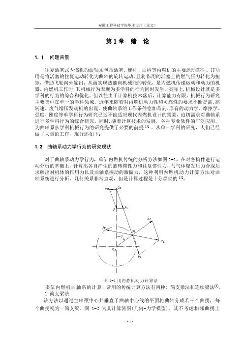
从单一学科的研究,人们已经做了大量的工作,现分述如下:1.2 曲轴系动力学行为的研究现状对于曲轴系动力学行为,单缸内燃机传统的分析方法如图1-1,在对各构件进行运动分析的基础上,计算出各自产生的旋转惯性力和往复惯性力,与气体爆发压力合成后求解出对机体的作用力以及曲轴系振动的激振力,这种利用内燃机动力计算方法对曲轴系统进行分析,几何关系非常直观,但是计算过程是十分烦琐的[1]。
图1-1用内燃机动力计算法多缸内燃机曲轴系的计算,常用的传统计算方法有两种: 简支梁法和连续梁法[2]。
1 简支梁法该方法以通过主轴颈中心并垂直于曲轴中心线的平面将曲轴分成若干个曲拐, 每个曲拐视为一简支梁。
图1-2 为其计算简图(几何-力学模型)。
其不考虑相邻曲拐上作用力的影响,与实际情况有较大差异。
图1-2 简支梁法计算简图2 连续梁法连续梁法把曲轴简化为多支承的静不定连续梁(图1-3) , 应用三弯矩或五弯矩方程求解。
由于假设的几何-力学模型不同, 连续梁法主要有以下三种:①将曲轴简化为多支承圆柱形连续直梁, 其直径与轴颈直径相同或相当;②曲轴作为支承在弹性支承上变截面的静不定直梁;③曲轴作为支承在弹性支承上的静不定曲梁。
ABSTRACTThe goals of this study were to examine the dynamic force-deformation and kinematic response of a late model van subjected to an inverted drop test and to evaluate the accuracy of three-dimensional multi-point roof deformation measurements made by an optical system mounted inside the vehicle. The inverted drop test was performed using a dynamic rollover test system (Kerrigan et al., 2011 SAE)with an initial vehicle pitch of −5 degrees, a roll of +155degrees and a vertical velocity of 2.7 m/s at initial contact.Measurements from the optical system, which was composed of two high speed imagers and a commercial optical processing software were compared to deformation measurements made by two sets of three string potentiometers. The optical and potentiometer measurements reported similar deformations: peak resultant deformations varied by 0.7 mm and 3 ms at the top of the A-pillar, and 1.7mm and 2 ms at the top of the B-pillar. The top of the vehicle B-pillar sustained peak resultant deformation of 146.2 mm 116 ms after contact, and unloaded to 77.1 mm (47% of peak)at 291 ms. Peak reaction forces at contact were approximately 100 kN, and the force-deflection response between the drop test and the IIHS roof crush test on the same make and model vehicle showed comparable dynamic and quasi-static stiffness. The results presented in this study showed that the optical system can be used to measure dynamic roof deformations, in three dimensions, at high rates, across a large area of the vehicle structure, from inside a vehicle subjected to rollover crash test.INTRODUCTIONMulti-point deformation information can be an enabler in validating vehicle finite element model predictions,examining the mechanism of rollover-crash induced injuries,and studying the type of relationship between the timing,location, and magnitude of roof deformations and occupant injury metrics.Previous research has presented roof deformation measurement techniques using string potentiometers and videogrammetry during multiple rollover events [2].However, the methods are not described in detail, the results are only presented for single points, and the two techniques are not compared to each other or any other independent deformation measurement technique.The goal of this study was to evaluate the accuracy of measurements made with a three-dimensional multi-point optical deformation measurement system in a high-rate deformation experiment. The optical approach relies on the principles of stereo videogrammetry to accurately produce three-dimensional displacement time histories for a high resolution multi-point surface. Combined with vehicle kinematics and ground reaction force time histories, the optical output could provide a powerful tool for validating vehicle finite element roof structural models as well as occupant injury metrics.To achieve these goals, an inverted vehicle drop test was performed on a late model passenger van using the University of Virginia Center for Applied Biomechanics' Dynamic Rollover Test System (DRoTS) [5]. For this test, the vehicle roll drives and sled propulsion were disabled. The test parameters were chosen to mimic the loading that occurs in the IIHS roof strength evaluation (similar to the FMVSS 216test), to allow for a force-deflection comparison between dynamic and quasi-static roof loading conditions on the same make and model vehicle.Deformation measurement was focused on the passenger side roof rail between the A-pillar and B-pillar, as this was thepoint of initial roof to ground contact and anticipated locationOptical Measurement of High-Rate Dynamic Vehicle Roof Deformation during Rollover2013-01-0470Published 04/08/2013Jack Lockerby, Jason Kerrigan, Jeremy Seppi and Jeff CrandallUVA Center for Applied BiomechanicsCopyright © 2013 SAE Internationaldoi:10.4271/2013-01-0470of maximum deformation. Two methods were used to measure the three-dimensional deformation time history of the vehicle roof structure. The optical system utilized two on-board high speed imagers and optical processing software.The second method, based on string potentiometer trilateration, was implemented at two discrete points on the A-pillar and B-pillar to validate the optical system's results.The resultant and component displacements for the A-pillar and B-pillar points were compared against the optical system's output for the same locations.The optical system incorporated ARAMIS v6 2.0 (GOM Optical Measuring Techniques), a commercially available optical measurement software package. ARAMIS utilized digital images to analyze and report three-dimensional material deformations along with the surface coordinates of points, displacements and velocities, and strain values and rates.METHODS Test ConditionsThe vehicle's as tested mass was 1911.9 kg. The initial conditions for the vehicle were a pitch angle of −5 degrees (front end down), a roll angle of +155 degrees (passenger side impact), and a drop height of 0.398 m (total vertical motion of CG prior to impact), (Figure 1). This produced a 2.706 m/s vertical velocity at contact. Unpublished finite element analysis results suggested that peak reaction force from this drop height would be approximately equal to the peak force achieved in the IIHS roof strength evaluation withthe same vehicle.Figure 1. Initial vehicle orientation for the drop test The IIHS roof strength evaluation, the quasi-static test on the vehicle used for comparison, consisted of a roof crush test to one side of the vehicle. The test system utilized an upright assembly with attached loading platen fixed at 25 degrees rolland 5 degrees of pitch [4]. The vehicle roof was crushed to a minimum of 127 mm of platen displacement at a nominal rate of 5 mm/s. Force and displacement data were reported at 100Hz for the test.Vehicle PreparationThe vehicle's overall mass and wheel distributions were measured upon delivery at UVA as the test goal weight, and monitored throughout the preparation and installation process. The vehicle fluids were drained and the seats, floor liners, roof liners, and curtain airbags were removed to allow for instrumentation installation. Steel plates were bolted to the vehicle floor to act as mounting locations for instrumentation and data acquisition equipment (Figure 2). A contact strip sensor was taped on the roof in the location of anticipated initial roof-to-ground contact as a trigger. The passenger side interior structural surfaces were painted with a stochastic pattern of black dots, 6 to 12 mm diameter with approximate 40-50% coverage of the patterned area, on awhite background to accommodate the optical system.Figure 2. Instrumentation mounting plates and sensor cube installed location on the floor pan of the vehicleBalancing ProcedureThe DRoTS cradle [5], which consisted of two vertically oriented steel tubing towers at the front and rear, connected by a set of telescoping steel tubes 5″ in diameter, was installed on the vehicle to fix the location and orientation of the vehicle's roll axis relative to the vehicle (Figure 3). It is about this roll axis that the DRoTS fixture rotates the vehicle in a typical rollover crash test (disabled for this test). Once installed, the telescoping tube ran under the vehicle body from the front to the rear and the towers were oriented perpendicular to the ground. The towers of the cradle were fixed to the vehicle frame rails in the front and rear of the vehicle by removing the fascia and bumper beams and using custom hardware to rigidly connect the towers to the locations where the bumper beams interfaced with the vehicle frame rails. The cradle assembly was centered (left-right)between the bumper beam/frame rail connections at the frontand rear of the vehicle. For simplicity, the cradle was installed such that the tube was oriented parallel with the ground when the vehicle was resting on its own suspension/tires, at the curb weight condition. The DRoTS fixture was designed to hold the vehicle cradle in such a way that the vehicle roll axis was parallel to the cradle. Once the vehicle was loaded in the test fixture, the location of the roll axis relative to the vehicle and cradle was adjusted vertically until the roll axis passed through the center of gravity (CG) of the vehicle. If the vehicle CG was not aligned in the center of the frame rails (left-right) then ballast weight was added to one side to ensure alignment. At the completion of the balancing procedure, the vehicle would not continue to rotate in either direction after being manually rotated and stopped at 45degree intervals from 0 to 360 degrees. After this adjustment was completed the exact location of the roll axis could be identified from a single marker point at the very front andrear of the cradle.Figure 3. DRoTS cradle installation on front of vehicleForce and Kinematics Measurement SensorsThe vehicle was outfitted with an inertial measurement cube containing three accelerometers (Endevco 7290E-30, Meggitt Sensing Systems, San Juan Capistrano, CA) measuring accelerations about the sensor cube's local x, y, and z component directions. Additionally three angular rate sensors were included measuring angular velocities about the same local sensor cube axes (DTS ARS-1500, Diversified Technical Systems, Seal Beach, CA) for the x direction, and two (DTS ARS-300, Diversified Technical Systems, Seal Beach, CA) for the y and z directions. The sensor cube was mounted on the floor of the vehicle, on the lateral center line (Figure 2). The DRoTS roadbed was instrumented with twenty-four uniaxial load cells, spaced evenly across the surface, and oriented to measure in the vertical direction (global Z′). Two accelerometers measuring in the vertical Z′direction were mounted to the underside of the wood surfaceat the left-front corner and right-rear corner of the center section of the roadbed.Deformation Measurement SensorsThe passenger side A-pillar and B-pillar were both instrumented with a set of three string potentiometers of 2159mm maximum travel (Firstmark Model 62, Firstmark Controls, Creedmoor, NC). Two mounting plates (25 × 50mm) were constructed out of steel stock. To each plate, a single screw and a triax accelerometer were attached (Entran Triax EGAXT3, PandAuto Technology Co., Ltd). One of the two plates was mounted on the passenger-side A-pillar, at a location approximately 150 mm from the intersection of the A-pillar, roof rail, and windshield header. The second plate was mounted on the roof rail, approximately 100 mm forwardof the B-Pillar roof rail connection (Figure 4).Figure 4. B-pillar string potentiometer attachment plateThe plates were fixed to the vehicle via a single screw inserted into existing threaded holes used for mounting the rollover curtain airbags. Rotation of each plate was prevented with a sharpened screw, inserted in the plate that was tightened against the vehicle interior at the mounting location. The strings from each of three string potentiometers were attached to the screw on each of the two plates (n= 6string potentiometers). The six string potentiometers were affixed to the floor of the vehicle via rigid steel plates attached to the driver, right front passenger and second row seat mounting locations (Figure 5).Figure 5. String potentiometer mounting and orientationOptical SystemThe optical system was comprised of two high-speed imagers (NAC GX-1, NAC Image Technology, Simi Valley, CA)with 16 mm focal length ruggedized lenses (Schneider Optics, Hauppauge, NY). The imagers were fixed at a 21degree horizontal angle with respect to each other, and mounted on a rigid aluminum camera bar along with six high intensity LED, and two laser sights tracing the center pixel of each camera for visual alignment. The camera bar was bolted onto a steel framing structure that was welded into the vehicle floor at the front row seat mounting beam (Figure 6). In the mounted orientation, the cameras shared a focal intersection point 915 mm from the lenses, which was positioned 25 mm in front of the intersection of the vehicle passenger side roof rail with the windshield header (Figure 7). Sections of the roof, roof rail, A-/B-pillars, and windshield header above thepassenger seat were included in the shared field of view.Figure 6.Figure 6 (cont). Optical system components andmounting structure on the floor pan of the vehicleFigure 7. Images from the left and right cameras at t=0ms, structure undeformedCoordinate MeasurementsA coordinate measurement machine (CMM) (Titanium Arm,FARO Technologies, Lake Mary, FL) was used to determine the locations of the front and rear roll axis marker points, side door latch plates, wheel centers, the inertial measurement cube origin and orientation markers, the locations of the string potentiometer attachment screw locations on the A-/B-pillars, the points where the strings come out of the potentiometer bases, the accelerometers mounted on the string attachment plates, and four points located in the view of the optical system. Since digitizing these points required moving the CMM around the exterior of the car, a series of overlapping points were taken in each measurement location,and each point cloud captured in each measurement location was aligned in a single coordinate system by singular value decomposition [3].Data ProcessingKinematics Data ProcessingAll sensor data were filtered and debiased. Road load cells,vehicle accelerometers, and string potentiometers, were filtered to CFC60 and vehicle angular rate sensors were filtered to CFC180 [6]. For the purpose of calculating the angular accelerations necessary for determining vehicle CG kinematics from kinematics measured at the sensor cube, theangular velocity data were filtered with a Butterworth 4-pole zero-phase low-pass digital filter with a 25 Hz cutoff. Road loads were summed to determine total vertical reaction force.The time of initial vehicle to road contact was determined to within 1 ms from high speed video, and all time history data were time shifted so that t =0 corresponded with the time of initial vehicle contact with the road surface.Once the CMM data point clouds were unified, vehicle local and global (inertial) coordinate systems were defined. A standardized SAE definition for the vehicle coordinate system was used [6]. The vehicle's positive X axis was defined by a vector directed from the rear roll axis point to the front roll axis point; the positive Y axis was defined by an average of vectors connecting similar points from the driver's side to the passenger's side door latch plates; and positive Z was determined by the cross product of X and Y vectors.These vectors were calculated in the CMM coordinate system and were used to define the rotation matrix R vehcmm .The point cloud was then rotated from the CMM coordinate system to the vehicle local coordinate system by R vehcmm and its origin was translated to the center of the line connecting the front and rear roll axis marker points. The front/rear right/left weight distribution was used, with the CMM-determined locations of the center of the wheels, to determine the location of the vehicle CG on the XY plane. Then the origin of the vehicle coordinate system was translated to the CG point.The global (inertial) coordinate system was defined based on the sled system rails used to propel the roadbed. The roadbed motion was defined to travel in the positive X′ (global)direction and the Z′ axis was defined to be perpendicular to the test facility floor, with positive pointing downward. The global Y′ axis was determined by the cross product of Z′ withX′.Figure 8. Vehicle local and global (inertial) coordinatesystemsTo transform the sensor cube kinematics measurements to the vehicle local and global (inertial) coordinate systems rotation matrices defining the relationships between these frames had to be identified. The transformation between the sensor cube and vehicle local coordinate system R vehcube , which remained constant throughout the test, was determined from the set of sensor cube orientation points captured with the CMM.Sensor accelerations and angular rates were transformed to the vehicle local coordinate system by R vehcube .To calculate vehicle kinematics in the global reference frame,the time history of the transformation R globalveh relating the vehicle local system to the global system was determined.Beard and Schlick formulated a method to update the matrix R globalveh at each time step using only local frame angular velocity measurements [1]. The details of this method are presented concurrently with this study (Kerrigan et al. 2013,SAE).Before transforming the acceleration data from the sensor cube to the local coordinate system using R vehcube , the sensor accelerations were corrected for the effect of gravity. Global acceleration time histories were then calculated by transformation of vehicle frame acceleration (at the vehicle CG) time histories by the R globalveh time history. Global velocities and displacements were determined by numerical integration of the global acceleration and global velocities,respectively.String Potentiometer TrilaterationData were sampled from the potentiometers at 10 kHz during the test. At each time step, 0.1 ms increments, the three-dimensional location of the A-pillar and B-pillar attachment points were solved for using a trilateration technique. For this process it is assumed that the intersection of the three points existed on the surface of three spheres with centers fixed at the locations where the strings come out of the potentiometers. It is also assumed that those string orientation points do not move relative to the vehicle CG and coordinate system during the test. For this analysis, a potentiometer coordinate system is defined to have its origin at the location of one of the points where the string exits the potentiometer sensor. The potentiometer x axis is defined to point in the positive direction such that a second string base is at a location (d, 0,0) and the third potentiometer lies in the +xy plane at a location (i,j,0). From this the distance from each of the three pots (r1, r2, and r3) to the location of intersection ofthe three strings can be written asRearranging the equations to solve for the unknowncoordinates x, y, and z of the intersection point yieldsThe z coordinate, expressed as the positive or negative square root, can have zero, one, or two possible locations. The positive z location was chosen to locate the point above the vehicle floor. The resulting coordinate location time histories for the A-/B-pillar points were rotated into the standard vehicle coordinate system using the CCM data points.Optical System ProcessingBefore installation into the vehicle, the optical system was calibrated in the ARAMIS software using a specialized calibration object from the manufacturer (GOM Optical Measuring Techniques). A measurement volume of 1280 mm by 1280 mm by 1175 mm was produced for the test. Images were captured at 915 by 915 pixel resolution, with an average initial focal length to the structure of 915 mm. Each pixel in the image corresponds to a 1.5 by 1.5 mm square on the vehicle surface. The black dots in the paint pattern corresponded to between 4 to 8 pixels in diameter on average.The imagers recorded synchronized frames at 3000 Hz for 800ms, 100 ms before the event and 700 ms after roof-to-ground contact.The images were analyzed in ARAMIS at 1000 Hz, using every third frame in the series. ARAMIS recognizes the surface structure of the measured object in an image, and assigns 2D coordinates to the image pixels. For 3D measurements, two cameras are calibrated with the software to record synchronized images. ARAMIS uses photogrammetric methods to combine the 2D coordinates for each pixel, as observed from the left and right camera images,into a common 3D coordinate for the analysis. The software observes the deformation of the object through a series of images by discretizing each image into facets, unique square groupings of pixels, similar to finite elements used in computational analyses. The facets are identified by the gray level structure of the individual pixels within the facet. The software tracks the changing location of each facet throughout the image series to calculate the displacements and strains of the object's surface. The pixel size of each facet and the pixel step, overlapping area of adjacent facets, can be adjusted in the software and manually optimized for the analysis conditions including image resolution, geometric complexity of measured object, and desired resolution of the resulting strain and displacement fields. In order for the software to divide the images into recognizable facets, there must be sufficient variation of pixel gray scale on the object'ssurface. Surfaces that are heterogeneous in color require the application of a stochastic paint spray or dot pattern to produce pixel variation.A facet size of 20 pixels and a facet step of 10 pixels were used in the analysis. This provides an output of individually calculated points in a 10 by 10 pixel grid, equivalent to every 15 mm on the physical surface. Using the physical coordinate locations captured by the CMM and their corresponding locations in the ARAMIS software coordinate system, a transform was applied to the optical output to align it with the SAE vehicle coordinate system.RESULTSForce and KinematicsThe peak sum total vertical force recorded by the roadbed was 98,754 N at 40.5 ms after touchdown (Figure 9). After the initial peak, the force time history shows oscillatory behavior of approximately 3 Hz, centered around 19,000 Nwhich corresponds to the weight of the vehicle.Figure 9. Roadbed sum total vertical forceThe peak resultant global vehicle CG acceleration was 7.8 g at 10.9 ms (Figure 10). The peak for global X′ acceleration was 7.2 g at 11.0 ms, the global Y′ was 4.1 g at 14.9 ms, and the global Z′ acceleration was −6.9 g at 24.8 ms. Global velocity resultant reached a maximum of 2.87 m/s at 15.8 ms.The peak global Z′ velocity was 2.83 m/s at 9.4 ms (Figure 11). Global resultant displacement had a maximum of 0.566m at 121.4 ms (Figure 12). The peak global Z′ displacement was 0.563 m at 121.7 ms.Figure 10. Vehicle CG global accelerationsFigure 11. Vehicle CG global velocitiesFigure 12. Vehicle CG global displacementsThe maximum acceleration measured at the B-pillar was 31.1g at 5.5 ms after impact, and at the A-pillar was 15.7 g at 7.4ms (Figure 13). The accelerometers measure approximately 1g before t=0, as the vehicle is falling under gravity.Figure 13. Resultant Acceleration at A-/B-PillarsRoof Deformation MeasurementThe peak resultant deformation reported by the optical system was 146.5 mm at the top of the B-pillar 116 ms after contact (Figure 14). The structure subsequently unloaded to a minimum resultant deformation value of 77.1 mm at 291 ms (Figure 15). This accounted for a 47.3% rebound, normalizedby the peak deformation.Figure 14. ARAMIS resultant displacement overlaid onto left camera image at t=116ms, maximum 146.2 mmFigure 15. ARAMIS resultant displacement overlaid onto left camera image at t=291ms, maximum 77.1 mm The maximum resultant deformation at the A-pillar was 87.9mm at 123 ms reported by the optical system, and 88.6 mm at 121 ms reported by the string potentiometers (Figure 16). At the time of peak resultant, the component deformations reported by the optical system were −20.9 mm in the X,−81.4 mm in the Y, and 25.3 mm in the Z directions. The string potentiometers reported −48.6 mm in the X, −73.5 mmin the Y, and 9.5 mm in the Z directions.Figure 16. A-Pillar displacement comparison betweenString Potentiometers and ARAMIS outputThe maximum resultant deformation at the B-pillar was 146.2mm at 112 ms reported by the optical system, and 145.0 mm at 114 ms reported by the string potentiometers (Figure 17).At the time of peak resultant, the component deformations reported by the optical system were −24.1 mm in the X,−134.2 mm in the Y, and 52.8 mm in the Z directions. The string potentiometers reported −27.7 mm in the X, −132.3mm in the Y, and 52.4 mm in the Z directions. The 3 Hz oscillation is also present in the roof deformationmeasurements at the A-/B-pillars.Figure 17. B-Pillar displacement comparison betweenString Potentiometers and ARAMIS output The vehicle exhibited elastic rebound effects captured by the optical system (Table 1). The unloaded displacement values are taken from t=291ms when the first deformation minimum occurs after contact. The normalized rebound values are calculated by dividing the amount of deformation rebound (peak minus minimum) by the peak deformation.Table 1. Optical displacements at the A-/B-pillars for times of maximum deformation and maximumunloadingForce-DeflectionThe maximum total sum force measured during the test at the roadbed of 98,754 N was reached at 48 mm of resultant deformation for the A-pillar, 67.5 mm of resultant deformation for the B-pillar, and at 96 mm of global vertical displacement of the vehicle's CG following initial roof-to-ground contact (Figure 18). The maximum force reached in the IIHS roof crush test for this same vehicle was 100,617 Nat 85 mm of platen deformation.Figure 18. Force vs Deflection curves for the A-/B-Pillar resultants, CG global vertical Z displacement, and IIHSroof crush testDISCUSSION Optical SystemTo successfully implement the optical deformation measurement technique on-board a dynamic test, the calibration and focal intersection of the stereo imagers must be maintained throughout image capture. With peak accelerations of around 8 g, it was imperative that the cameras be rigidly fixed with respect to each other as any divergent motion between the two cameras can cause error or total loss of results. A rigid connection to stiff structural members in the vehicle frame was designed to prevent rigid body motion of the camera beam with respect to the measured surfaces. In this test, the optical system maintained calibration between the two imagers during the vehicle-to-ground impact acceleration spike and subsequent vibrations.The nominal intersection deviation between the two imagers calculated by ARAMIS was 0.8 pixels, and did not change significantly during the impact. Some areas of complex geometry on the hat section roof stiffeners, and areas ofsignificant buckling on the roof sheet were not tracked throughout the entire deformation.Although the images were recorded at 3000 Hz during the test, they were processed at 1000 Hz in ARAMSIS to reduce computational expense and post processing effort. Due to the limited size of the ruggedized lenses used there was significant vignetteing of the images (Figures 7, 14, 15). The partially blocked view interfered with the software's ability to automatically match facets between the left and right images,requiring manual pairing for each time increment. Future tests should utilize the full image sensor chip to increase resolution and accuracy, while avoiding manual post processing. This was a limitation of the current study;however, it appears that 1000 Hz is sufficient to capture the fast rate deformation of a vehicle roof during an inverted ground contact.Deformation Measurement ComparisonThe string potentiometer attachment locations on the A-/B-pillars were chosen to be the existing curtain airbag tapped holes to minimize the installation's impact on vehicle structure. Due to geometric constraints on the vehicle interior,the string potentiometers were not mounted orthogonally in line with the vehicle coordinate axes, but rather to maximize the angle between the three strings to improve the accuracy of the trilateration technique (Figure 5). Orthogonal alignment is not necessary when utilizing trilateration; however it is imperative that the potentiometer bases are rigidly mounted to the vehicle structure so that they remain fixed in the vehicle coordinate system, and are assumed to not move relative to the vehicle CG. High speed video of the string potentiometers refuted concerns of string oscillations impairing the calculation, as only slight vibrations are apparent in the video and do not translate into the collected data signal. The oscillations in the string potentiometer signal (Figures 16, 17) are present before the drop initiates when the strings are not moving, and are attributed to signal noise.The deformation time histories of the optical system and string potentiometer trilateration correlated well (Figures 16,17). The resultant displacements at the A-/B-pillars for the two techniques matched almost exactly, reporting a difference in peak deformation of 0.7 mm and 2 ms at the A-pillar, and a 1.2 mm and 2 ms at the B-pillar. The B-pillar component displacements were in good agreement between the two methods with the maximum difference of 13%occurring in the X direction.Component Disagreement and Ongoing TestingThe lack of A-pillar component agreement was at first hypothesized to be related to a coordinate transformation error in the string potentiometer processing, as the resultant matched closely and the X and Y directions were in phase but。