CST中定义激励信号的vba编程方法

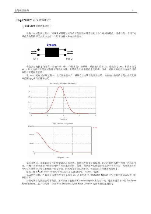
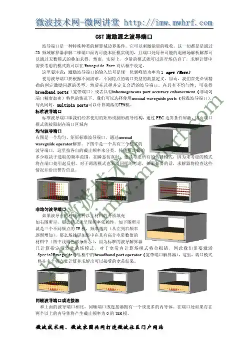
Faq-020802: 定义激励信号1) CST MWS自带的激励信号在整个时域仿真过程中，时域求解器通过时间信号的激励来计算空间上各个时刻的场值。

因此任何一个用于时域仿真的结构都至少应该含有一个用于场输入和输出的端口。

将仿真结构抽象为含有一个输入端口和一个输出端口的系统，根据输入信号i1，输出信号o2,1和反射信号o1,1，以及这些信号的频域值即可得系统特性，并最终设计出需要的系统结构。

因此，时域仿真过程中选择合适的激励信号是很重要的。

在MWS的时域求解过程中，定义激励端口后，系统会给出缺省的激励信号，该缺省的激励信号是由仿真的频率范围决定的高斯脉冲信号。

如上图所示，高斯脉冲信号的频谱仍是高斯函数。

高斯脉冲带宽是有限的，因此可以确保整个频带上网格的生成，有利于求解器在整个频带上对所有频点进行采样。

另外，高斯脉冲的频谱在带宽中不含有零点，故高斯脉冲信号可以在其频带上可以准确地计算S参量。

因此对S参量的求解等，该缺省的高斯脉冲就足够了。

微波工作室®的信号库中含有几个预先定义好的激励信号，可供用户选择。

完成结构建模，并设置好仿真频率等仿真参数后，点击导航树ÖExcitation Signals即可查看当前缺省设置下的激励信号。

如果对缺省的激励信号不满意，还可以在导航树的Excitation Signals上点击右键，选择右键菜单中的Load from Signal Library.....打开信号库（Load New Excitation Signal From Library）选择需要的激励信号。

在下图的信号库对话框中选择需要的激励信号后，点击Apply按钮即可完成信号的加载，在以后的仿真中，可以从求解器对话框中加载该信号对结构进行激励。

2) 自定义激励信号如果信号库中的信号都不能符合仿真要求，您还可以自己定义需要的激励信号。

完成结构建模，并设置好仿真频率等仿真参数后，在导航树的Excitation Signals上点击右键选择右键菜单中的New Excitation Signal......在打开的Excitation Signal对话框中选择Gaussian选项即可通过设定频率范围Fmin和Fmx来定义高斯脉冲信号，选择Rectangular选项即可通过指定信号的上升（Trise）、下降（Tfall）、保持（Thold）以及总激励时间（Ttotal）来定义矩形脉冲信号，并可以在Name栏中为定义的激励信号指定一个您喜欢的名字，这里我们定义一个矩形脉冲，并将名字命名为rectangular。

CST (Computer Simulation Technology) 是一款电磁场仿真软件，可以用来模拟电磁波在各种材料和结构中的传播和散射特性。

如果您想要使用 CST 编写方波信号，可以通过以下步骤来实现：
1. 打开 CST 软件，并创建一个新的项目。

2. 在项目窗口中，选择“Signal”选项卡，并创建一个新的信号。

3. 在信号编辑器中，选择“Analog”选项卡，并设置信号的频率、幅度和相位等参数。

4. 将信号设置为方波信号，可以通过设置信号的上升沿和下降沿时间来实现。

5. 在 CST 中创建一个新的电磁波源，并将方波信号连接到该源。

6. 运行仿真，并观察电磁波在材料和结构中的传播和散射特性。

需要注意的是，CST 是一款专业的电磁场仿真软件，需要一定的专业知识和技能才能熟练使用。

如果您不熟悉 CST 的使用方法，建议先学习 CST 的基本操作和原理，再尝试编写方波信号。

CST宏讲解Examples OverviewThe usage of the VBA macro language is described in detail in the printed documentation "Advanced topics".Here are some typical examples to get in touch with the CST MICROWAVESTUDIO® VBA language:GeneralHow to use the VBA Objects in general.Modelling:Create analytical 2D curve.Create analytical 3D curve.Solver and Post processingAccessing S-Parameter Phase.Calculating the real part of S11 at a certain frequency.Define an excitation function.Adding user defined entries to the result tree.Creating 3D scalar and vector plots:Create a farfield array.How to use the VBA ObjectsExample 1: Call CST MICROWAVE STUDIO? from within an external application Creates a CST MICROWAVE STUDIO? Application Object, opens a project and creates a brick: dim app as Object‘Starts the CST MICROWAVE STUDIO?set app = CreateObject(”MWStudio.Application”)app.OpenFile(”c:Exampleswg.mod”)dim br as Objectset br = CreateObj ect(”MWStudio.Brick”)With br.Reset.Name "BrickOne".Layer "default".Xrange "0", "1".Yrange "0", "2".Zrange "0", "4".CreateEnd WithExample2: Open a file within the build-in VBA interpreterOpens a project from the VBA-Interpreter of the CST MICROWA VE STUDIO?: OpenFile(”c:Exampleswg.mod”) With br.Reset.Name "BrickOne".Layer "default".Xrange "0", "1".Yrange "0", "2".Zrange "0", "4".CreateEnd WithCreate an anayltical 2D curve'--------------------------------------------------' arbitrary xy-function is converted into a curve'--------------------------------------------------Sub Main ()On Error GoTo Curve_ExistsCurve.NewCurve "2D-Analytical"Curve_Exists:On Error GoTo 0Dim sCurveName As StringBeginHideDim iii As Integeriii = 1While SelectTreeItem("Curves2D-Analyticalspline_"+CStr(iii)) iii = iii+1WendsCurveName = "spline_"+CStr(iii)assign "sCurveName"EndHideWith Spline.Reset.Name sCurveName.Curve "2D-Analytical"' ====================================== ' Do not change ABOVE this line' ====================================== ' -----------------------------------------------------------' adjust x-range as for-loop parameters (xmin,max,stepsize) ' enter y-Function-statement within for-loop' fixed parameters a,b,c have to be declared via Dim-Statement' -----------------------------------------------------------' NOTE: available MWS-Parameters can be used without' declaration at any place (loop-dimensions, ...)' (for parametric curves during parameter-sweeps and optimisation !) ' ------------------------------------------- Dim xxx As Double, yyy As DoubleDim aaa As Double ' not necessary if aaa is model parameter aaa = 1.23456/Atn(0.5)For xxx = 1.5 To 10 STEP 0.5yyy = 3*aaa/xxx + Sin(xxx^2).LineT o xxx , yyyNext xxx' ====================================== ' Do not change BELOW this line' ====================================== .CreateEnd WithSelectTreeItem("Curves2D-Analytical"+sCurveName)End SubCreate an analytical 3D curve'--------------------------------------------------' arbitrary analytical xyz-function is converted into a curve '--------------------------------------------------Sub Main ()On Error GoTo Curve_ExistsCurve.NewCurve "3D-Analytical"Curve_Exists:On Error GoTo 0Dim sCurveName As StringBeginHideDim iii As Integeriii = 1While SelectTreeItem("Curves3D-Analytical3dpolygon_"+CStr(iii))iii = iii+1WendsCurveName = "3dpolygon_"+CStr(iii)assign "sCurveName"With Polygon3D.Reset.Name sCurveName.Curve "3D-Analytical"' ====================================== ' Do not change ABOVE this line' ====================================== ' -----------------------------------------------------------' adjust x-range as for-loop parameters (xmin,max,step)' enter y/z-Function-statement within for-loop' fixed parameters a,b,c have to be declared via Dim-Statement' -----------------------------------------------------------' NOTE: available MWS-Parameters can be used without' declaration at any place (loop-dimensions, ...)' (for parametric curves during parameter-sweeps and optimisation !)' -------------------------------------------Dim xxx As Double, yyy As Double, zzz As DoubleDim aaa As Double ' not necessary if aaa is model parameter aaa = 0.3For xxx = Pi/2 To 10*2*Pi STEP 0.2yyy = Sqr(2*Abs(Cos(xxx))) + 3*aaa/xxx + 2*Sin(xxx)zzz = Abs(yyy) - Sqr(2*Abs(Cos(xxx))) + 3*aaa/xxx + 2*Sin(xxx) .Point Sin(xxx) , Cos(xxx) , aaa*xxxNext xxx' ====================================== ' Do not change BELOW this line' ======================================End WithSelectTreeItem("Curves3D-Analytical"+sCurveName)End SubAccessing S-Parameter PhaseExample 1: Accessing all values of S-Parameter phase, stored in file ^p1(1)1(1).sig With Result1D ("p1(1)1(1)") ‘ Co nnect to phase of S11nn = .GetN ‘ Get number of frq-pointsFor ii = 0 To nn-1' Read all points; index of first point is zero.v x = .GetX(ii) ‘ here: frequencyvy = .GetY(ii) ‘ here: according phaseNext iiEnd WithCalculating the real part of S11 at a certain frequencyCalculating the real part of S11 at a certain frequency (here 0.65 GHz)Dim a11 As ObjectDim p11 As ObjectSet a11 = Result1D ("a1(1)1(1)")Set p11 = Result1D ("p1(1)1(1)")Dim n As IntegerDim frq As Doublefrq=0.65n=a11.GetClosestIndexFromX(frq)phase = Pi/180.0 * p11.GetY(n)ampli = a11.GetY(n)real = ampli * cos(phase)ResultTree ExamplesThe ResultTree VBA Object offers very interesting possibilities to configure the Navigation Tree. It is possible to insert different simulation results as well as VBA macros. The following examples will show its functionality.Examples to add Signal Views into the treeAll following examples add items into the folder ”My S-Parameters”. If this folder does not exist it will be crea ted.For inserting signals into the tree it is possible to import results from other projects. Therefore the complete result file name must be specified with the File method. If the results of the current project shall be inserted, the project name in the result file name may be omitted.Signal into Tree 1: Adds a linear view of the amplitude of an extern S11 S-Parameter into the folder.Signal into Tree 2: Adds a linear view of the phase of an extern S11 S-Parameter into the folder.Signal into Tree 3: Adds a Smith Chart view of a S11 S-Parameter into the folder.Signal into Tree 4: Adds a Polar Plot of the S11 S-Parameter into the folder.Examples to add Field Plot Views into the treeFor results others than Signals only those of the current project can be inserted into the tree!Field Plot into Tree: Adds a 3D-Vector plot into the tree.Farfield into Tree: Adds a Farfield into the tree.Examples to add a macro into the treeEvery time a macro is executed from the tree, a VBA command interpreter is started and evaluates the string that has been set by the Macro method. Therefore no variables that are defined within the script that creates the folder entry can beaccessed by the macro. Macro into Tree 1: Adds a command to start the time domain solver into the tree.Macro into Tree 2: Adds a macro into the tree.Macro into Tree 3: Adds an external VBA script into the tree.Signal into Tree 1Adds a linear view of the amplitude of the S11 S-Parameter from the projectxtProj?into the folder. ExtProj is supposed to be located in the directory of the current project.With ResultTree.Reset.Name "My S-ParametersS11 (lin)" ' The entry name and its destination folder.Title "S11 (linear)" ' Title of the plot.File "ExtProj^a1(1)1(1).sig" ' The name of the signal file.Type "XYSignal" ' Plot Type.XLabel "f/Hz" ' Label for the x-axis.Subtype "Linear" ' Sub Plot Type.AddEnd WithSee also: Result TreeSignal into Tree 2Adds a linear view of the phase of the S11 S-Parameter from the project ?xtProj?into the folder. ExtProj is supposed to be located in the directory of the current project.With ResultTree.Reset' The entry name and its destination folder.Name "My S-ParametersS11 (phase)".Title "S11 (phase)" ' Title of the plot.File "ExtProj^p1(1)1(1).sig" ' The name of the signal file.Type "XYSignal" ' Plot Type.XLabel "f/Hz" ' Label for the x-axis.Subtype "Phase" ' Sub Plot Type.AddEnd WithSee also: Result TreeSignal into Tree 3Adds a Smith Chart view of the S11 S-Parameter from the current project into the folder.A value has to be given to which the values in the plot are normalized.With ResultTree.Reset' The entry name and its destination folder.Name "My S-ParametersS11 (Smith Chart)".Title "S11" ' Title of the plot.ReferenceImpedance "50" ' Impedance to which the Values ' will be normalized' Result files with the amplitude and phase values.File "^a1(1)1(1).sig".File2 "^p1(1)1(1).sig".Type "SmithSignal" ' Type of the plot.AddEnd WithSee also: Result TreeSignal into Tree 4Adds a Polar Plot view of the S11 S-Parameter from the current project into the folder. With ResultTree.Reset' The entry name and its destination folder.Name "My S-ParametersS11 (polar)"' Result files with the amplitude and phase values.File "^a1(1)1(1).sig".File2 "^p1(1)1(1).sig".Type "PolarSignal" ' Type of the plot.AddEnd WithField Plot into TreeAdds a Field Plot view of the electric field from the current project into the folder ”MyFieldView”.With ResultTree' The entry name and its destination folder.Name "My FieldViewE_Field".File "^e1_1.m3d" ' Result file name.Type "Efield3D" ' Entry type.AddEnd WithFarfield into TreeAdds a Farfield Plot view from the current project into the folder ?y FieldView?With ResultTree' The entry name and its destination folder.Name "My FieldViewFarfield".File "^ff1_1.ffm" ' Result file name.Type "Farfield" ' Entry type.AddEnd WithMacro into Tree 1Adds a command into the ?serdefined?folder that starts the time domain solver.With ResultTree' The entry name and its destination folder.Name "UserdefinedMacro1"' String to be evaluated by the VBA Interpreter.Macro "Solver.Start".Type "Macro" ' Entry type.AddEnd WithMacro into Tree 2Adds the pr eviously defined control macro ”AutoTest” into the tree.At first a string will be defined that contains a VBA command that executes the control macro. The command is ”RunMacro” that takes a string (the name of the control macro) as its argument. However, strings have to be specified within quotes. Unfortunately quotes are special characters which are not recognized as normal characters. They mark the start and the end of a string. Therefore the variable a is defined with a single quote as its only content. With this quote the entire command string can be constructed.Dim a As Stringa = """a = "RunMacro " & a & "AutoTest" & a' a contains the string: RunMacro "AutoTest"With ResultTree' The entry name and its destination folder.Name "UserdefinedMacro2"' String to be evaluated by the VBA Interpreter.Macro a.Type "Macro" ' Entry type.AddEnd WithMacro into Tree 3Adds an external VBA script into the tree. Let the name of the external macrobe ”Macro1.bas” that will be located in the directory of t he current project.At first a string will be defined that contains a VBA command that executes an external VBA script file. The command is ”MacroRun” that takes a string (the name of t he script) as its argument. However, strings have to be specified within quotes. Unfortunately quotes are special characters which are not recognized as normal characters. They mark the start and the end of a string. Therefore the variable a is defined with a single quote as its only content. With this quote the entire command string can be constructed.Dim a As Stringa = """a = "MacroRun " & a & "Macro1.bas" & a' a contains the string: MacroRun "Macro1.bas"With ResultTree' The entry name and its destination folder.Name "UserdefinedMacro3"' String to be evaluated by the VBA Interpreter.Macro a.Type "Macro" ' Entry type.AddEnd WithScalarPlot3D ExampleThe following script plots surfaces of equal amplitude of the vector field component Y of the electric field ”e1”.‘ Plot only a wire frame of the structure to be able to look insidePlot.wireframe True‘ Select the Y-Component of the electric field e1 in the tree SelectTreeItem ("2D/3D ResultsE-Fielde1Y")‘ Plot the scalar field of the selecte d monitorWith ScalarPlot3D.Type "isosurfaces".PlotAmplitude False.Scaling 50.LogScale False.ContourLines False.ScaleToVectorMaximum True.Quality 60.PlotEnd WithSee Also: SelectTreeItem, PlotVectorPlot3D ExampleThe following script plots the electric field ”e1” (if available) in a linear scale by using 400 colored arrows.‘ Plot only a wire frame of the structure to be able to look insidePlot.wireframe True‘ Select the desired monitor in the tree.SelectTreeItem ("2D/3D ResultsE-Fielde1")‘ Plot the field of the selected monitorWith VectorPlot3D.Type "arrowscolor".Objects 400.Scaling 50.LogScale False.PlotEnd WithSee Also: SelectTreeItem, PlotFarfieldArray ObjectGroup: PostprocessingDescription: Defines the antenna array pattern for a farfieldplot based on a single antenna element.Methods: Reset , UseArray , Arraytype , XSet , YSet , Zset , SetList , DeleteList , AntennaFunctions: noneExample:With FarfieldArray.Reset.UseArray "True".Arraytype "Rectangular".ZSet "2", "2,5", "90".SetList.Arraytype "Edit".Antenna "0", "0", "0", "1.0", "0"End With。

VBA程序设计基础教程VBA（Visual Basic for Applications）是一种宏编程语言，广泛应用于Microsoft Office套件中的各种应用程序，如Excel、Word和Access等。

它能够帮助用户自动化任务、增加功能、提高效率等。

本文将介绍VBA程序设计的基础知识和技巧。

接下来，需要了解VBA的基本语法和语句。

VBA使用类似于其他编程语言的语法，包括变量的声明、条件和循环语句等。

可以使用Dim语句声明变量，例如Dim x As Integer。

可以使用If语句进行条件判断，例如If x > 10 Then...End If。

可以使用For循环语句进行迭代，例如For i = 1 to 10...Next i。

在VBA中，可以使用对象模型来操作应用程序中的对象。

每个Office应用程序都有自己的对象模型，其中包含了各种对象和属性、方法。

通过这些对象和属性、方法，可以对应用程序进行自定义和控制。

例如，在Excel中，可以使用Worksheet对象表示工作表，Range对象表示单元格区域，可以使用Range对象的Value属性获取或设置单元格的值。

VBA还提供了大量的内置函数，可以用于处理数据和执行各种操作。

这些函数包括数学函数、字符串函数、日期和时间函数等。

例如，可以使用Sum函数计算一列数据的和，可以使用Len函数计算字符串的长度，可以使用Date函数获取当前日期等。

在编写VBA程序时，还需要注意一些最佳实践。

首先，应该对变量进行适当的命名，以反映其用途或内容。

其次，应该合理地使用注释，对代码进行解释和说明。

此外，要按照模块或功能将代码分组，以提高程序的可读性和维护性。

最后，应该经常进行代码测试和调试，以确保程序的正确性和稳定性。

总结起来，VBA程序设计是一项强大而有用的技能，可以帮助用户自动化任务、增加功能和提高效率。

通过学习VBA的基础知识和技巧，可以编写出高效、可靠的程序。

第二章 VBA创建界面VBA采用VB的编程语言和语法，是一种可视化的、面向对象的、采用事件驱动的结构化高级程序设计语言，不过VBA的部分函数与VB的不一样，这一点需要注意。

一个完整的VBA程序通常包含以下几个部分：①界面。

界面也就是人机对话框，用户可以通过输入相关数据、点击操作按钮，让VBA进行各种数据计算、模型创建、数据输出等功能。

②主程序。

主程序也就是Sub Main和End Sub之间的程序，主程序可以实现宏文件的特定功能，是一个完整的程序体。

③子程序。

子程序可以完成某个具体的小功能，是为主程序服务的。

有时候主程序需要反复执行同一操作，若每次都编写同样的程序，则显得过于冗杂。

因此编写功能很小、但很具体的子程序，可以随时调用。

④数据输出。

有的时候，经过计算的数据需要输出到txt文件、打印成报表格式等，因此程序中还应该具备数据输出的功能。

当然，该功能是附属功能，可以不存在。

如果一个宏程序中包含了上述四个部分，那么该宏程序就是一个非常完整、功能齐全的程序了。

接下来首先讲解如何利用VBA创建界面。

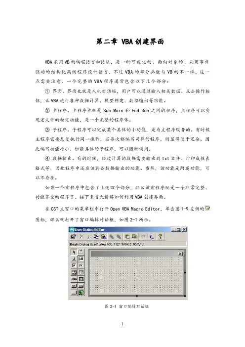
在CST主窗口的菜单栏中打开Open VBA Macro Editor，单击图1-9左侧的图标，那么就打开了窗口编辑对话框，如图2-1所示。

图2-1 窗口编辑对话框之前使用过VB软件的可能会发现，VBA此时的操作界面竟然和VB的操作界面一模一样，都具备可视化的效果。

图2-1左侧部分是窗体中可以使用的控件，包括text文本框、单选按钮等等，中部是放置控件的载体，它的大小可以任意调整，而调整后的大小就是实际的窗体大小。

需要注意的是：创建的窗体中必须至少包含OKButton和CancelButton 中的一个，否则系统会提示存在错误。

2.1 控件① Text静态文本静态文本text通常用来显示数据输出，或者提示用户的标签等。

在窗体中添加一个静态文本，双击便可打开并查看text1静态文本的部分属性，如图2-2所示。