微观经济学讲义(黄有光)

Advanced MicroeconomicsTopic 3: Consumer DemandPrimary Readings: DL – Chapter 5; JR - Chapter 3; Varian, Chapters 7-9.3.1 Marshallian Demand FunctionsLet X be the consumer's consumption set and assume that the X = R m +. For a given price vector p of commodities and the level of income y , the consumer tries to solve the following problem:max u (x )subject to p ⋅x = yx ∈ X• The function x (p , y ) that solves the above problem is called the consumer's demand function .• It is also referred as the Marshallian demand function . Other commonly known namesinclude Walrasian demand correspondence/function , ordinary demand functions , market demand functions , and money income demands .• The binding property of the budget constraint at the optimal solution, i.e., p ⋅x = y , is theWalras’ Law .• It is easy to see that x (p , y ) is homogeneous of degree 0 in p and y .Examples:(1) Cobb-Douglas Utility Function:From the example in the last lecture, the Marshallian demand functions are:where ∑==mi i 1αα. (2) CES Utility Functions:Then the Marshallian demands are:where r = ρ/(ρ -1). And the corresponding indirect utility function is given byLet us derive these results. Note that the indirect utility function is the result of the utility maximization problem:Define the Lagrangian function:The FOCs are:Eliminating λ, we getSo the Marshallian demand functions are:with r = ρ/(ρ-1). So the corresponding indirect utility function is given by:3.2 Optimality Conditions for Consumer’s Problem First-Order ConditionsThe Lagrangian for the utility maximization problem can be written asL = u (x ) - λ( p ⋅x - y ).Then the first-order conditions for an interior solution are:yu i p x u i i =⋅=∇∀=∂∂x p p x x λλ)( i.e. ;)( (1)Rewriting the first set of conditions in (1) leads towhich is a direct generalization of the tangency condition for two-commodity case.Sufficiency of First-Order ConditionsProposition: Suppose that u(x) is continuous and quasiconcave on R m+, and that(p, y) > 0. If u if differentiable at x*, and (x*, λ*) > 0 solves (1), then x* solve the consumer's utility maximization problem at prices p and income y.Proof. We will use the following fact without a proof:•For all x, x'≥0 such that u(x') ≥u(x), if u is quasiconcave and differentiable at x, then ∇u(x)(x' - x) ≥ 0.Now suppose that ∇u(x*) exists and (x*, λ*) > 0 solves (1). Then,∇u(x*) = λ*p,p⋅x* = y.If x* is not utility-maximizing, then must exist some x0≥0 such thatu(x0) > u(x*) and p⋅x0≤y.Since u is continuous and y > 0, the above inequalities implies thatu(t x0) > u(x*) and p⋅(t x0) < yfor some t∈ [0, 1] close enough to one. Letting x' = t x0, we then have∇u(x*)(x' - x) = (λ*p)⋅( x' - x) = λ*( p⋅x' - p⋅x) < λ*(y - y) = 0,which contradicts to the fact presented at the beginning of the proof since u(x1) > u(x*). Remark•Note that the requirement that (x*, λ*) > 0means that the result is true only for interior solutions.Roy's IdentityNote that the indirect utility function is defined as the "value function" of the utility maximization problem. Therefore, we can use the Envelope Theorem to quickly derive the famous Roy's identity.Proposition (Roy's Identity?): If the indirect utility function v(p, y) is differentiable at (p0, y0) and assume that ∂v(p0, y0)/ ∂y≠ 0, thenProof. Let x* = x(p, y) and λ* be the optimal solution associated with the Lagrangian function:L = u(x) - λ( p⋅x - y).First applying the Envelope Theorem, to evaluate ∂v(p0, y0)/ ∂p i givesBut it is clear that λ* = ∂v(p, y)/ ∂y, which immediately leads to the Roy's identity.Exercise•Verify the Roy's identity for CES utility function.Inverse Demand FunctionsSometimes, it is convenient to express price vector in terms of the quantity demanded, which leads to the so-called inverse demand functions.•the inverse demand function may not always exist. But the following conditions will guarantee the existence of p(x):•u is continuous, strictly monotonic and strictly quasiconcave. (In fact, these conditions will imply that the Marshallian demand functions are uniquely defined.)Exercise (Duality of Indirect and Direct Demand Functions):(1) Show that for y = 1 the inverse demand function p = p(x) is given by:(Consult JR, pp.79-80.)(2) Show that for y = 1, the (direct) demand function x = x(p, 1) satisfies(Hint: Use Roy’s identity and the homogeneity of degree zero of the indirect utility function.)3.3 Hicksian Demand FunctionsRecall that the expenditure function e(p, u) is the minimum-value function of the following optimization problem:for all p > 0 and all attainable utility levels.It is clear that e(p, u) is well-defined because for p∈R m++, x∈R m+, p⋅x≥ 0.If the utility function u is continuous and strictly quasiconcave, then the solution to the above problem is unique, so we can denote the solution as the function x h(p, u) ≥0. By definition, it follows thate(p, u) = p⋅x h(p, u).•x h(p, u) is called the compensated demand functions, also commonly known as Hicksian demand functions, named after John Hicks when he first discussed this type of demand functions in 1939.Remarks1.The reason that they are called "compensated" demand function is that we mustimpose an artificial income adjustment when the price of one good is changing whilethe utility level is assumed to be fixed.2.It is important to understand that, in contrast with the Marshallian demands, theHicksian demands are not directly observable.As usual, it should be no longer a surprise that there is a close link between the expenditure function and the Hicksian demands, as summarized in the following result, which is again a direct application of the Envelope Theorem..Proposition (Shephard's Lemma for Consumer): If e(p, u) is differentiable in p at (p0, u0) with p0 > 0, then,Example: CES Utility FunctionsLet us now derive the Hicksian demands and the corresponding expenditure function.min {p1x1 + p2x2}subject toThe Lagrangian function isThen the FOCs are:Eliminating λ, we getFrom these, it is easy to derive the Hicksian demand functions given by: where r = ρ/(ρ-1). And the expenditure function isAlternatively, since we know that the indirect utility function is given by:then by using the identitywe can find the expenditure function, i.e.,3.4 Slutsky EquationRecall that (last lecture) under certain regularity conditions on the utility function, the indirect utility function v (p , y ) and the expenditure function e (p , u ) satisfy the following identities:(a) e (p , v (p , y )) = y .(b) v (p , e (p , u )) = u .Furthermore, we have shown that the demand points corresponding to the optimal solutions of both optimization problems are identical. This result can be expressed into the following interesting identities between Marshallian demands and Hicksian demands:x (p , y ) = x h (p , v (p , y ))x h (p , u ) = x (p , e (p , u ))which hold for all values of p , y and u .The second identity leads to a classic differentiation relation between Hicksian demands and Marshallian demands, known as Slutsky equation.Proposition (Slutsky Equation): If the Marshallian and Hicksian demands are all well-defined and continuously differentiable, then for p > 0, x > 0,where u = v (p , y ).Proof . It follows easily from taking derivative and applying Shephard's Lemma.Substitution and Income Effects• The significance of Slutsky equation is that it decomposes the change caused by a pricechange into two effects: a substitution effect and an income effect .• The substitution effect is the change in compensated demand due to the change inrelative prices, which is the first item in Slutsky equation.• The income effect is the change in demand due to the effective change in incomecaused by the price change, which is the second item in Slutsky equation.• The substitution effect is unobservable, while the income effect is observable.Question: From the above diagram (also know as Hicksian decomposition ), can you see crossing property between a Marshallian demand function and the corresponding Hicksian demand? (Hint: there are two general cases.)Slutsky MatrixSo the Slutsky matrix or theProposition (Substitution Properties). The Slutsky matrix S is symmetric and negative semidefinite.Proof. By Shephard’s Lemma (for consumer), we know thatHence S is symmetric. It is evident that S is the Hessian matrix of the expenditure function e(p, u). Since we know that e(p, u) is concave, so its Hessian matrix must be negative semidefinite. Since the second-order own partial derivatives of a concave function are always nonpositive, this implies that s ii≤ 0, i.e.,which indicates the intuitive property of a demand function: as its own price increases, the quantity demanded will decrease. You are reminded that this is a general property for Hicksian demands.For the Marshallian demands, note that by Slutsky equation,Then for a small change in p i, we will have the following:The first item, capturing the own price effect of the Hicksian demands, is of course nonpositive. The sign of the second item depends on the nature of the good:•Normal good: ∂x i(p, y)/ ∂y > 0.•This leads to a normal Marshallian demand function: it is decreasing in its own price.•Inferior good: ∂x i(p, y)/ ∂y < 0.•When the substitution effect still dominates the income effect, the resulting Marshallian demand is also decreasing in its own price.•When the substitution effect is dominated by the income effect, it will lead to a Giffen good, that is, its demand function is an increasing function of its ownprice.Because of Slutsky equation, the Slutsky matrix (i.e., the substitution matrix) also has the following form that is in terms of Marshallian demand functions.We will get back to the above Slutsky matrix in the next lecture when we discuss the integrability problem.3.5. The Elasticity Relations for Marshallian Demand FunctionsDefinition. Let x(p, y) be the consumer’s Marshallia n demand functions. DefineThen1.ηi is called the income elasticity of demand for good i.2.εij is called the price elasticity of the demand for good i with respect to a price change ingood j. εii is the own-price elasticity of the demand for good i. For i≠j, εij is the cross-price elasticity.3.s i is called the income share spent on good i.The following result summarizes some important relationships among the income shares, income elasticities and the price elasticities.Proposition. Let x(p, y) be the consumer’s Marshallian demand functions. Then1.Engel aggregation:2.Cournot aggregation:Proof. Both identities are derived from the Walras’ Law, namely, the fact that the budget is tight or balanced:y = p⋅x(p, y) for all p and y. (A)To prove Engel aggregation, we differentiate both sides of (A) y:as required.To prove Cournot aggregation, we differentiate both sides of (A) p j:Multiplying both sides by p j/y leads toas required too.3.6 Hicks’ Composite Commodity TheoremAny group of goods & services with no change in relative prices between themselves may be treated as a single composite commodity, with the price of any one of the group used as the price of the composite good and the quantity of the composite good defined as the aggregate value of the whole group divided by this price. Important use in applied economic analysis.Additional ReferencesAfriat, S. (1967) "The Construction of Utility Functions from Expenditure Data," International Economic Review, 8, 67-77.Arrow, K. J. (1951, 1963) Social Choice and Individual Values. 1st Ed., Yale University Press, New Haven, 1951; 2nd Ed., John Wiley & Sons, New York, 1963.Becker, G. S. (1962) "Irrational Behavior and Economic Theory," Journal of Political Economy, 70, 1-13.Cook, P. (1972) "A One-line Proof of the Slutsky Equation," American Economic Review, 42, 139. Deaton, A. and J. Muellbauer (1980) Economics and Consumer Behavior. Cambridge University Press, Cambridge.Debreu, G. (1959) Theory of Value. John Wiley & Sons, New York.Debreu, G. (1960) "Topological Methods in Cardinal Utility Theory," in Mathematical Methods in the Social Sciences, ed. K. J. Arrow and M. D. Intriligator, North Holland, Amsterdam. Diewert, W. E. (1982) "Duality Approaches to Microeconomic Theory," Chapter 12 in Handbook of Mathematical Economics, ed. K. J. Arrow and M. D. Intriligator, North Holland, Amsterdam.Gorman, T. (1953) “Community Preference Fields,” Econometrica, 21, 63-80.Hicks, J. (1946) V alue and Capital. Clarendon Press, Oxford, England.Katzner, D.W. (1970) Static Demand Theory. MacMillan, New York.Marshall, A. (1920) Principle of Economics, 8th Ed. MacMillan, London.McKenzie, L. (1957) “Demand Theory Without a Utility Index," Review of Economic Studies, 24, 183-189.Pollak, R. (1969) "Conditional Demand Functions and Consumption Theory," Quarterly Journal of Economics, 83, 60-78.Roy, R. (1942) De l'utilite. Hermann, Paris.Roy, R. (1947) "La distribution de revenu entre les divers biens," Econometrica, 15, 205-225. Samuelson, P. A. (1938) "A Note on the Pure Theory of Consumer's Behavior," Econometrica, 5, 61-71, 353-354.Samuelson, P. (1947) Foundations of Economic Analysis. Harvard University Press, Cambridge, Massachusetts.Sen, (1970) Collective Choice and Social Welfare. Holden Day, San Francisco.Stigler, G. (1950) "Development of Utility Theory," Journal of Political Economy, 59, parts 1 & 2, pp. 307-327, 373-396.Varian, H. R. (1992) Microeconomic Analysis. Third Edition. W.W. Norton & Company, New York. (Chapters 7, 8 and 9)Wold, H. and L. Jureen (1953) Demand Analysis. John Wiley & Sons, New York.。

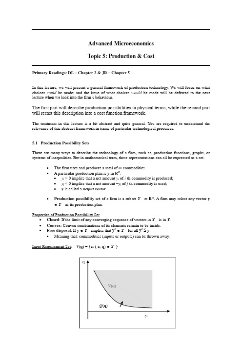
Advanced MicroeconomicsTopic 5: Production & CostPrimary Readings: DL – Chapter 2 & JR – Chapter 5In this lecture, we will present a general framework of production technology. We will focus on what choices could be made; and the issue of what choices would be made will be deferred to the next lecture when we look into the firm’s behaviour.The first part will describe production possibilities in physical terms; while the second part will recast this description into a cost function framework.The treatment in this lecture is a bit abstract and quite general. Y ou are required to understand the relevance of this abstract framework in terms of particular technological processes.5.1 Production Possibility SetsThere are many ways to describe the technology of a firm, such as, production functions, graphs, or systems of inequalities. But in mathematical term, these representations can all be expressed as a set.∙The firm uses and produces a total of m commodities.∙A particular production plan is y in R m:∙y i > 0 implies that a net amount y i of i-th commodity is produced;∙y j < 0 implies that a net amount –y j of j-th commodity is used;∙y is called a netput vector.∙Production possibility set of a firm is a subset Y⊂R m. A firm may select any vector y ∈Y as its production plan.Properties of Production Possibility Set∙Closed: If the limit of any converging sequence of vectors in Y is in Y.∙Convex: Convex combinations of its elements remain to be inside.∙Free disposal: If y∈Y implies that y’∈Y for all y’≤y.∙Meaning that: commodities (inputs or outputs) can be thrown away.Input Requirement Set: V(q) = {z: (-z, q) ∈Y }Isoquant: Q (q ) = {z : (-z , q ) ∈ Y , (-z , q’) ∉ Y ∀ q’ ≥ q , q’ ≠ q }∙ The isoquant Q (q ) is usually the boundary closest to the origin of V (q ).Proposition : If Y is convex, so is V (q ).∙ We normally do not require that the production possibility set is convex. If so, it will ruleout "start-up costs" and other sorts of returns to scale. (Do you see why?)5.2 Production FunctionsTransformation Function of the Production Possibility SetFor most production possibility sets, it is possible to describe them in item of single inequality of the form T (y ) ≤ 0. That is,Y = {y : T (y ) ≤ 0}A function T that describes Y this way is called a transformation function .Efficient Production∙A production point y ∈Y is efficient is there is no y’ ∈Y , y’ ≠ y , with y’ ≥ y .∙ An efficient production implies that it is not possible to either unilaterally increase the output(s)or unilaterally decrease the input(s) while still remaining in Y .Production Functions (Joan Robinson)∙ For those technologies that have a single output can be described by a production function , which has both the theoretical and empirical appeal.∙ The netput vector has the form: (-z , q ), where q is the output.∙If the technology has a transformation function T , i.e., Y = {(-z , q ): T (-z , q ) ≤ 0}, then under certain regularity conditions, we can solve T (-z , q ) = 0 for all q , which leads to another function: q = f (z ). This function f is the production function .∙ The specification of q = f (z ) involves the notion of efficiency since it represents the maximumoutput level that can be achieved with the input, i.e.,f (z ) = max{q’: T (-z , q’) ≤ 0}.∙ With a single output, the input requirement set V (q ) is convex if and only if the corresponding production function f (z ) is a quasiconcave function.MRTS and Separable Production Functions∙ With a given production function q = f (z ), the marginal rate of technical substitution(MRTS) between two inputs i and j is defined as follows:./)(/)()(ji ijz f z f MRTS∂∂∂∂=z z z∙Normally, MRTS ij depends on the specification of all inputs. We can use MRTS to define separableproduction functions , which involves regrouping the inputs into several mutually exclusive and exhaustive subsets. For details, refer to p.221 of Jehle & Reny.Elasticity of SubstitutionsFor a production function f (z ), the elasticity of substitution between inputs i and j at the point z is defined as,))(/)(()(/)(/)/( ))(/)(ln()/ln())(ln()/ln()(z z z z z z z z j i j i ij i j j i i j iji j ij f f d f f z z z z d f f d z z d MRTS d z z d ==≡σwhere f i and f j are the marginal products of inputs i and j , and d (.) is the total differentiation .∙ MRTS is a local measure of substitutability between two inputs in producing a given levelof output. MRTS is not independent of the units of measurement.∙ The elasticity of substitution is defined as the percentage change in the input proportion(z j /z i ) associated with a 1 percent change in the MRTS between the two inputs. The elasticity of substitution is unitless .∙ In general, the closer the elasticity of substitution is to zero, the more difficult substitutionbetween the inputs; the larger it is, the easier substitution between them.CES Production FunctionThe constant elasticity of substitution (CES) production function has the following form:. 0 and 1 where ,)(1i /11i z f q i mi m i i i ∀>=⎪⎭⎫⎝⎛==∑∑==αααρρz∙It can be shown that for the above production function,. 11)(j i ij ≠∀-=ρσzSpecial Cases of CES Production Function∙ Linear Homogeneous Cobb-Douglas Production Function:∙ Correspond to the case when ρ → 0. (σij → 1) ∙ The basic functional form is.)(1∏===mi iizf q αz∙ A proof (for the case of n = 2) is in the Appendix of this note.∙Leontief Production Function:∙ Correspond to the case when ρ → - ∞. (σij → 0) ∙ The functional form isq = f (z ) = min{α1z 1, …, αm z m }.∙ The easiest way of proving this result is to check the corresponding MRTS ij of CESproduction function as ρ → - ∞, which lead to specific isoquants that are unique to Leontief technology.∙ Another function form for the Leontief production function is as follows:}.,,min{)(11mm a z a zf q ==z∙It is clear from the function specification that a Leontief technology uses inputs in fixed proportion, which implies that there is a single fixed formula for production.Returns to Scale∙ A production function f (z ) has the property of (globally)1. Constant returns to scale if f (t z ) = t f (z ) for all t > 1 and all z .2. Increasing returns to scale if f (t z ) > t f (z ) for all t > 1 and all z .3. Decreasing returns to scale if f (t z ) < t f (z ) for all t > 1 and all z .∙ The most natural case of decreasing returns to “scale” is the case where we are unable toreplicate some inputs. In fact, it can always be assumed that decreasing returns to scale is due to the presence of some fixed input .∙ To see this, let f (z ) be a production function with decreasing returns to scale. Suppose that weintroduce another "new input" and measured by z 0. Now define a new production function:F (z 0, z ) = z 0 f (z /z 0).It is easy to see that F exhibits constant returns to scale. In this sense, the original decreasing returns technology f (z ) can be thought as a restriction of the constant returns technology F (z 0, z ) that results from setting z 0 = 1.Elasticity of Scale∙ The elasticity of scale is a local measure of returns to scale. It, defined at a point, specifies theinstantaneous percentage change in output as a result of 1 percent increase in all inputs:)()()ln())(ln(lim)(11z z z z f z f t d t f d mi ii t ∑=→==μ∙ We say that returns to scale are locally constant, increasing, or decreasing when μ(x ) is equal to, greater than, or less than one.Constant Returns to Scale and the Marginal Productivity Theory of DistributionFrom the definition of a homogenous production function, differentiation with respect to k, evaluated at k=1, we have sy = Σx i f i where f i ≡δf/δx i .A production function homogenous of degree s, the marginal product of each factor is homogenous of degree s-1. To show this, differentiate with respect to x i .5.3 The Cost FunctionBasic Settings:∙ output vector: q ∈ R +n ;; input vector: z ∈ R +m ; ∙ input factor price vector: w ∈ R +m ;∙ Recall that for the given output vector q , the input requirement set is defined asV (q ) = {z : (-z , q ) ∈ Y }∙ Cost Function . The cost function of a firm is the functionc (w , q ) = min w ⋅zs.t. z ∈ V (q )defined for all w ≥ 0, q ≥ 0.∙ If there is a single output and the production technology is fully represented by the productionfunction q = f (z ), thenc (w , q ) = min w ⋅zs.t. f (z ) ≥ qIf z (w , q ) solves this minimization problem, thenc (w , q ) = w ⋅z (w , q )∙ The solution z (w , q ) is referred to as the firm's conditional input demand functions (alsoknown as conditional factor demand functions), since it is conditional on the level of output q , which at this point is arbitrary and so may or may not be profit-maximizing. ∙ The inequality constraint can usually be replaced by the equality.Calculus Analysis of Cost MinimizationConsider the following cost-minimizing problem:c (w , q ) = min w ⋅zs.t. f (z ) = qThen the corresponding Lagrange function isL (z , λ) = w ⋅z - λ (f (z ) - q ).,,1, /*)(/*)(*)solution interior some for (FOC *)(2m j i MRTSz f z f w w f w ijji i ==∂∂∂∂=⇒∇=⇒z z z z λwhich leads to the geographical illustration of the cost minimization (tangency condition ) indicated asbelow.isoquant must lie above the isocost line. This, for the case of two inputs, leads to that the bordered Hessian matrix of the Lagrangian,⎪⎪⎪⎭⎫ ⎝⎛--------=⎪⎪⎪⎪⎪⎪⎪⎭⎫ ⎝⎛∂∂∂∂∂∂∂∂∂∂∂∂∂∂∂∂∂∂∂∂∂∂∂∂∂=02122221112112212122222212212212212f f f f f f f f L z L z L z Lz L z z L z L z z L z L λλλλλλλλλH has a negative determinant.Examples:∙ Cost function for the Cobb-Douglas technology : q = K 1/2 L 1/2, where K is the capital (witha unit price of w 1 - rental) and L is the labor (with a unit price of w 2 - wage). Then the corresponding cost function is21212);,(w w q q w w c =∙ For the general Cobb-Douglas production function :.)(1∏===mi iizf q αzThe corresponding cost function is given by:∑∏===⎪⎪⎭⎫ ⎝⎛=mi imi i i i w qq c 1/1/1 with ,),(αααααααw∙Cost function for CES T echnology : q = (az 1ρ + bz 2ρ)1/ρ, by using the first-order Lagrangian conditions, we can derive the cost function given by:).1(1with ,);,(/12121≠-=⎥⎥⎦⎤⎢⎢⎣⎡⎪⎭⎫ ⎝⎛+⎪⎭⎫ ⎝⎛=ρρρr b w a w q q w w c rr r∙Cost function for Leontief T echnology :}.,,min{)(11mm a z a z f q ==zIts cost function is given by: c (w , q ) = q w ⋅a .General Properties of Cost Functions∙ If the production function f is continuous and strictly increasing, then c (w , q ) is1. Zero when q = 0.2. Continuous on its domain3. For any all w > 0, strictly increasing and unbounded above in y .4. Increasing in w .5. Homogenous of degree one in w .6. Concave in w .5.4 Conditional Input Demand FunctionsFor the given cost minimization problem, the solution z (w , q ) is the firm's conditional input demand function. Applying the usual argument, z (w , q ) must satisfy the first-order conditions:.)),((,)),((0w z w w z ≡∇-≡q f q q f λDifferentiating these identities with respect to w we will have the following:w w z w z w z I 0w z w z =∇∇-∇∇-=∇∇)),()),(()),()),(()),()),((2q q f q q f q q f λλwhich, in term of matrices, become:⎪⎪⎭⎫ ⎝⎛-=⎪⎪⎭⎫ ⎝⎛∇∇⎪⎪⎭⎫ ⎝⎛∇-∇-∇-0),(),(0)()()(2I w w z z z z q q f f f T λλ From this, we can solve for the substitution matrix ∇z (w , q ) by taking the inverse of the bordered Hessain matrix:⎪⎪⎭⎫⎝⎛⎪⎪⎭⎫ ⎝⎛∇∇∇=⎪⎪⎭⎫ ⎝⎛∇∇-00)()()(),(),(12I z z z w w z f f f q q Tλλ∙ This result is in fact associated with comparative statics of the conditional input demand functions with respect to the input prices.∙Shephard's Lemma : (The derivative property) Let z (w , q ) be the firm's conditional input demand function. Assume that c (w , q ) is differentiable at w with w > 0, and.,...,1 ),,(),(n i q z w q c i i==∂∂w w∙ This result is a direct application of Envelope Theorem .∙Shephard's lemma implies that the cost function is a non-decreasing function of input prices .Note:∙It is easy to see that the conditional input demand functions are homogeneous of degree 0.5.5 Short-Run & Long-Run CostsRecall that the cost function can be expressed as the value of conditional input demands:c (w , q ) = w ⋅z (w , q ).∙ In short-run, some of the inputs are fixed. Let z f be the vector of fixed inputs, z v the vector ofvariable inputs. We also break the vector of input prices w = (w v , w f ). ∙ The short-run conditional input demand functions: z v (w , q , z f ). ∙ Short-run cost function is then given by:sc (w , q , z f ) = w v z v (w , q , z f ) + w f z f ≡ SVC + FC = STC∙ Other derived cost concepts are∙ Short-run average cost (SAC) = s c (w , q , z f )/q ∙ Short-run average variable cost (SA VC) = SVC/q ∙ Short-run average fixed cost (SAFC) = FC/q ∙ Short-run marginal cost (SMC) = ∂s c (w , q , z f )/∂q∙ In the long-run, all production factors are variable. In this case, the firm must optimize in thechoice of z f . We can express the long-run cost function in terms of the short-run cost function in the following way.∙ Let z f (w , q ) be the optimal choice of the fixed inputs, and let z v (w , q ) = z v (w , q , z f (w , q )).Then the long-run cost function is given by:c (w , q ) = w v z v (w , q ) + w f z f (w , q ) = sc (w , q , z f (w , q )).∙ Similarly, we will have two derived long-run cost concepts:∙ Long-run average cost (LAC) = c (w , q )/q ∙ Long-run marginal cost (LMC) = ∂c (w , q )/∂qProposition (Cost Envelope) - Relationship Between Short-run & Long-Run CostsFor ease of presentation, we drop the argument of w (the fixed input prices) assume a single fix input z . Then, c (q ) = sc (q , z (q )).∙ For a given output q*, let z* = z (q*) is the associated (optimal) long-run demand for the fixed input.Then it is clear that∙ The short-run cost, sc(q, z *), must be least as large as the long-run cost, c (q , z (q )), for alllevels of output.∙ The short-run cost will equal to the long-run cost at the output q = q *, i.e.,sc (q *, z *) = sc (q *, z (q *)) = c (q *).This implies that the long-run and the short-run cost curves must be tangent at q *.∙ The above result follows from the following argument, which comes from the envelopetheorem:,*)*,(*)(*)*,(*)*,(*)(*,(*)(qz q sc dq q dz z z q sc q z q sc dq q z q dsc dq q dc ∂∂=∂∂+∂∂== since z * is the optimal choice of the fixed input at the output level q *, which implies that.0*)*,(=∂∂zz q sc∙ Finally, note that if the long-run and short-run cost curves are tangent, the long-run and short-run average cost curves must also be tangent. In other word, the long-run average cost curve is the lower envelope of the short-run cost curves. ∙The geometric illustration of the above result is as follows:T echnical Appendix of T opic 5Derivation of Cobb-Douglas Production Function from CES FormIt suffices to consider the case for n = 2. Note that()ρυραα/12121)1(),(z z z z f q -+==We need to work out the limit of f as ρ → 0. Since (α (z 1)ρ + (1- α) (z 2)ρ ) → 1 as ρ → 0, the limitingproblem of f as ρ → 0 becomes an indeterminate form of 0∞. To find the limit of this nature, we have to find the limit of the logarithm of f :]ln[))(ln 1()(ln 1])1([]))(ln 1()(ln [lim))1(ln(lim),(ln lim 121212122110210210ααρρρρρρρρρααααααραα-→→→⨯=-+=-+-+=-+=z z z z z z z z z z z z z z f(Here we have used two results from Calculus: (1) the formula for the derivative of a x: d(a x)/d x = (lna )(a x); and (2) L'Hopital's Rule.) Therefore, we have.),(lim 121210ααρ-→=z z z z fFor the general case, the proof is similar.Additional References:Arrow, K. J., H. Chenery, B. Minhas, and R. M. Solow (1961) "Capital-Labor Substitution andEconomic Efficiency," The Review of Economics and Statistics , vol. 43, 225-250.Blackorby, C. and R. R. Russell (1989) "Will the Real Elasticity of Substitution Please Stand Up? (AComparison of the Allen/Uzawa and Morishima Elasticities)," American Economic Review , vol. 79, 882-888.Diewert, W. E. (1971) "An Application of the Shephard Duality Theorem: A Generalized LeontiefProduction Function," Journal of Political Economy , vol. 79, 481-507.Diewert, W. E. (1975) “Applications of Duality Theory,” in Frontiers of Quantitative Economics , ed. M.D. Intriligator and D. A. Kendricks, North Holland, Amsterdam.Diewert, W. E. (1982) “Duality Approaches to Microeconomic Theory ,” in Handbook ofMathematical Economics , vol. 2, ed. K. J. Arrow and M. D. Intriligator, North Holland, Amsterdam.Nadiri. M. I. (1982) “Producer’s Theory,” in Handbook of Mathematical Economics , vol. 2, ed. K. J.Arrow and M. D. Intriligator, North Holland, Amsterdam.Shephard, R. W. (1970) Theory of Cost and Production Functions . Princeton: Princeton UniversityPress.Uzawa, H. (1962) "Production Functions with Constant Elasticities of Substitution," The Review ofEconomic Studies , vol. 29, 291-299.。

ECC5650- Microeconomic TheoryTopic 7MesoeconomicsA Micro- Macroeconomic AnalysisThis topic provides a micro-macroeconomic analysis with elements of general equilibrium without assuming perfect competition. It concentrates on a representative firm, taking account of the influence of macro variables like the price level, aggregate income/output, and interactions with the rest of the economy. It is called mesoeconomics as it synthesizes micro, macro and general equilibrium analysis. It provides many comparative-static results, including the Keynesian and the Monetarist results on the effects of a change of nominal aggregate demand as special cases.ReferencesY ew-Kwang Ng, “A micro-macroeconomics analysis based on a representative firm”, Econmica, 1982, 49: 121-139.Y.-K. Ng, Mesoeconomics: A Micro-Macro Analysis, London: Harvester, 1986.Ng, “Business confidence and depression prevention: A mesoeconomic perspective”, American Economic Review, 1992, 82(2): 365-371.Ng, “Non-neutrality of money under non-perfect competition: why do economists fail to see the possibility?” In Arrow, Ng, and Y ang, eds., Increasing Returns and Economic Analysis, London: Macmillan, 1998, pp.232-252.Ng, “On estimating the effects of events like the Asian financial crisis: A mesoeconomic approach”, Taiwan Economic Review（經濟論文叢刊）, 27 (4): 393-412, December 1999.Mesoeconomic Analysis(A4) q xF p p g gi i Ig N I≡==∑111(,...,,,...,)ααTwo simplifications: 1. used by virtually all macro and aggregative studies of ignoring distributional effects by replacing the vector α1, ..., αI by α ≡ ∑αi .2. concentrate on the representative firm and replace the price vector of all other firms by theIn Ng (1986, Appendix 3I), a fully general equilibrium analysis is used to show that (1) for any (exogenous) change (in cost or demand) there exists (in a hypothetical sense) a representative firm whose response to the change accurately (no approximation needed) represents the response of the whole economy in aggregateoutput and average price, and (2) a representative firm defined by a simple method (that of a weighted average) can be used as a good approximation of the response of the whole economy to any economy-wide change in demand and/or costs that does not result in drastic inter-firm changes. The representative firm takes the aggregate variables as given and maximize its profit:where C = total cost, Y = aggregate output of the economy , εexogenous factors affect costs. The possible effects of Y on C may work through the input market. It may be noted that the cost function is rather general. First-order condition:where ()q C/ c p/q,p q/ ∂∂≡∂∂≡η and μ is marginal revenue. From the representativeness of the firm and the requirement of equilibrium, we havewhere A = real aggregate demand, N = number of firms.The nominal aggregate demand of the economy:where the restriction 1>>0Y αη is similar to the case of the Keynesian cross diagram that the slope of C + I is positive but less than one to avoid an explosive system. Similarly for ηαP . (A11) is a very general function and include the simple Keynesian and Monetarist aggregate demand functions as special cases.Comparative-statics analysis. The total differentiation of (A8), after substituting in the totalwhere xyx y y x, DA A p, P = -p A Aημμηηη≡∂∂≡∂∂∂∂ is the proportionate effect of realaggregate demand on marginal revenue at given prices through possible effects on the demand elasticity (in Ng 1982, D is assumed zero for simplicity), d c c d cc≡∂∂⎛⎝⎫⎭⎪εε is the exogenous change in marginal cost. The total differentiation of (A11), after dividing through by α and substituting in d α/α = dP/P + dY/Y from the total differentiation of (A10), gives where d d ααεεαα≡∂∂⎛⎝ ⎫⎭⎪is the exogenous change in nominal aggregate demand.Substituting dY/Y and dP/P from (A13) in turn into (A12):where ()()()()∆ 1-1-+1-+-D Y cP P cq cY ≡ααηηηηη, ηab ≡ (∂a/∂b)b/a.The effects on the price level and aggregate output depends on the exogenous changes in demand and costs as well as the endogenous response variables, including the slope of the MC curve (of the representative firm), how much MC responds to aggregate output and the price level (shifts in the MC curve), how much the price elasticity of demand changes in response to real aggregate demand, how much the nominal aggregate demand changes in response to realaggregate income and the price level. An estimate of these changes and responses would then give us our estimate of the effects on the price level and aggregate output using the above equations.The effects of an exogenous cost changesThe effects of an exogenous demand changes:The various possible cases: monetarist (traditional), Keynesian, intermediate, expectation wonderland, cumulative expansion/contradiction.Continuum of EquilibriaInterfirm macroeconomic externality⎥⎦⎤⎢⎣⎡-⎪⎪⎭⎫⎝⎛--+-=CY Y CP P ji N q R ηηηηηη∂∂αα1111The effects of the Sep. 11 incident on the economy1. Aggregate demand decreases exogenously; costs increases exogenously . Hence, dY < 0.2. dP ambiguous; opposing effects.3. Expectation wonderland.Long run : where the number of firms is allowed to change, we allow N, the number of firms, to enter the demand function and also add the additional condition of zero long-run profit (A14) ()()pf p /P, /P - C q,Y, P, c αε= 0 Comparative results for the long run: (A15)∇=++-++-++-dP P M E M D E d E dC C M dc c cYcqCYYcqY/[()()](/)()()(/)()(/)ηηηααηηηαα11(A16)∇=-++---+--dY Y M E d E dC C M dc c cPcqCPPcqP/[()()()](/)()()(/)()(/)1111ηηηααηηηααwhere∇=-++-++--++-()[()()](/)()[()()()]1111ηηηηααηηηηααPcYcqCYYcPcqcPM E M D E d M EM ≡ (p-c)/p is the markup of price over marginal cost, E ≡ (∂μ/∂N)N/μ at given prices (where μ ≡ marginal revenue of the representative firm) is the effect on MR of entry of new firms through a higher absolute price elasticity of demand due to increased competition. The long-run effects of a shock may then be analyzed using (A15) and (A16) above by estimating the long-run exogenous changes in aggregate demand and costs as well as the long-run endogenous response variables contained in these two equations.Effects of the incident: Similar to short run in qualitative conclusions but with thedeterminants of the quantitaive effects different.Some Extensions:1.Revenue maximization and AC-pricing (ch.6), making the non-traditional results morelikely.2.Oligopoly (ch.7) –reconciling the apparent inconsistency between the price rigiditypredicted by the kinked demand curve hypothesis with Stigler’s empirical evidence.3.The government sector (ch.10), with the results of a negative balance-budget multiplierand the possibilities of non-inflationary expansion, non-deflationary contraction, self-financing tax reduction.4.The role of the labour market and union power (ch.13); the mistake of increasing wagerates as an anti-depression policy (ch.10).The case of an industry. Ch.5, taxes and cost increases passed on to consumers more than 100%.Also partly explains:1.Why markup pricing is prevalent (ch.8).2.Why business cycles exist (ch.12).3.Why do financial crises matter.4.Why the World Bank and IMF differ in their financial-crisis rescue policies.5.Some controversies in macroeconomics, including the natural rate of unemployment,the non-vertical long-run Phillips curve.6.Why economic forecasts are difficult.。

Department of EconomicsA DVANCED M ICROECONOMICS -Course Outline and Reading Guide Students who have solid background and are not adverse to a mathematical approach may use H.R. Varian, Microeconomic Analysis, Norton, 3rd edition, 1992. An alternative advanced text emphasizing game theory is David M. Kreps, A Course in Microeconomic Theory, Princeton University Press, 1990. Even more advanced texts includes:Andreu Mas-Colell, Michael D. Whinston and Jerry R. Green, 1995. Microeconomics Theory. Oxford University Press. (An advanced textbook in microeconomics theory.)However, the following texts are referred to frequently.Geoffery A. Jehle & Philip J. Reny (2001). Advanced Microeconomic Theory (2nd Edition). Boston: Addison-Wesley. (JR)Y.-K. Ng, Mesoeconomics: A Micro-Macro Analysis, London: Harvester, 1986.A simpler alternative to JR is:David G. Luenberger (1995). Microeconomic Theory. McGraw-Hill. (DL)The following topics are provided for reading. The lectures may not cover all topics and may not proceed in the same order.:(0) Mathematical Introduction (May be skipped if students are already familiar)JR: Ch. A1 & A2DL: Appendix C(1) Basic Consumer TheoryMainly on consumer preferences and the existence of utility functions, properties of demand functions, the composite commodity theorem, and the Slutsky equation.DL: Ch. 4JR: Ch. 1, 2, 3.Ng, Welfare Economics, App.1B.H.A.J. Green, Consumer Theory, Chapters 1-7P.R.G. Layard and A.A. Walters, Microeconomic Theory, McGraw-Hill, Sections 5.1 and 5.2Varian, Chapters 7-9(2) Some ExtensionsR.H. Frank, “If Homo Economicus could choose his own utility function, would he want one with a conscience?” American Economic Review, September 1987,593-604; June 1989, 588-596.Y.-K. Ng, “Step-optimization, secondary constraints, and Giffen goods”, Canadian Journal of Economics, November 1972, 553-560.Y.-K. Ng, “Diamonds are a government’s best friend: Burden-free taxes on goods valued for their values”, American Economic Review, March 1987, 77: 186-191.Y.-K. Ng, “Mixed diamond goods and anomalies in consumer theory: Upward-sloping compensated demand curves with unchanged diamondness”, Mathematical Social Sciences, 1993, 25: 287-293.(3) UncertaintyDL: Ch.11Gravelle & Rees, Chapters 19 and 20Green, Chapters 13, 14 & 15Y.-K. Ng, “Why do people buy lottery tickets? Choices involving risk and the indivisibility of expenditure”, Journal of Political Economy, October 1965, 530-535.Varian, Chapter 11Y.-K. Ng, “Expected subjective utility: Is the Neumann-Morgenstern utility the same as the neoclassical’s?” Social Choice Welfare, 1984, pp. 177-186.(4) Production and Marginal Productivity TheoriesDL: Ch. 5JR: Ch. 2, 3.Baumol, Chapter 11Henderson & Quandt, Chapter 3Varian, Chapters 1-5R.H. Frank, “Are workers paid their marginal products”, American Economic Review, 1984, 549-571.L. Borghans & L. Groot, “Superstardom and monopolistic power: Why media stars earn more than their marginal contribution to welfar e”, Journal of Institutional and Theoretical Economics, 1998, pp.546-(5) Introduction to Mesoeconomic AnalysisY.-K. Ng, Mesoeconomics: A Micro-Macro Analysis, London: Harvester, 1986.Y.-K. Ng, “Business confidence and depression prevention: A meso economic perspective”, American Economic Review, May 1992, 82(2): 365-371.Ng, “Non-neutrality of money under non-perfect competition: why do economists fail to see the possibility?” In Arrow, Ng, and Yang, eds., Increasing Returns and Economic Analysis, London: Macmillan, 1998, pp.232-252.(6) General EquilibriumDL: Ch. 7; JR: Ch.5K.J. Arrow & F. Hahn (1971), General Competitive Analysis, Chapter 1F. Black (1995), Exploring General Equilibrium, Cambridge, Mass.: MIT Press.J.S. Chipman, “The nature and meaning of equilibrium in economic theory”, in D.Martindale, ed., Functionalism in Social Sciences; reprinted in H. Townsend, ed., Price Theory, Penguin.Gravelle & Rees, Chapter 16W. Nicholson, Appendix B to Chapter 19, “The existence of genera l equilibrium prices”, Microeconomic Theory, 1985, The Dryden Press, 684-694.Starr. R.M. (1997). General Equilibrium Theory: An Introduction. Cambridge University Press.Varian, Chapters 17 & 21S. Zamagni, Microeconomic Theory. Oxford: Blackwell, 1987, Ch. 16.(7) Selected Topics in Microeconomic Analysis(a)Adverse selection, signalling, and screening.Akerlof, G. “The market for lemons: quality uncertainty and the market mechanism”, Quarterly Journal of Economics, 1970, 89: 488-500.Mas-Colell, Andreu, Whinston, Michael D. & Green, Jerry R., Microeconomic theory New York : Oxford University Press, 1995, Ch. 13.(b)The principal-agent problemHolmstrom, B., (1979), “Moral hazard and Observability”, Bell Journal of Economics, 10(1), 74-91Mas-Colell, Andreu, Whinston, Michael D. & Green, Jerry R., Microeconomic theory New York : Oxford University Press, 1995, Ch. 14.3typescript.(h) Specialization and Economic OrganizationYang, Xiaokai, Economics: New Classical versus Neoclassical Frameworks, Blackwell, 2001, Chs.5-7, 11.Yang, Xiaokai & Ng, Y.-K. Specialization and Economic Organization: A New Classical Microeconomic Framework. In "Contributions to Economic Analysis", V ol. 215, 1993, Amsterdam: North Holland, pp. xvi + 507. (Mainly Chs.0-2, 5.)Yang, X iaokai & Ng, Siang, “Specialization and Division of Labour: A Survey”, in Kenneth J. Arrow, et al, eds., Increasing Returns and Economic Analysis, London: Macmillan, 1998, pp. 3-63.Yang, Xiaokai & Ng, Y.-K. “Theory of the Firm and Structur e of Residual Rights”, Journal of Economic Behaviour and Organization, V ol. 16, pp. 107-28, 1995.(i)Does the enrichment of a sector benefit others?Ng, "The Enrichment of a Sector (Individual/Region/Country) Benefits Others: The Third Welfare Theorem?", Pacific Economic Review, Nov. 1996, V ol. 1, No.2, pp.93-115.Ng, Siang & Y.-K., “The enrichment of a sector(individual/region/country) benefits others: a generalization”, Pacific Economic Review, Oct. 2000, 5(3): 299-302.Ng, Siang & Y.-K., “The enrichmen t of a sector(individual/region/country) benefits others: the case of trade for specialization”, International Journal of Development Planning Literature, 1999, 14(3): 403-410.。

Overview of the inframarginal analysisWhy economists shifted their attention from the economic organization problem to the resources allocation problem?1)David Ricardo's concept of comparative advantage∙Exogenous comparative advantage∙Endogenous comparative advantage:Smith’s concept of economies of the division of labourComparative advantage may exist between ex ante identicalif they choose different levels of specialization in producing different goodsif there exist increasing returns to specialization2)Marshall's neoclassical framework∙The dichotomy between pure consumers and firms∙The replacement of the concept of economies of specialization with the concept of economies of scale∙The marginal analysis of demand and supply.(Ma rshall’s neoclassical framework cannot be used to analyse individuals’ decisions in choosing levels and patterns of specialization, so that the structure of division between pure consumers and firms is exogenously given)Two types of trade-offs:Neoclassical trade-off --- the trade-off between the production and consumption of all different goods and services given the degree of scarcity of resources; (the problem of allocation of scarce resource)Classical trade-off --- the trade off between transaction costs andthe economies of specialization facilitated by the division of labour (the problem of economic organization)(a) Neoclassical framework (b) Flow chart in neoclassical economicsFigure 1: Neoclassical Analytical FrameworkNew Classical Economics (Yang-Ng framework)New classical general equilibrium model endogenizes individual's level of specialization and the level of division of labour for society as a whole within a framework with:1)consumer-producers2)economies of specialization3)transaction cosst4)corner solutions(a) Autarky (b) Partial division of labor (c) Complete division of labor Fig.2: New Classical Analytical FrameworkA simple model of inframarginal analysis:An economy has M ex ante identical individual who are both consumer and producers Two consumption goods X and YEach consumer-producer has the following utility function.(1) u x kx y ky d d=++()()Each consumer-producer’s production functions and endowment constraint are (2a)x x l sx a+=,y y l sy a+=,a > 1(2b)l l x y +=1.Each consumer-producer’s budget constraint is(3) p x p y p x p y x s y s x d y d+=+p i is the price of good i. The left hand side of (3) is income from the market and the right hand side is expenditure. Corner solutions are allowed and we have the non-negativity constraints(4) x, x s , x d , y, y s , y d , l x , l y ≥ 0.Each consumer-producer maximizes utility in (1) with respect to x, x s , x d , y, y s , y d , l x , l y subject to the production conditions given by (2), the budget constraint (3), and the non-negativity constraint (4). Since l x and l y are not independent of the values of the other decision variables, each of the 6 decision variables x, x s , x d , y, y s , y d can take on 0 and positive values. When a decision variable takes on a value of 0, a corner solution is chosen.Individual decision problemsThere are 64223=x solutions include 63 corner solutions and one interior solution for each consumer and producer.Using the theorem of specialization narrows down the set of candidates for the optimum decisionsTheorem of Optimal Configurations: The optimum decision does not involve selling more than one goods, does not involve selling and buying the same good, and does not involve buying and producing the same good.(Implications: interior solution can never be optimal, the marninal analysis for interior solution does not work for the new classical framework)This theorem, together with the budget constraint and the requirement that utility be positive, can be used to reduce the number of candidates for the optimum decision radically from 64 to only 3.The theorem is intuitive. Selling and buying the same good involves unnecessary transaction costs and therefore is inefficient. Selling two goods is also inefficient since it prevents the full exploitation of economies of specialization.The list of candidates for the optimum corner solutionTable 1: Profiles of Zero and Positive Valuesof the 6 Decision Variablesx x d x s y y d y s+ + + + + +0 + + 0 + +0 + 0 0 + ++ 0 0 0 + +∙∙∙∙∙∙+ 0 0 0 0 +0 0 0 0 0 +Three configurations(i) Autarky, or configuration A, is defined byx y l l x y ,,,>0, x x y y s d s d====0The decision problem for configuration A is (5a)xy u yx l l y x =,,,:Max s.t. x l x a=, y l y a=, l l x y +=1.Inserting all constraints into the utility function (5.5a) can be converted to the following non-constrained maximization problem. (5b)ax ax ll l u x)1(:Max -=totally differentiate u with respect to l x(6)0d d d d d d =+=xx x l yy u l x x u l u ∂∂∂∂the corner solution for configuration A is(7) 5.0**==y x l l ∂==5.0**y x u a()A =-22Two configurations of specialization:(ii) Configuration B : configuration with specialization is (x/y), specializationin producing good x, selling x and buying y.It is defined by x, x s , y d , l x > 0, x d = y s = y = l y = 0. This definition, together with (1)-(4), can be used to specify the decision problem for this configuration.(8) M ax:x x xds d u xky ,,=s.t.x x l sx a+=, l x =1 (production conditions)p y p x y dx s= (budget constraint)Plugging the constraints into the utility function to eliminate l x , x , and y d yields the nonconstrained maximization problem(9)M ax: xsx sysu x k p x p =-()1The corner solution for configuration (x/y) is(10) x s = 0.5, y d = p x x s /p y = p x /2p y , u x = kp x /4p y .(iii) Configuration C: configuration with specialization is (y/x), in which theindividual sells good y and buys good x, is defined by y, y s , s d , l y > 0, y d = x s = x = l x = 0. The decision problem for this configuration is:(11)M ax :y y xds d u ykx ,,= s.t.y y l sy a+==1(production condition)p y p x y sx d=(budget constraint)Following the procedure used in solving for the corner solution for configuration (x/y), the corner demand and supply functions and corner indirect utility function for configuration (y/x) is solved as follows:(12) y s = 0.5, x d = p y /2p x , u y = kp y /4p x .Table 2: Three Corner SolutionsStructures and Corner equilibriaThere are two organization structures:Structure A (Autarky)Structure D (Division of labour): A combination of configurations B and C.Let the number (measure) of individuals choosing (x/y) be M x and the number choosing (y/x) be M y.There is a corner equilibrium for each structure.The market clearing and utility equalization conditions are established by free choice between configurations and utility maximization behavior.In structure D, the corner equilibrium relative price of traded goods is:u kp p kp p u x yy yx y ===44or1=xyp pthe market demand for good x is X d ≡ M y x d = M y p y / 2 p x ,the market supply of good x is X s ≡ M x x s = M x / 2The market clearing condition for good x isX d = M y p y /2p x = X s = M x /2, or p x /p y = M y /M xThe corner equilibrium in structure D isp x /p y = 1, M x = M y = M /2.x = y = x s = y s = x d = y d = ½, u D = k /4Table 3: Two Corner EquilibriaGeneral equilibrium and its comparative staticsProposition 1:The corner equilibrium that generates maximum per capita real income is the full equilibriumProposition 2: Equilibrium is the division of labour if )1(202a k k -≡> and is autarkyif )1(202a k k -≡<Proposition 3:A sufficient improvement in transaction efficiency generates the concurrence of progress in labour productivity and the increases in the level of specialization, in the level of division of labour, the degree of market integration, the degree of interdependence, and the degree of commercialisation.( b ) Structure D, division of laborFigure 2: Autarky and Division of LaborTwo types of comparative statics:1)inframarginal comparative statics of general equilibrium across the structuresexplain the relationship between economic growth and economic organization2)marginal comparative statics of corner equilibrium within each given structure.New classical theory analyses both the adjustments within a given structure of economic organization and changes in economic orgainization.Welfare implications of EquilibriumThe first welfare theorem:In a new classical model with ex ante identical consumer-producers, each corner equilibrium is locally Pareto optimal for the given structure and the general equilibriumis globally Pareto optimal.Implication: corner equilibrium is allocationally efficient, the general equilibrium is both organizationally efficient and allocationally efficient.Consider structure D:Let X i = {x i, x i s, y i d} be the decision of individual i choosing configuration (x/y)Y j ={y j, y j s, x j d} be the decision of individual j choosing configuration (y/x).the corner equilibrium values of X i and Y i as X i* and Y i*, respectively, and the corner equilibrium price of good x in terms of good y as p.Suppose that the corner equilibrium in structure D is not locally Pareto optimal. Then there exists an allocation X i, Y i in structure D such that(2a) u i ( X i ) ≥u i(X i*) for all i, and u i ( X i ) > u i(X i*) for some i(2b) u j ( Y j ) ≥u j(Y j*) for all j.Thi s implies that a benevolent central planner can increase at least one individual’s utility without reducing all others’ utilities by shifting the decisions from {X i*, Y i*} to {X i, Y i}. That is, the corner equilibrium decisions {X i*, Y i*} are not locally Pareto optimal.Since utility is a strictly increasing function of consumption, the generalized axiom of revealed preference and (2a) implies(3a) p x x i s ≤p y y i d for all i and p x x i s < p y y i d for some iand (2b) implies(3b) p y y j s ≤p x x j d for all j.Adding up the above inequalities for all individuals yieldsp x∑i x i s < p y∑i y i d and p y∑j y j s ≤p x∑j x j d or(4) (p x / p y )∑i x i s < ∑i y i d and ∑j y j s ≤(p x / p y )∑j x j d(4), together with the market clearing condition for good y, ∑i y i d = ∑j y j , yields∑i x i s <∑j x j dThis violates the material balance condition for good x and therefore establishes the claim that the Pareto superior allocation X i and Y i are infeasible. Hence, the corner equilibrium in D, X i* and Y i*, must be locally Pareto optimal.The distinctive features of equilibrium in Yang-Ng frameworkAggregate demand and supply can be endogenized in the Yang-Ng framework∙the outcome of interactions between the self-interested decisions of individuals in choosing their levels of specialization will determine the network size of division of labor for society as a whole.∙The pattern and size of the network of division of labor in turn determine demand and supplyDisparity between the Pareto optimum and PPFThe PPF in neoclassical models is associated with the Pareto optimumbecause the convex aggregate production set is a simple sum of convex individual production sets, and a central planner’s solution for the maximization of total profit of all firms is equivalent to decentralized profit maximization of each individual firm.The PPF in the new classical model may not be associated with the Pareto optimum.Example: general equilibrium structure is A, which is Pareto optimal, if k < k0. But the PPF is associated with structure D, not with structure A.because in the new classical framework, there are multiple production subsets associated with different structures. The PPF is the highest of them.Implications: the equilibrium aggregate productivity, the degree of scarcity and the comparative advantages are endogenized in the new classical.The application of Yang-Ng framework:New Classical Trade TheoryNew Classical Theory of the FirmNew Classical Urban Economics and New Classical Theories of industrialization and HierarchyNew Classical Growth ModelsNew Classical Theory of Contract and Property RightsETC.。