Ansys培训随机振动分析

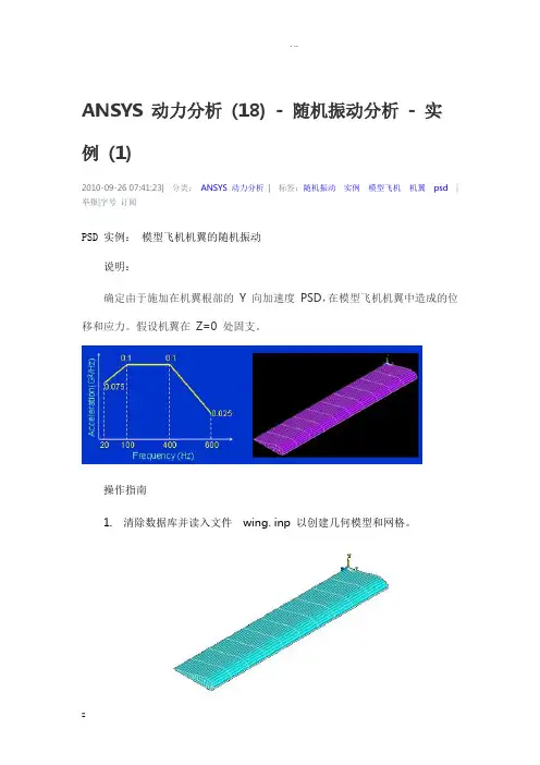
ANSYS 动力分析(18) - 随机振动分析- 实例(1)2010-09-26 07:41:23| 分类：ANSYS 动力分析| 标签：随机振动实例模型飞机机翼psd|举报|字号订阅PSD 实例：模型飞机机翼的随机振动说明：确定由于施加在机翼根部的Y 向加速度PSD，在模型飞机机翼中造成的位移和应力。

假设机翼在Z=0 处固支。

操作指南1. 清除数据库并读入文件wing. inp 以创建几何模型和网格。

2. 定义材料属性：弹性模量= 38000 psi 泊松比= 0.3密度= 1.033E-3/12 lbf-sec2/in4 = 8.6083E-53. 施加边界条件。

提示：选择在areas 上施加位移约束，拾取Z=0 处所有的Areas，约束所有自由度。

4. 定义新分析为Model，使用Block Lanczos 方法，抽取和扩展前15 个自然模态。

然后求解Current LS。

5. 查看模态形状，如图为前 4 阶振型。

6. 使用所显示的 PSD 谱，执行 PSD Spectrum 分析。

首先定义分析类型为 Spectrum分析类型为 PSD，使用全部模态，计算单元应力：注意激活“Calculate elem stresses”选项。

7. 在基础上施加指定的 PSD 谱 (注意：确保 PSD 的单位是 G2/Hz)。

施加 Y 向激励 (方法是：在基础节点上施加单位 Y 向位移)。

设置常阻尼比 0.02：设置有关参数–重力加速度值注意：响应谱类型选择 Accel (g**2/Hz)，否则后面的 PSD 谱应该输入实际加速度值：定义 PSD 谱表格：绘制 PSD 谱表格曲线以检查输入值：激活和设置模态组合参数：选择所有模态。

设置计算内容：计算各模态的参与因子:在输出窗口中可以看到参与因子的计算结果：求解：10. 在一般后处理中，查看相对位移和应力 (载荷步 3)。

首先查看 Results Summary：载荷步 3 为 set 17查看载荷步 3 的相对位移和应力：在 Read Results 中读取载荷步 3 的结果：使用 By set Number，输入 Data Set Number 为 17。

ansys abc随机振动仿真判定标准下载温馨提示：该文档是我店铺精心编制而成，希望大家下载以后，能够帮助大家解决实际的问题。

文档下载后可定制随意修改，请根据实际需要进行相应的调整和使用，谢谢!并且，本店铺为大家提供各种各样类型的实用资料，如教育随笔、日记赏析、句子摘抄、古诗大全、经典美文、话题作文、工作总结、词语解析、文案摘录、其他资料等等，如想了解不同资料格式和写法，敬请关注!Download tips: This document is carefully compiled by the editor. I hope that after you download them, they can help you solve practical problems. The document can be customized and modified after downloading, please adjust and use it according to actual needs, thank you!In addition, our shop provides you with various types of practical materials, suchas educational essays, diary appreciation, sentence excerpts, ancient poems, classic articles, topic composition, work summary, word parsing, copy excerpts, other materials and so on, want to know different data formats and writing methods, please pay attention!随机振动是指物体在受到外力的作用下呈现出的无规律的振动现象。

利用ANSYS随机振动分析功能实现随机疲劳分析
ANSYS随机振动分析功能可以获得结构随机振动响应过程的各种统计参数（如：
均值、均方根和平均频率等），根据各种随机疲劳寿命预测理论就可以成功地预测结
构的随机疲劳寿命。

本文介绍了ANSYS随机振动分析功能，以及利用该功能，按照Steinberg提出的基于高斯分布和Miner线性累计损伤定律的三区间法进行ANSYS随机疲劳计算的具体过程。

１．随机疲劳现象普遍存在
在工程应用中，汽车、飞行器、船舶以及其它各种机械或零部件，大多是在随机
载荷作用下工作，当它们承受的应力水平较高，工作达到一定时间后，经常会突然发
生随机疲劳破坏，往往造成灾难性的后果。

因此，预测结构或零部件的随机疲劳寿命
是非常有必要的。

2．ANSYS随机振动分析功能介绍
ANSYS随机振动分析功能十分强大，主要表现在以下方面：
1.具有位移、速度、加速度、力和压力等PSD类型；
2.能够考虑a阻尼、阻尼、恒定阻尼比和频率相关阻尼比；
3.能够定义基础和节点PSD激励；
4.能够考虑多个PSD激励之间的相关程度：共谱值、二次谱值、空间关系和波传
播关系等；
5.能够得到位移、应力、应变和力的三种结果数据： 1位移解，1速度解和
1加速度解；
3．利用ANSYS随机振动分析功能进行疲劳分析的一般原理
在工程界，疲劳计算广泛采用名义应力法，即以S-N曲线为依据进行寿命估算的
方法，可以直接得到总寿命。

下面围绕该方法举例说明ANSYS随机疲劳分析的一般原理。

ANSYS 动力分析(18) - 随机振动分析- 实例(1)2010-09-26 07:41:23| 分类：ANSYS 动力分析| 标签：随机振动实例模型飞机机翼psd|举报|字号订阅PSD 实例：模型飞机机翼的随机振动说明：确定由于施加在机翼根部的Y 向加速度PSD，在模型飞机机翼中造成的位移和应力。

假设机翼在Z=0 处固支。

操作指南1. 清除数据库并读入文件wing. inp 以创建几何模型和网格。

2. 定义材料属性：弹性模量= 38000 psi 泊松比= 0.3密度= 1.033E-3/12 lbf-sec2/in4 = 8.6083E-53. 施加边界条件。

提示：选择在areas 上施加位移约束，拾取Z=0 处所有的Areas，约束所有自由度。

4. 定义新分析为Model，使用Block Lanczos 方法，抽取和扩展前15 个自然模态。

然后求解Current LS。

5. 查看模态形状，如图为前 4 阶振型。

6. 使用所显示的 PSD 谱，执行 PSD Spectrum 分析。

首先定义分析类型为 Spectrum分析类型为 PSD，使用全部模态，计算单元应力：注意激活“Calculate elem stresses”选项。

7. 在基础上施加指定的 PSD 谱 (注意：确保 PSD 的单位是 G2/Hz)。

施加 Y 向激励 (方法是：在基础节点上施加单位 Y 向位移)。

设置常阻尼比 0.02：设置有关参数–重力加速度值注意：响应谱类型选择 Accel (g**2/Hz)，否则后面的 PSD 谱应该输入实际加速度值：定义 PSD 谱表格：绘制 PSD 谱表格曲线以检查输入值：激活和设置模态组合参数：选择所有模态。

设置计算内容：计算各模态的参与因子:在输出窗口中可以看到参与因子的计算结果：求解：10. 在一般后处理中，查看相对位移和应力 (载荷步 3)。

首先查看 Results Summary：载荷步 3 为 set 17查看载荷步 3 的相对位移和应力：在 Read Results 中读取载荷步 3 的结果：使用 By set Number，输入 Data Set Number 为 17。

第9章随机振动分析随机振动分析是一种基于概率统计学的谱分析技术，它求解的是在随机激励作用下的某些物理量，包括位移、应力等的概率分布情况等。

随机振动分析在机载电子设备、抖动光学设备、声学装载设备等方面有着广泛的应用。

★ 了解随机振动分析。

9.1随机振动分析概述随机振动分析（Random Vibration Analysis）是一种基于概率统计学的谱分析技术。

随机振动分析中功率谱密度（Power Spectral Density，PSD）记录了激励和响应的均方根值同频率的关系，因此PSD是一条功率谱密度值——频率值的关系曲线，如图9-1所示，亦即载荷时间历程。

图9-1 功率谱密度图第9章随机振动分析对PSD的说明如下。

PSD曲线下的面积就是方差，即响应标准偏差的平方值。

PSD的单位是Mean Square/Hz（如加速度PSD的单位为G2/Hz）。

PSD可以是位移、速度、加速度、力或者压力等。

在随机振动分析中，由于时间历程不是确定的，所以瞬态分析是不可用的。

随机振动分析的输入为：通过模态分析得到的结构固有频率和固有模态。

作用于节点的单点或多点的PSD激励曲线。

随机振动分析输出的是：作用于节点的PSD响应（位移和应力等），同时还能用于疲劳寿命预测。

9.2 随机振动分析流程在ANSYS Workbench左侧工具箱中Analysis Systems下的Random Vibration上按住鼠标左键拖动到项目管理区的A6栏，即可创建随机振动分析项目，如图9-2所示。

图9-2 创建随机振动分析项目当进入Mechanical后，选中分析树中的Analysis Settings即可进行分析参数的设置，如图9-3所示。

图9-3 随机振动分析参数设置。

振动疲劳—ansys随机振动疲劳分析随机振动疲劳分析流程图随机振动疲劳分析将第一步频率响应分析得到的结果文件作为输入，并在疲劳软件中输入振动过程中的PSD曲线，经计算得到零件的振动疲劳寿命。

故随机振动疲劳分析可分为如下步骤：1.频率响应分析结果输入2.功率谱密度PSD输入3.材料疲劳特性设置4.各工况与PSD关联设置5.振动疲劳求解器参数设置6.输出设置7.分析结果处理频率响应分析结果输入功率谱密度PSD输入振动疲劳求解器Ncode云图显示输出设置Ncode随机振动疲劳分析流程图1.频率响应分析结果输入频率响应分析应与PSD 的单位相对应，比如PSD 单位为g^2/Hz ，则进行频率响应分析时可输入1g 的加速度激励来分析。

（如采取单位制ton-mm-s-N ，此时1g 的加速度激励为9800mm/s^2，应在分析中输入9800大小的加速度激励）1.1单位问题1.2频率响应分析结果输出设置为了避免输出结果过大，可以在输出中设置需要进行疲劳分析的部件，以set 形式输出，同时可设置输出频次Frequency=n ，只输出频响分析应力结果即可。

*OUTPUT, FIELD, Frequency=5 *ELEMENT OUTPUT, ELSET = ele_setS, 以Abaqus 进行频响分析为例，输出设置如下：每5步输出一次只输出单元集合名为ele_set 的应力结果2.功率谱密度PSD输入PSD可以用以下2种方式输入：1.通过MultiColumnInput读入定义好的CSV文件输入2.通过VibrationGenerator生成PSD 曲线CSV文件格式如下：（可在帮助文档中找一个PSD的CSV文件作为模板）。

Random Vibration Analysis with ANSYSand VerificationByYe ZhouMay 2002Table of Contents1I NTRODUCTION TO R ANDOM V IBRATION (3)1.1Failure Modes in Random Vibration (3)1.2Random Vibration Input Curve and Units (3)1.3Normal Distribution Curve (4)1.4PSD for Fatigue Calculation (5)2F ORMULATION (6)2.1Steinberg formulation [1. 9.16]: (6)2.2Thomson formulation [2. 10.3]: (7)2.3Newland formulation [4. 7]: (7)3ANSYS P ROCEDURES (8)4R EFERENCES (10)5A PPENDIX –ANSYS PSD I NPUT/O UTPUT F ILE (11)5.1Input File (11)5.2Output File (13)List of FiguresFigure 1 Typical white noise curve with a constant input power spectral density (PSD) (4)Figure 2 Sample 1-DOF model (6)Figure 3 ANSYS calculated output PSD (8)List of TablesTable 1 Type of spectral densities (4)Table 2 Safety index/sigma values used in building codes (6)Table 3 ANSYS results verification (9)Table 4 ANSYS PSD result load steps (9)1 Introduction to Random VibrationRandom vibration is being specified for acceptance and qualification tests by many institutions, because it has been shown that random vibration more closely represents the true environments in which the structures and equipment must operate. 1.1Failure Modes in Random VibrationThere are four basic failure modes that must be considered under random vibration. These failures are:1. High acceleration levels.2. High stress levels.3. Large displacement amplitudes.4. Electrical signals out of tolerance (electrical component only). 1.2Random Vibration Input Curve and UnitsThere are many different types of curves that can be used to show the random vibration input requirements. The most common curve, which is also the simplest, is the white-noise curve shown in Figure 1.Random vibration input and response curves are typically plotted on log-log paper, with the power spectral density expressed squared acceleration units per Hertz, such as g 2/Hz. The power spectral density P is often referred as the mean squared acceleration density, and it is defined as:fG P f ∆=→∆20lim where G is the root mean square (RMS) of the acceleration expressed in gravity units.Root mean square acceleration levels are related to the area under the random vibration curve. The input RMS acceleration levels can be obtained by integrating under the input random vibration curve, and the output (or response) RMS acceleration levels can be obtained by integrating under the output or response random vibration curve. The square root of the area then determined the RMS acceleration level, with units:RMS G G Hz HzG Area 22==⨯=For example, the input RMS acceleration level resulting from the white-noise random vibration input specification shown in Figure 1 is calculated as follows:0.3)10100(1.0=-=∆⨯=f P G RMS (RMS input acceleration level)Random vibration environments in the industry normally deal in terms of the power spectral density P (or mean squared acceleration density), which is measured in gravity units so that it is dimensionless: gravityon accelerati g a G ==(dimensionless)An acceleration level of 10G means that the acceleration has a magnitude that is 10 times greater than the acceleration of gravity.Random vibration sometimes is also expressed in terms of velocity or displacement spectral density as defined in Table 1.Figure 1 Typical white noise curve with a constant input power spectral density (PSD)Table 1 Type of spectral densities1.3 Normal Distribution CurveThe Gaussian distribution curve represents the probability for the value of the instantaneous acceleration levels at any time. The abscissa is the ratio of the instantaneous acceleration to the RMS acceleration, and the ordinate is the probability density, sometimes called probability of occurrences. The total area under the curve is unity.From the nature of Gaussian distribution, the instantaneous acceleration will exceed the 1σ, which is the RMS value, 31.7% of the time. It will exceed the 2σ value, which is two times the RMS value, 4.6% of the time. It will exceed the 3σ value which is three time the RMS value, 0.27% of the time.The maximum acceleration levels considered for random vibrations are the 3σ levels [1. 9.13], because the instantaneous accelerations are between the +3σ and the -3σ levels 99.73% of the time, which is very close to 100% of the time. Higher acceleration levels of 4σ and 5σ can occur in the real world, but they are usually ignored because most test equipment for random vibration have 3σ clippers built into the electronic control systems. These clippers limit the input acceleration levels to values that are 3 times greater than the RMS input levels.When a 10G RMS random vibration environment is being evaluated, input or response, then 2σaccelerations of 20G can be expected some of the time, and 3σ accelerations of 30G can be expected some of the time.Random vibration qualification tests performed in a laboratory will typically be run using much higher acceleration levels than the values found in the actual environments [1. 9.13]. The laboratory may use input test levels of 8.0G RMS for a period of 2 hours, to try to accumulate the same amount of damage that is expected in a 1.5G RMS environment over a 15-year period. Random vibration qualification tests are often considered to be accelerated life tests.1.4 PSD for Fatigue CalculationUsing results from random vibrations to evaluate fatigue life is used in many design guidelines such as Ref.3. Engineers use σ values varying from 2 to 3, or multi-band technique, for fatigue calculation. Choosing high σ values for fatigue calculation is more a matter of conservatism than a matter of correctness.1.4.1Three band techniqueThree-band technique is a simplified approach to the evaluation of random vibration fatigue [1. 9.14]. The basis for the three-band techniq ue is the Gaussian distribution. The Miner’s Rule can be applied to the following frequency categories:∙1σ values occur 68.3% of the time.∙2σ values occur 27.1% of the time (95.4%-68.3%=27.1%).∙3σ values occur 4.33% of the time (99.73%-95.4%=4.33%).1.4.2Fatigue load compared to Building CodesMany limit states based building codes divides the loading conditions into two states: serviceability and ultimate states, where serviceability state is used for calculation of fatigue, deflection, etc. North American building codes use the safety index as defined in Table 2. A safety index of x is corresponding to an xσresponse level.Table 2 Safety index/sigma values used in building codes2 FormulationThe formulation of a random vibration analysis can be illustrated by a simple 1-DOF example shown in Figure 2. The example calculation is based on the PSD shown in Figure 1.k 1 = 42832 lb/in m 1 = 0.5 lb-sec 2/inξ=0.02Figure 2 Sample 1-DOF modelMany classic textbooks [1. 9.16][2. 10.3] prescribe the input spectral density as in acceleration (g 2/Hz), and others use input spectral density as in force (force 2/Hz). The following sections describe three variations of formulations. 2.1Steinberg formulation [1. 9.16]:⎰=212f f out out df P GP out =Q 2PWhere P is input PSD in units of G 2/Hz, G is the output acceleration level in units of length/second 2. And Q is the transmissibility of a 1DOF system:22222)2()1()2(1⎥⎥⎦⎤⎢⎢⎣⎡+-+=ΩΩΩc c R R R R R Q where R Ω=Ω/Ωn , and R c =damping ratio ξfor a lightly damped system, R c 2=0211Ω-=R QThus,[][]⎰+-=212222)/(2)/(1f f nn out df f f f f PG ξand ξπ402Pf df P G n out out ==⎰∞(Eq. 1)for a lightly damped system, ξ=1/(2Q ), thusn n out Q Pf G 2π=(RMS), (Eq. 2)where subscript n refers to quantities at the resonance frequency.Using the Equation 2, we can calculate the response acceleration RMS of the sample 1-DOF problem as follows:02.25)04.0()04.0(1)2()2(121222122=⎪⎪⎭⎫⎝⎛+=⎪⎪⎭⎫⎝⎛+=ξξn Qg inchinch Q Pf G n n out 53.13sec7.519502.25sec 1582.46sec 6.1474522232==⋅⋅⋅==ππThen the base reaction is Reaction= Wt ⋅ Acceleration = 0.5 lbf-sec 2/inch ⋅ 386 inch/sec 2 ⋅ 5195.7 inch/sec 2 = 2598 lbf .2.2Thomson formulation [2. 10.3]:The Steinberg formulation can be also written as:⎰⎰==2121)()()()()()(**2f f out dff H f H f S d H H S G ωωωωωωwhere S (ω) is written as P (ω) in Steinberg formulation.[][])/(2)/(11)(2nn f f i f f f H ξ+-=2.3Newland formulation [4. 7]:In Reference 4. D. E. Newland expresses the spectral density S in terms of forces, as defined in the baseequation of motion:)(t x ky y c ym =++ (Eq. 3)where x(t)is the excitation force.The formulation for response RMS is as follows:02)()(S H S y ωω=where S 0 = S x (ω) is the spectral density of the forcing function x (t ), and H (ω) is the complex frequency response function. H (ω) can be derived by putting x (t )=e i ωt and y (t )= H (ω) e i ωt into equation 3:kic m H ++-=ωωω21)(Hence the output spectral density is22220)()(ωωωc m k S S y +-=and the mean square of the output spectrum is ⎰++-=2102221][ωωωωωd S kic m y E3 ANSYS ProceduresAn ANSYS input file for calculating the 1-DOF example shown in Figure 1 and 2 is attached in the Appendix. This input file was tested using ANSYS 6.0 Multiphysics. The output response spectrum is shown in Figure 3. The input file was modified from ANSYS Verification Example VM68.Figure 3 ANSYS calculated output PSDThe ANSYS results are compared with those of the theoretical calculation in the previous sections, shown in Table 3.Table 3 ANSYS results verificationAfter a successful PSD analysis, ANSYS exports results into several load steps as shown in Table 4. Results from load step 3-1 and 5-1 are of interest to the example discussed here. Load step 3-1 gives the 1σ RMS displacement, base reactions and member stresses. Nodal displacement output in load step 5-1 actually gives the 1σ RMS acceleration at the nodes.Table 4 ANSYS PSD result load steps4 References1. Dave S. Steinberg, Vibration Analysis for Electronic Equipment, 3rd Ed. John Wiley & Sons 2000UBCLIB TK7870.S8218 2000Clear and no-nonsense explanation on random vibration analysis. Practical design advice and notes on fatigue design.2. William T. Thomson, Vibration Theory and Applications, Prentice-Hall 1965UBCLIB TA355.T47 1965Classic textbook with numerical examples.3. NASA Preferred Reliability Practices, Gudeline No. GD-AP-2303, Spectral Fatigue Reliability,Johnson Space Center, USA4. D. E. Newland, An Introduction to Random Vibrations and Spectral Analysis, 2nd Ed. LongmanScience & Technical 1984UBCLIB QA935.N46 1984Complete and accurate documentation on all formulas.5 Appendix – ANSYS PSD Input/Output File5.1 Input Filec r e a t eF I N I S H!F E A e l e m e n t s o f t h e C V/C L E A R,S T A R T/P R E P7/T I T L E,C V B e a m E l e m e n t F E AA N T Y P E,S T A T I CE T,1,C O M B I N40!D I S P L A C E M E N T A L O N G X A X I S,M A S S A T N O D E IR,1,42832.,,0.50M P,E X,1,1!N O T U S E D,D U M M Y P R O P E R T YN,1!D E F I N E M O D E LN,2,1E,2,1D,1,U X,0.0!C O N S T R A I N T T H E B A S EO U T P R,A L L,A L LF I N I S H/e o fs o l v P S D/S O L UA N T Y P E,M O D A L!P E R F O R M A M O D A L A N A L Y S I SM O D O P T,S U B S P,1!S U B S P A C E I E R T A T I O N M E T H O D!E X T R A C T2M O D E S F R O M E N T I R E F R E Q U E N C Y R A N G E M X P A N D,1,,,Y E S!E X P A N D2M O D E S,D O E L E M E N T S T R E S S C A L C U L A T I O N SS O L V E*G E T,F R E Q1,M O D E,1,F R E QF I N I S H/S O L UA N T Y P E,S P E C T R!P E R F O R M S P E C T R U M A N A L Y S I SS P O P T,P S D,2,O N!U S E F I R S T2M O D E S F R O M M O D A L A N A L Y S I SP S D U N I T,1,A C C G!U S E G**2/H Z F O R P S D A N D D I M E N S I O N I N I N C H E SD,1,U X,1.0!A P P L Y S P E C T R U M A T T H E S U P P O R T P O I N TP S D F R Q,1,1,10.0,100.0!F R E Q U E N C Y R A N G E O F10T O100H E R T ZP S D V A L,1,.1,.1!W H I T E N O I S E P S D,V A L U E S I N G**2/H ZP F A C T,1,B A S E!B A S E E X C I T A T I O ND M P R A T,0.02!2%D A M P I N GP S D C O M!C O M B I N E M O D E S F O R P S D,U S E D E F A U L T S I G N I F I C A N C E L E V E LP S D R E S,A C E L,R E L!C A L C U L A T E R E L A T I V E A C C E L E R A T I O N S O L U T I O N SS O L V EF I N I S H/e o fp o s t v mf i n i s h/P O S T1L C D E F,6,5,1!D E F I N E L O A D S T E P A N D S U B S T E P F O R L O A D F A C T O R O P E R A T I O NL C F A C T,A L L,(1/386.4)!C O N V E R T A C C E L.R E S U L T T O GL C A S E,6P R N S O L,U,C O M P!P R I N T N O D A L S O L U T I O N R E S U L T S*G E T,M1S T D,N O D E,2,U,X*D I M,L A B E L,C H A R,4,2*D I M,V A L U E,,2,3L A B E L(1,1)='f1,','A C C1S I G'L A B E L(1,2)='H z','g'*V F I L L,V A L U E(1,1),D A T A,46.58,13.53*V F I L L,V A L U E(1,2),D A T A,F R E Q1,M1S T D*V F I L L,V A L U E(1,3),D A T A,A B S(F R E Q1/46.58),A B S(M1S T D/13.53)/C O M/O U T,v m68,v r t/C O M,-------------------V M68R E S U L T S C O M P A R I S O N--------------/C O M,/C O M,|T A R G E T|A N S Y S|R A T I O/C O M,*V W R I T E,L A B E L(1,1),L A B E L(1,2),V A L U E(1,1),V A L U E(1,2),V A L U E(1,3) (1X,A8,A8,'',F10.3,'',F10.3,'',1F5.3)/C O M,----------------------------------------------------------s e t,3,1p r d i s pp r r s o ls e t,5,1p r d i s p/O U TF I N I S H*L I S T,v m68,v r t/e o fp s d o u tF I N I S H/p o s t26n u m N S e t=2*d e l,n o d e P l*d i m,n o d e P l,a r r a y,n u m N S e tn o d e P l(1)=2n o d e P l(2)=1*d o,i P s d o,1,n u m N S e t,1/T I T L E,R E S P O N S E v s I N P U T S P E C T R U MR E S E TS T O R E,P S D,8N S O L,2,1,U,x,b a s eN S O L,3,n o d e P l(i P s d o),U,x,n o d e2R P S D,4,2,,3,1,R P S D B A SR P S D,5,3,,3,1,R P S D R F!B E L O W I S R E L A T I V E R E S P O N S ER P S D,6,3,,3,2,R P S D R F RP L T I M E,0,2500/G R O P T,L O G X,O N/G R O P T,L O G Y,O N/A X L A B,X,F r e q u e n c y(H z)/A X L A B,Y,P S D G^2/H z!p l v a r,4,5!!N O T E:D I V I D E O U T P U T L I K E298.61I N^2/S E C^4/H Z B Y386.4^2T O G E T B A C K T O g^2/H Z-S E E!B E L O WP R O D,7,4,,,R P S D B A S E,,,1/386.4**2,1,1,P R O D,8,5,,,R P S D R F R,,,1/386.4**2,1,1,!P L O T R E S P O N S E P S D V E R S U S I N P U T P S Dp l v a r,7,8/S H O W,P N GP N G R,C O M P,1,-1P N G R,O R I E N T,H O R I ZP N G R,C O L O R,2P N G R,T M O D,1/G F I L E,1200,!*/C M A P,_T E M P C M A P_,C M P,,S A V E/R G B,I N D E X,100,100,100,0/R G B,I N D E X,0,0,0,15p l v a r,7,8/C M A P,_T E M P C M A P_,C M P/D E L E T E,_T E M P C M A P_,C M P/S H O W,C L O S E/D E V I C E,V E C T O R,0/t i t l e,c o n V a n P S D*e n d d o/e o f5.2 Output File-------------------V M68R E S U L T S C O M P A R I S O N--------------|T A R G E T|A N S Y S|R A T I Of1,H z46.58046.5821.000A C C1S I G g13.53013.7011.013----------------------------------------------------------U S E L O A D S T E P3S U B S T E P1F O R L O A D C A S E0S E T C O M M A N D G O T L O A D S T E P=3S U B S T E P=1C U M U L A T I V E I T E R A T I O N=3T I M E/F R E Q U E N C Y=0.0000T I T L E=C V B e a m E l e m e n t F E AP R I N T D O F N O D A L S O L U T I O N P E R N O D E*****P O S T1N O D A L D E G R E E O F F R E E D O M L I S T I N G*****L O A D S T E P=3S U B S T E P=1F R E Q=0.0000L O A D C A S E=0T H E F O L L O W I N G D E G R E E O F F R E E D O M R E S U L T S A R E I N N O D A L C O O R D I N A T E SN O D E U X10.000020.60799E-01M A X I M U M A B S O L U T E V A L U E SN O D E2V A L U E0.60799E-01P R I N T R E A C T I O N S O L U T I O N S P E R N O D E*****P O S T1T O T A L R E A C T I O N S O L U T I O N L I S T I N G*****L O A D S T E P=3S U B S T E P=1F R E Q=0.0000L O A D C A S E=0T H E F O L L O W I N G X,Y,Z S O L U T I O N S A R E I N N O D A L C O O R D I N A T E SN O D E F X12604.2T O T A L V A L U E SV A L U E2604.2U S E L O A D S T E P5S U B S T E P1F O R L O A D C A S E0S E T C O M M A N D G O T L O A D S T E P=5S U B S T E P=1C U M U L A T I V E I T E R A T I O N=4 T I M E/F R E Q U E N C Y=0.0000T I T L E=C V B e a m E l e m e n t F E AP R I N T D O F N O D A L S O L U T I O N P E R N O D E*****P O S T1N O D A L D E G R E E O F F R E E D O M L I S T I N G*****L O A D S T E P=5S U B S T E P=1F R E Q=0.0000L O A D C A S E=0T H E F O L L O W I N G D E G R E E O F F R E E D O M R E S U L T S A R E I N N O D A L C O O R D I N A T E SN O D E U X10.000025294.2M A X I M U M A B S O L U T E V A L U E SN O D E2V A L U E5294.2。