投资学10

CHAPTER 7: OPTIMAL RISKY PORTFOLIOSPROBLEM SETS1. (a) and (e). Short-term rates and labor issues are factors thatare common to all firms and therefore must be considered as market risk factors. The remaining three factors are unique to this corporation and are not a part of market risk.2. (a) and (c). After real estate is added to the portfolio, there arefour asset classes in the portfolio: stocks, bonds, cash, and real estate. Portfolio variance now includes a variance term for real estate returns and a covariance term for real estate returns with returns for each of the other three asset classes. Therefore,portfolio risk is affected by the variance (or standard deviation) of real estate returns and the correlation between real estatereturns and returns for each of the other asset classes. (Note that the correlation between real estate returns and returns for cash is most likely zero.)3. (a) Answer (a) is valid because it provides the definition of theminimum variance portfolio.4. The parameters of the opportunity set are:E (r S ) = 20%, E (r B ) = 12%, σS = 30%, σB = 15%, ρ =From the standard deviations and the correlation coefficient we generate the covariance matrix [note that (,)S B S B Cov r r ρσσ=⨯⨯]: Bonds Stocks Bonds 225 45 Stocks 45 900The minimum-variance portfolio is computed as follows:w Min (S ) =1739.0)452(22590045225)(Cov 2)(Cov 222=⨯-+-=-+-B S B S B S B ,r r ,r r σσσ w Min (B ) = 1 =The minimum variance portfolio mean and standard deviation are:E (r Min ) = × .20) + × .12) = .1339 = %σMin = 2/12222)],(Cov 2[B S B S B B S Sr r w w w w ++σσ = [ 900) + 225) + (2 45)]1/2= %5.Proportion in Stock Fund Proportionin Bond Fund ExpectedReturnStandard Deviation% % % %minimumtangencyGraph shown below.0.005.0010.0015.0020.0025.000.00 5.00 10.00 15.00 20.00 25.00 30.00Tangency PortfolioMinimum Variance PortfolioEfficient frontier of risky assetsCMLINVESTMENT OPPORTUNITY SETr f = 8.006. The above graph indicates that the optimal portfolio is thetangency portfolio with expected return approximately % andstandard deviation approximately %.7. The proportion of the optimal risky portfolio invested in the stockfund is given by:222[()][()](,)[()][()][()()](,)S f B B f S B S S f B B f SS f B f S B E r r E r r Cov r r w E r r E r r E r r E r r Cov r r σσσ-⨯--⨯=-⨯+-⨯--+-⨯[(.20.08)225][(.12.08)45]0.4516[(.20.08)225][(.12.08)900][(.20.08.12.08)45]-⨯--⨯==-⨯+-⨯--+-⨯10.45160.5484B w =-=The mean and standard deviation of the optimal risky portfolio are:E (r P ) = × .20) + × .12) = .1561 = % σp = [ 900) +225) + (2× 45)]1/2= %8. The reward-to-volatility ratio of the optimal CAL is:().1561.080.4601.1654p fpE r r σ--==9. a. If you require that your portfolio yield an expected return of14%, then you can find the corresponding standard deviation from the optimal CAL. The equation for this CAL is:()().080.4601p fC f C C PE r r E r r σσσ-=+=+If E (r C ) is equal to 14%, then the standard deviation of the portfolio is %.b. To find the proportion invested in the T-bill fund, rememberthat the mean of the complete portfolio ., 14%) is an average of the T-bill rate and the optimal combination of stocks and bonds (P ). Let y be the proportion invested in the portfolio P . The mean of any portfolio along the optimal CAL is:()(1)()[()].08(.1561.08)C f P f P f E r y r y E r r y E r r y =-⨯+⨯=+⨯-=+⨯-Setting E (r C ) = 14% we find: y = and (1 − y ) = (the proportion invested in the T-bill fund).To find the proportions invested in each of the funds, multiply times the respective proportions of stocks and bonds in the optimal risky portfolio:Proportion of stocks in complete portfolio = =Proportion of bonds in complete portfolio = =10. Using only the stock and bond funds to achieve a portfolio expectedreturn of 14%, we must find the appropriate proportion in the stock fund (w S) and the appropriate proportion in the bond fund (w B = 1 −w S) as follows:= × w S + × (1 −w S) = + × w S w S =So the proportions are 25% invested in the stock fund and 75% inthe bond fund. The standard deviation of this portfolio will be:σP = [ 900) + 225) + (2 45)]1/2 = %This is considerably greater than the standard deviation of %achieved using T-bills and the optimal portfolio.11. a.Even though it seems that gold is dominated by stocks, gold mightstill be an attractive asset to hold as a part of a portfolio. Ifthe correlation between gold and stocks is sufficiently low, goldwill be held as a component in a portfolio, specifically, theoptimal tangency portfolio.b.If the correlation between gold and stocks equals +1, then no onewould hold gold. The optimal CAL would be composed of bills andstocks only. Since the set of risk/return combinations of stocksand gold would plot as a straight line with a negative slope (seethe following graph), these combinations would be dominated bythe stock portfolio. Of course, this situation could not persist.If no one desired gold, its price would fall and its expectedrate of return would increase until it became sufficientlyattractive to include in a portfolio.12. Since Stock A and Stock B are perfectly negatively correlated, arisk-free portfolio can be created and the rate of return for thisportfolio, in equilibrium, will be the risk-free rate. To find theproportions of this portfolio [with the proportion w A invested inStock A and w B = (1 –w A) invested in Stock B], set the standarddeviation equal to zero. With perfect negative correlation, theportfolio standard deviation is:σP = Absolute value [w AσA w BσB]0 = 5 × w A− [10 (1 –w A)] w A =The expected rate of return for this risk-free portfolio is:E(r) = × 10) + × 15) = %Therefore, the risk-free rate is: %13. False. If the borrowing and lending rates are not identical, then,depending on the tastes of the individuals (that is, the shape oftheir indifference curves), borrowers and lenders could havedifferent optimal risky portfolios.14. False. The portfolio standard deviation equals the weighted averageof the component-asset standard deviations only in the special case that all assets are perfectly positively correlated. Otherwise, as the formula for portfolio standard deviation shows, the portfoliostandard deviation is less than the weighted average of thecomponent-asset standard deviations. The portfolio variance is aweighted sum of the elements in the covariance matrix, with theproducts of the portfolio proportions as weights.15. The probability distribution is:Probability Rate ofReturn100%−50Mean = [ × 100%] + [ × (-50%)] = 55%Variance = [ × (100 − 55)2] + [ × (-50 − 55)2] = 4725Standard deviation = 47251/2 = %16. σP = 30 = y× σ = 40 × y y =E(r P) = 12 + (30 − 12) = %17. The correct choice is (c). Intuitively, we note that since allstocks have the same expected rate of return and standard deviation, we choose the stock that will result in lowest risk. This is thestock that has the lowest correlation with Stock A.More formally, we note that when all stocks have the same expected rate of return, the optimal portfolio for any risk-averse investor is the global minimum variance portfolio (G). When the portfolio is restricted to Stock A and one additional stock, the objective is to find G for any pair that includes Stock A, and then select thecombination with the lowest variance. With two stocks, I and J, theformula for the weights in G is:)(1)(),(Cov 2),(Cov )(222I w J w r r r r I w Min Min J I J I J I J Min -=-+-=σσσSince all standard deviations are equal to 20%:(,)400and ()()0.5I J I J Min Min Cov r r w I w J ρσσρ====This intuitive result is an implication of a property of any efficient frontier, namely, that the covariances of the global minimum variance portfolio with all other assets on the frontier are identical and equal to its own variance. (Otherwise, additional diversification would further reduce the variance.) In this case, the standard deviation of G(I, J) reduces to:1/2()[200(1)]Min IJ G σρ=⨯+This leads to the intuitive result that the desired addition would be the stock with the lowest correlation with Stock A, which is Stock D. The optimal portfolio is equally invested in Stock A and Stock D, and the standard deviation is %.18. No, the answer to Problem 17 would not change, at least as long asinvestors are not risk lovers. Risk neutral investors would not care which portfolio they held since all portfolios have an expected return of 8%.19. Yes, the answers to Problems 17 and 18 would change. The efficientfrontier of risky assets is horizontal at 8%, so the optimal CAL runs from the risk-free rate through G. This implies risk-averse investors will just hold Treasury bills.20. Rearrange the table (converting rows to columns) and compute serialcorrelation results in the following table:Nominal RatesFor example: to compute serial correlation in decade nominalreturns for large-company stocks, we set up the following twocolumns in an Excel spreadsheet. Then, use the Excel function“CORREL” to calculate the correlation for the data.Decade Previous1930s%%1940s%%1950s%%1960s%%1970s%%1980s%%1990s%%Note that each correlation is based on only seven observations, so we cannot arrive at any statistically significant conclusions.Looking at the results, however, it appears that, with theexception of large-company stocks, there is persistent serialcorrelation. (This conclusion changes when we turn to real rates in the next problem.)21. The table for real rates (using the approximation of subtracting adecade’s average inflation from the decade’s average nominalreturn) is:Real RatesSmall Company StocksLarge Company StocksLong-TermGovernmentBondsIntermed-TermGovernmentBondsTreasuryBills 1920s1930s1940s1950s1960s1970s1980s1990sSerialCorrelationWhile the serial correlation in decade nominal returns seems to be positive, it appears that real rates are serially uncorrelated. The decade time series (although again too short for any definitiveconclusions) suggest that real rates of return are independent from decade to decade.22. The 3-year risk premium for the S&P portfolio is, the 3-year risk premium for thehedge fund portfolio is S&P 3-year standard deviation is 0. The hedge fund 3-year standard deviation is 0. S&P Sharpe ratio is = , and the hedge fund Sharpe ratio is = .23. With a ρ = 0, the optimal asset allocation is,.With these weights,EThe resulting Sharpe ratio is = . Greta has a risk aversion of A=3, Therefore, she will investyof her wealth in this risky portfolio. The resulting investment composition will be S&P: = % and Hedge: = %. The remaining 26% will be invested in the risk-free asset.24. With ρ = , the annual covariance is .25. S&P 3-year standard deviation is . The hedge fund 3-year standard deviation is . Therefore, the 3-year covariance is 0.26. With a ρ=.3, the optimal asset allocation is, .With these weights,E. The resulting Sharpe ratio is = . Notice that the higher covariance results in a poorer Sharpe ratio.Greta will investyof her wealth in this risky portfolio. The resulting investment composition will be S&P: =% and hedge: = %. The remaining % will be invested in the risk-free asset.CFA PROBLEMS1. a. Restricting the portfolio to 20 stocks, rather than 40 to 50stocks, will increase the risk of the portfolio, but it ispossible that the increase in risk will be minimal. Suppose that, for instance, the 50 stocks in a universe have the same standard deviation () and the correlations between each pair areidentical, with correlation coefficient ρ. Then, the covariance between each pair of stocks would be ρσ2, and the variance of an equally weighted portfolio would be:222ρσ1σ1σnn n P -+=The effect of the reduction in n on the second term on theright-hand side would be relatively small (since 49/50 is close to 19/20 and ρσ2 is smaller than σ2), but thedenominator of the first term would be 20 instead of 50. For example, if σ = 45% and ρ = , then the standard deviation with 50 stocks would be %, and would rise to % when only 20 stocks are held. Such an increase might be acceptable if the expected return is increased sufficiently.b. Hennessy could contain the increase in risk by making sure thathe maintains reasonable diversification among the 20 stocks that remain in his portfolio. This entails maintaining a low correlation among the remaining stocks. For example, in part (a), with ρ = , the increase in portfolio risk was minimal. As a practical matter, this means that Hennessy would have to spread his portfolio among many industries; concentrating on just a few industries would result in higher correlations among the included stocks.2. Risk reduction benefits from diversification are not a linearfunction of the number of issues in the portfolio. Rather, the incremental benefits from additional diversification are mostimportant when you are least diversified. Restricting Hennessy to 10 instead of 20 issues would increase the risk of his portfolio by a greater amount than would a reduction in the size of theportfolio from 30 to 20 stocks. In our example, restricting the number of stocks to 10 will increase the standard deviation to %. The % increase in standard deviation resulting from giving up 10 of20 stocks is greater than the % increase that results from givingup 30 of 50 stocks.3. The point is well taken because the committee should be concernedwith the volatility of the entire portfolio. Since Hennessy’sportfolio is only one of six well-diversified portfolios and issmaller than the average, the concentration in fewer issues mighthave a minimal effect on the diversification of the total fund.Hence, unleashing Hennessy to do stock picking may be advantageous.4. d. Portfolio Y cannot be efficient because it is dominated byanother portfolio. For example, Portfolio X has both higherexpected return and lower standard deviation.5. c.6. d.7. b.8. a.9. c.10. Since we do not have any information about expected returns, wefocus exclusively on reducing variability. Stocks A and C have equal standard deviations, but the correlation of Stock B with Stock C is less than that of Stock A with Stock B . Therefore, a portfoliocomposed of Stocks B and C will have lower total risk than aportfolio composed of Stocks A and B.11. Fund D represents the single best addition to complementStephenson's current portfolio, given his selection criteria. Fund D’s expected return percent) has the potential to increase theportfolio’s return somewhat. Fund D’s relatively low correlation with his current portfolio (+ indicates that Fund D will providegreater diversification benefits than any of the other alternativesexcept Fund B. The result of adding Fund D should be a portfolio with approximately the same expected return and somewhat lower volatility compared to the original portfolio.The other three funds have shortcomings in terms of expected return enhancement or volatility reduction through diversification. Fund A offers the potential for increasing the portfolio’s return but is too highly correlated to provide substantial volatility reduction benefits through diversification. Fund B provides substantial volatility reduction through diversification benefits but is expected to generate a return well below the current portfolio’s return. Fund C has the greatest potential to increase the portfolio’s return but is too highly correlated with the current portfolio to provide substantial volatility reduction benefits through diversification.12. a. Subscript OP refers to the original portfolio, ABC to thenew stock, and NP to the new portfolio.i. E(r NP) = w OP E(r OP) + w ABC E(r ABC) = + = %ii. Cov = ρOP ABC = =iii. NP = [w OP2OP2 + w ABC2ABC2 + 2 w OP w ABC(Cov OP , ABC)]1/2= [ 2 + + (2 ]1/2= % %b. Subscript OP refers to the original portfolio, GS to governmentsecurities, and NP to the new portfolio.i. E(r NP) = w OP E(r OP) + w GS E(r GS) = + = %ii. Cov = ρOP GS = 0 0 = 0iii. NP = [w OP2OP2 + w GS2GS2 + 2 w OP w GS (Cov OP , GS)]1/2= [ + 0) + (2 0)]1/2= % %c. Adding the risk-free government securities would result in alower beta for the new portfolio. The new portfolio beta will bea weighted average of the individual security betas in theportfolio; the presence of the risk-free securities would lowerthat weighted average.d. The comment is not correct. Although the respective standarddeviations and expected returns for the two securities underconsideration are equal, the covariances between each security andthe original portfolio are unknown, making it impossible to drawthe conclusion stated. For instance, if the covariances aredifferent, selecting one security over the other may result in alower standard deviation for the portfolio as a whole. In such acase, that security would be the preferred investment, assumingall other factors are equal.e. i. Grace clearly expressed the sentiment that the risk of losswas more important to her than the opportunity for return. Usingvariance (or standard deviation) as a measure of risk in her casehas a serious limitation because standard deviation does notdistinguish between positive and negative price movements.ii. Two alternative risk measures that could be used instead ofvariance are:Range of returns, which considers the highest and lowestexpected returns in the future period, with a larger rangebeing a sign of greater variability and therefore of greaterrisk.Semivariance can be used to measure expected deviations ofreturns below the mean, or some other benchmark, such as zero.Either of these measures would potentially be superior tovariance for Grace. Range of returns would help to highlightthe full spectrum of risk she is assuming, especially thedownside portion of the range about which she is so concerned.Semivariance would also be effective, because it implicitlyassumes that the investor wants to minimize the likelihood ofreturns falling below some target rate; in Grace’s case, thetarget rate would be set at zero (to protect against negativereturns).13. a. Systematic risk refers to fluctuations in asset prices causedby macroeconomic factors that are common to all risky assets;hence systematic risk is often referred to as market risk.Examples of systematic risk factors include the business cycle,inflation, monetary policy, fiscal policy, and technologicalchanges.Firm-specific risk refers to fluctuations in asset pricescaused by factors that are independent of the market, such asindustry characteristics or firm characteristics. Examples offirm-specific risk factors include litigation, patents,management, operating cash flow changes, and financial leverage.b. Trudy should explain to the client that picking only the topfive best ideas would most likely result in the client holdinga much more risky portfolio. The total risk of a portfolio, orportfolio variance, is the combination of systematic risk andfirm-specific risk.The systematic component depends on the sensitivity of theindividual assets to market movements as measured by beta.Assuming the portfolio is well diversified, the number ofassets will not affect the systematic risk component ofportfolio variance. The portfolio beta depends on theindividual security betas and the portfolio weights of those securities.On the other hand, the components of firm-specific risk (sometimes called nonsystematic risk) are not perfectly positively correlated with each other and, as more assets are added to the portfolio, those additional assets tend to reduce portfolio risk. Hence, increasing the number of securities in a portfolio reduces firm-specific risk. For example, a patent expiration for one company would not affect the othersecurities in the portfolio. An increase in oil prices islikely to cause a drop in the price of an airline stock butwill likely result in an increase in the price of an energy stock. As the number of randomly selected securities increases, the total risk (variance) of the portfolio approaches its systematic variance.。

CHAPTER 7: OPTIMAL RISKY PORTFOLIOSPROBLEM SETS1.(a) and (e). Short-term rates and labor issues are factors that are common to all firms and therefore must be considered as market risk factors. The remaining three factors are unique to this corporation and are not a part of market risk.2.(a) and (c). After real estate is added to the portfolio, there are four asset classes in the portfolio: stocks, bonds, cash, and real estate. Portfolio variance now includes a variance term for real estate returns and a covariance term for real estate returns with returns for each of the other three asset classes. Therefore, portfolio risk is affected by the variance (or standard deviation) of real estate returns and thecorrelation between real estate returns and returns for each of the other asset classes. (Note that the correlation between real estate returns and returns for cash is most likely zero.)3.(a) Answer (a) is valid because it provides the definition of the minimum variance portfolio.4.The parameters of the opportunity set are:E (r S ) = 20%, E (r B ) = 12%, σS = 30%, σB = 15%, ρ = 0.10From the standard deviations and the correlation coefficient we generate the covariance matrix [note that ]:(,)S B S B Cov r r ρσσ=⨯⨯Bonds StocksBonds 22545Stocks45900The minimum-variance portfolio is computed as follows:w Min (S ) =1739.0)452(22590045225)(Cov 2)(Cov 222=⨯-+-=-+-B S B S B S B ,r r ,r r σσσw Min (B ) = 1 - 0.1739 = 0.8261The minimum variance portfolio mean and standard deviation are:E (r Min ) = (0.1739 × .20) + (0.8261 × .12) = .1339 = 13.39%σMin = 2/12222)],(Cov 2[B S B S B B S S r r w w w w ++σσ= [(0.17392 ⨯ 900) + (0.82612 ⨯ 225) + (2 ⨯ 0.1739 ⨯ 0.8261 ⨯ 45)]1/2= 13.92%5.Proportion in Stock Fund Proportion in Bond FundExpectedReturn Standard Deviation 0.00%100.00%12.00%15.00%17.3982.6113.3913.92minimum variance 20.0080.0013.6013.9440.0060.0015.2015.7045.1654.8415.6116.54tangency portfolio60.0040.0016.8019.5380.0020.0018.4024.48100.000.0020.0030.00Graph shown below.6.The above graph indicates that the optimal portfolio is the tangency portfolio with expected return approximately 15.6% and standard deviation approximately 16.5%.7.The proportion of the optimal risky portfolio invested in the stock fund is given by:222[()][()](,)[()][()][()()](,)S f B B f S B S S f B B f S S f B f S B E r r E r r Cov r r w E r r E r r E r r E r r Cov r r σσσ-⨯--⨯=-⨯+-⨯--+-⨯ [(.20.08)225][(.12.08)45]0.4516[(.20.08)225][(.12.08)900][(.20.08.12.08)45]-⨯--⨯==-⨯+-⨯--+-⨯10.45160.5484B w =-=The mean and standard deviation of the optimal risky portfolio are:E (r P ) = (0.4516 × .20) + (0.5484 × .12) = .1561 = 15.61% σp = [(0.45162 ⨯ 900) + (0.54842 ⨯ 225) + (2 ⨯ 0.4516 ⨯ 0.5484 × 45)]1/2= 16.54%8.The reward-to-volatility ratio of the optimal CAL is:().1561.080.4601.1654p fpE r r σ--==9.a.If you require that your portfolio yield an expected return of 14%, then you can find the corresponding standard deviation from the optimal CAL. The equation for this CAL is:()().080.4601p fC f C CPE r r E r r σσσ-=+=+If E (r C ) is equal to 14%, then the standard deviation of the portfolio is 13.04%.b.To find the proportion invested in the T-bill fund, remember that the mean of the complete portfolio (i.e., 14%) is an average of the T-bill rate and theoptimal combination of stocks and bonds (P ). Let y be the proportion invested in the portfolio P . The mean of any portfolio along the optimal CAL is:()(1)()[()].08(.1561.08)C f P f P f E r y r y E r r y E r r y =-⨯+⨯=+⨯-=+⨯-Setting E (r C ) = 14% we find: y = 0.7884 and (1 − y ) = 0.2119 (the proportion invested in the T-bill fund).To find the proportions invested in each of the funds, multiply 0.7884 times the respective proportions of stocks and bonds in the optimal risky portfolio:Proportion of stocks in complete portfolio = 0.7884 ⨯ 0.4516 = 0.3560Proportion of bonds in complete portfolio = 0.7884 ⨯ 0.5484 = 0.4323ing only the stock and bond funds to achieve a portfolio expected return of 14%, we must find the appropriate proportion in the stock fund (w S ) and the appropriate proportion in the bond fund (w B = 1 − w S ) as follows:0.14 = 0.20 × w S + 0.12 × (1 − w S ) = 0.12 + 0.08 × w S ⇒ w S = 0.25So the proportions are 25% invested in the stock fund and 75% in the bond fund. The standard deviation of this portfolio will be:σP = [(0.252 ⨯ 900) + (0.752 ⨯ 225) + (2 ⨯ 0.25 ⨯ 0.75 ⨯ 45)]1/2 = 14.13%This is considerably greater than the standard deviation of 13.04% achieved using T-bills and the optimal portfolio.11.a.Standard Deviation(%)0.005.0010.0015.0020.0025.00010203040Even though it seems that gold is dominated by stocks, gold might still be an attractive asset to hold as a part of a portfolio. If the correlation between gold and stocks is sufficiently low, gold will be held as a component in a portfolio, specifically, the optimal tangency portfolio.b.If the correlation between gold and stocks equals +1, then no one would holdgold. The optimal CAL would be composed of bills and stocks only. Since theset of risk/return combinations of stocks and gold would plot as a straight linewith a negative slope (see the following graph), these combinations would bedominated by the stock portfolio. Of course, this situation could not persist. If noone desired gold, its price would fall and its expected rate of return wouldincrease until it became sufficiently attractive to include in a portfolio.ll12.Since Stock A and Stock B are perfectly negatively correlated, a risk-free portfoliocan be created and the rate of return for this portfolio, in equilibrium, will be therisk-free rate. To find the proportions of this portfolio [with the proportion w Ainvested in Stock A and w B = (1 – w A) invested in Stock B], set the standarddeviation equal to zero. With perfect negative correlation, the portfolio standarddeviation is:σP = Absolute value [w AσA-w BσB]0 = 5 × w A− [10 ⨯ (1 – w A)] ⇒w A = 0.6667The expected rate of return for this risk-free portfolio is:E(r) = (0.6667 × 10) + (0.3333 × 15) = 11.667%Therefore, the risk-free rate is: 11.667%13.False. If the borrowing and lending rates are not identical, then, depending on the tastes of the individuals (that is, the shape of their indifference curves), borrowers and lenders could have different optimal risky portfolios.14.False. The portfolio standard deviation equals the weighted average of the component-asset standard deviations only in the special case that all assets are perfectly positively correlated. Otherwise, as the formula for portfolio standard deviation shows, the portfolio standard deviation is less than the weighted average of the component-asset standard deviations. The portfolio variance is a weighted sum of the elements in the covariance matrix, with the products of the portfolio proportions as weights.15.The probability distribution is:ProbabilityRate of Return0.7100%0.3−50Mean = [0.7 × 100%] + [0.3 × (-50%)] = 55%Variance = [0.7 × (100 − 55)2] + [0.3 × (-50 − 55)2] = 4725Standard deviation = 47251/2 = 68.74%16.σP = 30 = y × σ = 40 × y ⇒ y = 0.75E (r P ) = 12 + 0.75(30 − 12) = 25.5%17.The correct choice is (c). Intuitively, we note that since all stocks have the same expected rate of return and standard deviation, we choose the stock that will result in lowest risk. This is the stock that has the lowest correlation with Stock A.More formally, we note that when all stocks have the same expected rate of return, the optimal portfolio for any risk-averse investor is the global minimum variance portfolio (G). When the portfolio is restricted to Stock A and one additional stock, the objective is to find G for any pair that includes Stock A, and then select the combination with the lowest variance. With two stocks, I and J, the formula for the weights in G is:)(1)(),(Cov 2),(Cov )(222I w J w r r r r I w Min Min J I J I J I J Min -=-+-=σσσSince all standard deviations are equal to 20%:(,)400and ()()0.5I J I J Min Min Cov r r w I w J ρσσρ====This intuitive result is an implication of a property of any efficient frontier, namely, that the covariances of the global minimum variance portfolio with all other assets on the frontier are identical and equal to its own variance. (Otherwise, additional diversification would further reduce the variance.) In this case, the standard deviation of G(I, J) reduces to:1/2()[200(1)]Min IJ G σρ=⨯+This leads to the intuitive result that the desired addition would be the stock with the lowest correlation with Stock A, which is Stock D. The optimal portfolio is equally invested in Stock A and Stock D, and the standard deviation is 17.03%.18.No, the answer to Problem 17 would not change, at least as long as investors are not risk lovers. Risk neutral investors would not care which portfolio they held since all portfolios have an expected return of 8%.19.Yes, the answers to Problems 17 and 18 would change. The efficient frontier of risky assets is horizontal at 8%, so the optimal CAL runs from the risk-free rate through G. This implies risk-averse investors will just hold Treasury bills.20.Rearrange the table (converting rows to columns) and compute serial correlation results in the following table:Nominal RatesFor example: to compute serial correlation in decade nominal returns for large-company stocks, we set up the following two columns in an Excel spreadsheet. Then, use the Excel function “CORREL” to calculate the correlation for the data.Decade Previous 1930s -1.25%18.36%1940s 9.11%-1.25%1950s 19.41%9.11%1960s7.84%19.41%f 1970s 5.90%7.84%1980s 17.60% 5.90%1990s 18.20%17.60%Note that each correlation is based on only seven observations, so we cannot arrive at any statistically significant conclusions. Looking at the results, however, it appears that, with the exception of large-company stocks, there is persistent serial correlation. (This conclusion changes when we turn to real rates in the next problem.)21.The table for real rates (using the approximation of subtracting a decade’s average inflation from the decade’s average nominal return) is:Real RatesWhile the serial correlation in decade nominal returns seems to be positive, it appears that real rates are serially uncorrelated. The decade time series (although again too short for any definitive conclusions) suggest that real rates of return are independent from decade to decade.22. The 3-year risk premium for the S&P portfolio is, the 3-year risk premium for the hedge fund(1+.05)3‒1=0.1576 or 15.76%portfolio is S&P 3-year standard deviation is 0(1+.1)3‒1=0.3310 or 33.10%. . The hedge fund 3-year standard deviation is 0. S&P Sharpe ratio is 15.76/34.64 = 0.4550, and thehedge fund Sharpe ratio is 33.10/60.62 = 0.5460.23.With a ρ = 0, the optimal asset allocation isW S &P =,15.76×60.622‒33.10×(0×34.64×60.62)15.76×60.622+33.10×34.642‒[15.76+33.10]×(0×34.64×60.62)=0.5932.W Hedge =1‒0.5932=0.4068With these weights,ne iEσp=.59322×34.642+.40682×60.622+2×.5932×.4068×(0×=0.3210 or 32.10%The resulting Sharpe ratio is 22.81/32.10 = 0.7108. Greta has a risk aversion of A=3, Therefore, she will investyof her wealth in this risky portfolio. The resulting investment composition will be S&P: 0.7138 59.32 = 43.78% and Hedge: 0.7138 40.68 = 30.02%. The remaining 26% will be invested in the risk-free asset.24. With ρ = 0.3, the annual covariance is .25. S&P 3-year standard deviation is . The hedge fund 3-year standard deviation is . Therefore, the 3-yearcovariance is 0.26. With a ρ=.3, the optimal asset allocation isW S &P =,15.76×60.622‒33.10×(.3×34.64×60.62)15.76×60.622+33.10×34.642‒[15.76+33.10]×(.3×34.64×60.62)=0.5545.W Hedge =1‒0.5545=0.4455With these weights,Eσp=.55452×34.642+.44552×60.622+2×.5545×.4455×(.3×=0.3755 or 37.55%The resulting Sharpe ratio is 23.49/37.55 = 0.6256. Notice that the higher covariance results in a poorer Sharpe ratio. Greta will investyof her wealth in this risky portfolio. The resulting investment composition will be S&P: 0.5554 55.45 =30.79% and hedge: 0.5554 44.55= 24.74%. The remaining 44.46% will be invested in the risk-free asset.CFA PROBLEMS 1.a.Restricting the portfolio to 20 stocks, rather than 40 to 50 stocks, will increase the risk of the portfolio, but it is possible that the increase in risk will beminimal. Suppose that, for instance, the 50 stocks in a universe have the same standard deviation (σ) and the correlations between each pair are identical, with correlation coefficient ρ. Then, the covariance between each pair of stocks would be ρσ2, and the variance of an equally weighted portfolio would be:222ρσ1σ1σnn n P -+=The effect of the reduction in n on the second term on the right-hand side would be relatively small (since 49/50 is close to 19/20 and ρσ2 is smaller than σ2), but the denominator of the first term would be 20 instead of 50. For example, if σ = 45% and ρ = 0.2, then the standard deviation with 50 stocks would be 20.91%, and would rise to 22.05% when only 20 stocks are held. Such an increase might be acceptable if the expected return is increased sufficiently.b.Hennessy could contain the increase in risk by making sure that he maintains reasonable diversification among the 20 stocks that remain in his portfolio. This entails maintaining a low correlation among the remaining stocks. For example, in part (a), with ρ = 0.2, the increase in portfolio risk was minimal. As a practical matter, this means that Hennessy would have to spread hisportfolio among many industries; concentrating on just a few industries would result in higher correlations among the included stocks.2.Risk reduction benefits from diversification are not a linear function of the number of issues in the portfolio. Rather, the incremental benefits from additional diversification are most important when you are least diversified. Restricting Hennessy to 10 instead of 20 issues would increase the risk of his portfolio by a greater amount than would a reduction in the size of the portfolio from 30 to 20 stocks. In our example, restricting the number of stocks to 10 will increase the standard deviation to 23.81%. The 1.76% increase in standard deviation resulting from giving up 10 of 20 stocks is greater than the 1.14% increase that results from giving up 30 of 50 stocks.3.The point is well taken because the committee should be concerned with thevolatility of the entire portfolio. Since Hennessy’s portfolio is only one of six well-diversified portfolios and is smaller than the average, the concentration in fewer issues might have a minimal effect on the diversification of the total fund. Hence, unleashing Hennessy to do stock picking may be advantageous.4. d.Portfolio Y cannot be efficient because it is dominated by another portfolio.For example, Portfolio X has both higher expected return and lower standarddeviation.5. c.6. d.7. b.8. a.9. c.10.Since we do not have any information about expected returns, we focus exclusivelyon reducing variability. Stocks A and C have equal standard deviations, but thecorrelation of Stock B with Stock C (0.10) is less than that of Stock A with Stock B(0.90). Therefore, a portfolio composed of Stocks B and C will have lower total riskthan a portfolio composed of Stocks A and B.11.Fund D represents the single best addition to complement Stephenson's currentportfolio, given his selection criteria. Fund D’s expected return (14.0 percent) has the potential to increase the portfolio’s return somewhat. Fund D’s relatively lowcorrelation with his current portfolio (+0.65) indicates that Fund D will providegreater diversification benefits than any of the other alternatives except Fund B. The result of adding Fund D should be a portfolio with approximately the same expected return and somewhat lower volatility compared to the original portfolio.The other three funds have shortcomings in terms of expected return enhancement or volatility reduction through diversification. Fund A offers the potential forincreasing the portfolio’s return but is too highly correlated to provide substantialvolatility reduction benefits through diversification. Fund B provides substantialvolatility reduction through diversification benefits but is expected to generate areturn well below the current portfolio’s return. Fund C has the greatest potential to increase the portfolio’s return but is too highly correlated with the current portfolio to provide substantial volatility reduction benefits through diversification.12. a.Subscript OP refers to the original portfolio, ABC to the new stock, and NPto the new portfolio.i.E(r NP) = w OP E(r OP) + w ABC E(r ABC) = (0.9 ⨯ 0.67) + (0.1 ⨯ 1.25) = 0.728%ii.Cov = ρ⨯σOP⨯σABC = 0.40 ⨯ 2.37 ⨯ 2.95 = 2.7966 ≅ 2.80iii.σNP = [w OP2σOP2 + w ABC2σABC2 + 2 w OP w ABC(Cov OP , ABC)]1/2= [(0.9 2⨯ 2.372) + (0.12⨯ 2.952) + (2 ⨯ 0.9 ⨯ 0.1 ⨯ 2.80)]1/2= 2.2673% ≅ 2.27%b.Subscript OP refers to the original portfolio, GS to government securities, andNP to the new portfolio.i.E(r NP) = w OP E(r OP) + w GS E(r GS) = (0.9 ⨯ 0.67) + (0.1 ⨯ 0.42) = 0.645%ii.Cov = ρ⨯σOP⨯σGS = 0 ⨯ 2.37 ⨯ 0 = 0iii.σNP = [w OP2σOP2 + w GS2σGS2 + 2 w OP w GS (Cov OP , GS)]1/2= [(0.92⨯ 2.372) + (0.12⨯ 0) + (2 ⨯ 0.9 ⨯ 0.1 ⨯ 0)]1/2= 2.133% ≅ 2.13%c.Adding the risk-free government securities would result in a lower beta for thenew portfolio. The new portfolio beta will be a weighted average of theindividual security betas in the portfolio; the presence of the risk-free securitieswould lower that weighted average.d.The comment is not correct. Although the respective standard deviations andexpected returns for the two securities under consideration are equal, thecovariances between each security and the original portfolio are unknown, makingit impossible to draw the conclusion stated. For instance, if the covariances aredifferent, selecting one security over the other may result in a lower standarddeviation for the portfolio as a whole. In such a case, that security would be thepreferred investment, assuming all other factors are equal.e.i. Grace clearly expressed the sentiment that the risk of loss was more importantto her than the opportunity for return. Using variance (or standard deviation) as ameasure of risk in her case has a serious limitation because standard deviationdoes not distinguish between positive and negative price movements.ii. Two alternative risk measures that could be used instead of variance are:Range of returns, which considers the highest and lowest expected returns inthe future period, with a larger range being a sign of greater variability andtherefore of greater risk.Semivariance can be used to measure expected deviations of returns below themean, or some other benchmark, such as zero.Either of these measures would potentially be superior to variance for Grace.Range of returns would help to highlight the full spectrum of risk she isassuming, especially the downside portion of the range about which she is soconcerned. Semivariance would also be effective, because it implicitlyassumes that the investor wants to minimize the likelihood of returns fallingbelow some target rate; in Grace’s case, the target rate would be set at zero (toprotect against negative returns).13. a.Systematic risk refers to fluctuations in asset prices caused by macroeconomicfactors that are common to all risky assets; hence systematic risk is oftenreferred to as market risk. Examples of systematic risk factors include thebusiness cycle, inflation, monetary policy, fiscal policy, and technologicalchanges.Firm-specific risk refers to fluctuations in asset prices caused by factors thatare independent of the market, such as industry characteristics or firmcharacteristics. Examples of firm-specific risk factors include litigation,patents, management, operating cash flow changes, and financial leverage.b.Trudy should explain to the client that picking only the top five best ideaswould most likely result in the client holding a much more risky portfolio. Thetotal risk of a portfolio, or portfolio variance, is the combination of systematicrisk and firm-specific risk.The systematic component depends on the sensitivity of the individual assetsto market movements as measured by beta. Assuming the portfolio is welldiversified, the number of assets will not affect the systematic risk componentof portfolio variance. The portfolio beta depends on the individual securitybetas and the portfolio weights of those securities.On the other hand, the components of firm-specific risk (sometimes callednonsystematic risk) are not perfectly positively correlated with each other and,as more assets are added to the portfolio, those additional assets tend to reduceportfolio risk. Hence, increasing the number of securities in a portfolioreduces firm-specific risk. For example, a patent expiration for one companywould not affect the other securities in the portfolio. An increase in oil pricesis likely to cause a drop in the price of an airline stock but will likely result inan increase in the price of an energy stock. As the number of randomlyselected securities increases, the total risk (variance) of the portfolioapproaches its systematic variance.。

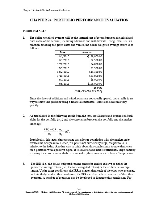
CHAPTER 24: PORTFOLIO PERFORMANCE EVALUATIONPROBLEM SETS1. The dollar-weighted average will be the internal rate of return between the initial andfinal value of the account, including additions and withdrawals. Using Excel ’s XIRR function, utilizing the given dates and values, the dollar-weighted average return is as follows:26.99%=XIRR(C13:C20,B13:B20)Since the dates of additions and withdrawals are not equally spaced, there really is no way to solve this problem using a financial calculator. Excel can solve this very quickly.2.As established in the following result from the text, the Sharpe ratio depends on both alpha for the portfolio (P α) and the correlation between the portfolio and the market index (ρ):()αρσσP f PM PPE r r S -=+ Specifically, this result demonstrates that a lower correlation with the market index reduces the Sharpe ratio. Hence, if alpha is not sufficiently large, the portfolio is inferior to the index. Another way to think about this conclusion is to note that, even for a portfolio with a positive alpha, if its diversifiable risk is sufficiently large, thereby reducing the correlation with the market index, this can result in a lower Sharpe ratio. 3.The IRR (i.e., the dollar-weighted return) cannot be ranked relative to either the geometric average return (i.e., the time-weighted return) or the arithmetic average return. Under some conditions, the IRR is greater than each of the other two averages, and similarly, under other conditions, the IRR can also be less than each of the other averages. A number of scenarios can be developed to illustrate this conclusion. Forexample, consider a scenario where the rate of return each period consistentlyincreases over several time periods. If the amount invested also increases each period, and then all of the proceeds are withdrawn at the end of several periods, the IRR isgreater than either the geometric or the arithmetic average because more money isinvested at the higher rates than at the lower rates. On the other hand, if withdrawals gradually reduce the amount invested as the rate of return increases, then the IRR is less than each of the other averages. (Similar scenarios are illustrated with numerical examples in the text, where the IRR is shown to be less than the geometric average, and in Concept Check 1, where the IRR is greater than the geometric average.)4. It is not necessarily wise to shift resources to timing at the expense of securityselection. There is also tremendous potential value in security analysis. The decision as to whether to shift resources has to be made on the basis of the macro, compared to the micro, forecasting ability of the portfolio management team.5. a. Arithmetic average: r ABC = 10%; r XYZ = 10%b.Dispersion: σABC = 7.07%; σXYZ = 13.91%Stock XYZ has greater dispersion.(Note: We used 5 degrees of freedom in calculating standard deviations.)c. Geometric average:r ABC = (1.20 × 1.12 × 1.14 × 1.03 × 1.01)1/5– 1 = 0.0977 = 9.77%r XYZ = (1.30 × 1.12 × 1.18 × 1.00 × 0.90)1/5– 1 = 0.0911 = 9.11% Despite the fact that the two stocks have the same arithmetic average, thegeometric average for XYZ is less than the geometric average for ABC. Thereason for this result is the fact that the greater variance of XYZ drives thegeometric average further below the arithmetic average.d. In terms of ―forward-looking‖ statistics, the arithmetic average is thebetter estimate of expected rate of return. Therefore, if the data reflectthe probabilities of future returns, 10 percent is the expected rate ofreturn for both stocks.6. a. Time-weighted average returns are based on year-by-year rates of return:Year Return = (Capital gains + Dividend)/Price2013 − 2014 [($120 – $100) + $4]/$100 = 24.00%2014 − 2015 [($90 – $120) + $4]/$120 = –21.67%2015 − 2016 [($100 – $90) + $4]/$90 = 15.56%Arithmetic mean: (24% – 21.67% + 15.56%)/3 = 5.96%Geometric mean: (1.24 × 0.7833 × 1.1556)1/3– 1 = 0.0392 = 3.92%b.Date CashFlow Explanation1/1/13 –$300 Purchase of three shares at $100 each1/1/14 –$228 Purchase of two shares at $120 less dividend income on three shares held 1/1/15 $110 Dividends on five shares plus sale of one share at $901/1/16 $416 Dividends on four shares plus sale of four shares at $100 each-300Dollar-weighted return = Internal rate of return = –0.1607%(CF 0 = -$300; CF 1 = -$228; CF 2 = $110; CF 3 = $416; Solve for IRR = 16.07%.)7.Time Cash Flow Holding Period Return0 3×(–$90) = –$2701 $100 (100–90)/90 = 11.11%2 $100 0%3 $100 0%a. Time-weighted geometric average rate of return =(1.1111 × 1.0 × 1.0)1/3– 1 = 0.0357 = 3.57%b. Time-weighted arithmetic average rate of return = (11.11% + 0 + 0)/3 = 3.70%The arithmetic average is always greater than or equal to the geometric average;the greater the dispersion, the greater the difference.c. Dollar-weighted average rate of return = IRR = 5.46%[Using a financial calculator, enter: n = 3, PV = –270, FV = 0, PMT = 100. Thencompute the interest rate, or use the CF0=−300, CF1=100, F1=3, then computeIRR]. The IRR exceeds the other averages because the investment fund was thelargest when the highest return occurred.8. a.The alphas for the two portfolios are:αA = 12% – [5% + 0.7 × (13% – 5%)] = 1.4% αB = 16% – [5% + 1.4 × (13% – 5%)] = –0.2%Ideally, you would want to take a long position in Portfolio A and a short position in Portfolio B.b.If you will hold only one of the two portfolios, then the Sharpe measure is the appropriate criterion:.12.050.583.12A S -== .16.050.355.31B S -== Using the Sharpe criterion, Portfolio A is the preferred portfolio.9.a.Stock A Stock B (i) Alpha = regression intercept1.0%2.0% (ii)Information ratio = ασ(e )PP 0.0971 0.1047 (iii) *Sharpe measure = σP fP r r - 0.4907 0.3373(iv)†Treynor measure = βP fPr r - 8.83310.500* To compute the Sharpe measure, note that for each stock, (r P – r f ) can becomputed from the right-hand side of the regression equation, using the assumed parameters r M = 14% and r f = 6%. The standard deviation of each stock’s returns is given in the problem.† The beta to use for the Treynor measure is the slope coefficient of the regression equation presented in the problem.b.(i) If this is the only risky asset held by the investor, then Sharpe’s measure is the appropriate measure. Since the Sharpe measure is higher for Stock A, then A is the best choice.(ii) If the stock is mixed with the market index fund, then the contribution to the overall Sharpe measure is determined by the appraisal ratio; therefore, Stock B is preferred.(iii) If the stock is one of many stocks, then Treynor’s measure is the appropriate measure, and Stock B is preferred.10. We need to distinguish between market timing and security selection abilities. Theintercept of the scatter diagram is a measure of stock selection ability. If themanager tends to have a positive excess return even when the market’sperformance is merely ―neutral‖ (i.e., has zero excess return), then we concludethat the manager has on average made good stock picks. Stock selection must be the source of the positive excess returns.Timing ability is indicated by the curvature of the plotted line. Lines that become steeper as you move to the right along the horizontal axis show good timing ability.The steeper slope shows that the manager maintained higher portfolio sensitivity to market swings (i.e., a higher beta) in periods when the market performed well. This ability to choose more market-sensitive securities in anticipation of market upturns is the essence of good timing. In contrast, a declining slope as you move to the right means that the portfolio was more sensitive to the market when the market didpoorly and less sensitive when the market did well. This indicates poor timing.We can therefore classify performance for the four managers as follows:SelectionAbility Timing AbilityA. Bad GoodB. Good GoodC. Good BadD. Bad Bad11. a. Bogey: (0.60 × 2.5%) + (0.30 × 1.2%) + (0.10 × 0.5%) = 1.91%Actual: (0.70 × 2.0%) + (0.20 × 1.0%) + (0.10 × 0.5%) = 1.65Under performance: 0.26%b. Security Selection:(1) (2) (3) = (1) × (2)Market Differential Returnwithin Market(Manager – Index)Manager'sPortfolioWeightContribution toPerformanceEquity –0.5% 0.70 −0.35% Bonds –0.2 0.20 –0.04 Cash 0.0 0.10 0.00Contribution of security selection: −0.39%c. Asset Allocation:(1) (2) (3) = (1) × (2)MarketExcess Weight(Manager – Benchmark)IndexReturnContribution toPerformanceEquity 0.10% 2.5% 0.25%Bonds –0.10 1.2 –0.12Cash 0.00 0.5 0.00Contribution of asset allocation: 0.13%Summary:Security selection –0.39%Asset allocation 0.13Excess performance –0.26%12. a. Manager: (0.30 × 20%) + (0.10 × 15%) + (0.40 × 10%) + (0.20 × 5%) = 12.50%Bogey: (0.15 × 12%) + (0.30 × 15%) + (0.45 × 14%) + (0.10 × 12%) = 13.80Added value: –1.30%b. Added value from country allocation:(1) (2) (3) = (1) × (2)CountryExcess Weight(Manager – Benchmark)Index Returnminus BogeyContribution toPerformanceU.K. 0.15 −1.8% −0.27% Japan –0.20 1.2 –0.24U.S. −0.05 0.2 −0.01Germany 0.10 −1.8 −0.18Contribution of country allocation: −0.70%c. Added value from stock selection:(1) (2) (3) = (1) × (2)Country Differential Returnwithin Country(Manager – Index)Manager’sCountry weightContribution toPerformanceU.K. 0.08 0.30% 2.4% Japan 0.00 0.10 0.0 U.S. −0.04 0.40 −1.6 Germany −0.07 0.20 −1.4Contribution of stock selection: −0.6% Summary:Country allocation –0.70%Stock selection −0.60Excess performance –1.30%13. Support : A manager could be a better performer in one type of circumstance than inanother. For example, a manager who does no timing but simply maintains a high beta, will do better in up markets and worse in down markets. Therefore, we should observe performance over an entire cycle. Also, to the extent that observing amanager over an entire cycle increases the number of observations, it would improve the reliability of the measurement.Contradict : If we adequately control for exposure to the market (i.e., adjust for beta), then market performance should not affect the relative performance of individual managers. It is therefore not necessary to wait for an entire market cycle to pass before evaluating a manager.14. The use of universes of managers to evaluate relative investment performance does,to some extent, overcome statistical problems, as long as those manager groups can be made sufficiently homogeneous with respect to style.15. a. The manager’s alpha is 10% – [6% + 0.5 × (14% – 6%)] = 0b. From Black-Jensen-Scholes and others, we know that, on average, portfolioswith low beta have historically had positive alphas. (The slope of the empirical security market line is shallower than predicted by the CAPM.) Therefore, given the manager’s low beta, performance might actually be subpar despite the estimated alpha of zero.16. a. The most likely reason for a difference in ranking is due to the absence ofdiversification in Fund A. The Sharpe ratio measures excess return per unit of total risk, while the Treynor ratio measures excess return per unit of systematic risk. Since Fund A performed well on the Treynor measure and so poorly on the Sharpe Measure, it seems that the fund carries a greater amount of unsystematic risk, meaning it is not well-diversified and systematic risk is not the relevant risk measure.17. The within sector selection calculates the return according to security selection. This isdone by summing the weight of the security in the portfolio multiplied by the return of the security in the portfolio minus the return of the security in the benchmark:Large Cap Sector: 0.6(.17-.16)= 0.6%Mid Cap Sector: 0.15(.24-.26)-0.3%Small Cap Sector: 0.25(.20-.18)= 0.5%Total Within-Sector Selection = 0.6%-0.3%0.5%0.8%⨯⨯=⨯+=18. Primo Return 0.617%0.1524%0.2520%18.8%=⨯+⨯+⨯= Benchmark Return 0.516%0.426%0.118%20.2%=⨯+⨯+⨯=Primo – Benchmar k = 18.8% − 20.2% = -1.4% (Primo underperformed benchmark) To isolate the impact of Primo’s pure sector allocation decision relative to thebenchmark, multiply the weight difference between Primo and the benchmark portfolio in each sector by the benchmark sector returns:(0.60.5)(.16)(0.150.4)(.26)(0.250.1)(.18) 2.2%-⨯+-⨯+-⨯=-To isolate the impact of Primo’s pure security selection decisions relative to thebenchmark, multiply the return differences between Primo and the benchmark for each sector by Primo’s weightings :(.17.16)(.6)(.24.26)(.15)(.20.18)(.25)0.8%-⨯+-⨯+-⨯=19. Because the passively managed fund is mimicking the benchmark, the 2R of theregression should be very high (and thus probably higher than the actively managed fund).20. a. The euro appreciated while the pound depreciated. Primo had a greater stake inthe euro-denominated assets relative to the benchmark, resulting in a positive currency allocation effect. British stocks outperformed Dutch stocks resulting in a negative market allocation effect for Primo. Finally, within the Dutch and British investments, Primo outperformed with the Dutch investments and under-performed with the British investments. Since they had a greater proportion invested in Dutch stocks relative to the benchmark, we assume that they had a positive security allocation effect in total. However, this cannot be known for certain with this information. It is the best choice, however.21. a. Miranda S&P .102.02.225.02.2216.5568σ.37.44P f P r r S S ----→====b. To compute 2M measure, blend the Miranda Fund with a position in T-bills suchthat the adjusted portfolio has the same volatility as the market index. Using the data, the position in the Miranda Fund should be .44/.37 = 1.1892 and the position in T-bills should be 1 – 1.1892 = -0.1892 (assuming borrowing at the risk-free rate).The adjusted return is: *(1.1892)10.2%(.1892)2%.117511.75%P r =⨯-⨯==Calculate the difference in the adjusted Miranda Fund return and the benchmark: *211.75%(22.50%)34.25%M P M r r =-=--=[Note: The adjusted Miranda Fund is now 59.46% equity and 40.54% cash.] c.Miranda S&P .102.02.225.02.0745.245β 1.10 1.00P f P r r T T ----→====-d.22. This exercise is left to the student; answers will vary.CFA PROBLEMS1. a. Manager AStrength . Although Manager A’s one -year total return was somewhat below the international index return (–6.0 percent versus –5.0 percent), this manager apparently has some country/security return expertise. This large local market return advantage of 2.0 percent exceeds the 0.2 percent return for the international index.Weakness. Manager A has an obvious weakness in the currency management area. This manager experienced a marked currency return shortfall, with a return of –8.0 percent versus –5.2 percent for the index.Manager BStrength . Manager B’s total return exceeded that of the index, with a marke d positive increment apparent in the currency return. Manager B had a –1.0 percent currency return compared to a –5.2 percent currency return on the international index. Based on this outcome, Manager B’s strength appears to be expertise in the currency selection area.Weakness. Manager B had a marked shortfall in local market return. Therefore, Manager B appears to be weak in security/market selection ability.b.The following strategies would enable the fund to take advantage of the strengths of each of the two managers while minimizing their weaknesses. 1. Recommendation: One strategy would be to direct Manager A to make no currency bets relative to the international index and to direct Manager B to make only currency decisions, and no active country or security selection bets.Justification: This strategy would mitigate Manager A’s weakness by hedging all currency exposures into index-like weights. This would allow capture of Manager A’s country and stock selection skills while avoiding losses from poor currency management. This strategy would also mitigateα[β()]0.102[0.02 1.10(0.2250.02)].351535.15%P P f P M f r r r r =-+-=-+⨯--==Manager B’s weakness, leaving an index-like portfolio construct andcapitalizing on the apparent skill in currency management.2. Recommendation: Another strategy would be to combine the portfolios ofManager A and Manager B, with Manager A making country exposure andsecurity selection decisions and Manager B managing the currency exposurescreated by Manager A’s decisions (providing a ―currency overlay‖).Justification: This recommendation would capture the strengths of bothManager A and Manager B and would minimize their collective weaknesses.2. a. Indeed, the one year results were terrible, but one year is a poor statistical basefrom which to draw inferences. Moreover, the board of trustees had directed Karlto adopt a long-term horizon. The board specifically instructed the investmentmanager to give priority to long-term results.b. The sample of pension funds had a much larger share invested in equities thandid Alpine. Equities performed much better than bonds. Yet the trustees toldAlpine to hold down risk, investing not more than 25 percent of the plan’s assetsin common stocks. (Alpine’s beta was also somewhat defensive.) Alpine shouldnot be held responsible for an asset allocation policy dictated by the client.c. Alpine’s alpha measures its risk-adjusted performance compared to the market:α = 13.3% – [7.5% + 0.90 × (13.8% – 7.5%)] = 0.13% (actually above zero)d.Note that the last five years, and particularly the most recent year, have beenbad for bonds, the asset class that Alpine had been encouraged to hold. Withinthis asset class, however, Alpine did much better than the index fund.Moreover, despite the fact that the bond index underperformed both theactuarial return and T-bills, Alpine outperformed both. Alpine’s performancewithin each asset class has been superior on a risk-adjusted basis. Its overalldisappointing returns were due to a heavy asset allocation weighting towardsbonds which was the b oard’s, not Alpine’s, choice.e. A trustee may not care about the time-weighted return, but that return is moreindicative of the mana ger’s performance. After all, the manager has no controlover the cash inflows and outflows of the fund.3. a. Method I does nothing to separately identify the effects of market timing andsecurity selection decisions. It also uses a questionable ―neutral position,‖ thecomposition of the portfolio at the beginning of the year.b. Method II is not perfect but is the best of the three techniques. It at least attemptsto focus on market timing by examining the returns for portfolios constructedfrom bond market indexes using actual weights in various indexes versus year-average weights. The problem with this method is that the year-average weightsneed not correspond to a client’s ―neutral‖ weights . For example, what if the manager were optimistic over the entire year regarding long-term bonds? Her average weighting could reflect her optimism, and not a neutral position.c. Method III uses net purchases of bonds as a signal of bond manager optimism.But such net purchases can be motivated by withdrawals from or contributions to the fund rather than the manager’s decisions . (Note that this is an open-ended mutual fund.) Therefore, it is inappropriate to evaluate the manager based onwhether net purchases turn out to be reliable bullish or bearish signals.4. Treynor measure = 1788.1821.1-=5. Sharpe measure = (.24.08)0.888.18-=6. a. Treynor measures(106)(126)Portfolio X: 6.67S&P 500: 6.000.6 1.0--== Sharpe measures (.10.06)(.12.06)Portfolio X: 0.222S&P 500: 0.4620.18.13--== Portfolio X outperforms the market based on the Treynor measure, but underperforms based on the Sharpe measure.b. The two measures of performance are in conflict because they use differentmeasures of risk. Portfolio X has less systematic risk than the market, asmeasured by its lower beta, but more total risk (volatility), as measured by itshigher standard deviation. Therefore, the portfolio outperforms the market based on the Treynor measure but underperforms based on the Sharpe measure.7. Geometric average = (1.15 × 0.90)1/2 – 1 = 0.0173 = 1.73%8. Geometric average = (0.91 × 1.23 × 1.17)1/3 – 1 = 0.0941 = 9.41%9. Internal rate of return = 7.5% (CF 0 = -$2,000; CF 1 = $150; CF 2 = $2,150; Solve for IRR = 7.5%)10. d.11. Time-weighted average return = 1/2(1.15 1.1)112.47%⨯-=[The arithmetic mean is: 15%10%12.5%2+=]To compute dollar-weighted rate of return, cash flows are:CF0= −$500,000CF1= −$500,000CF2 = ($500,000 × 1.15 × 1.10) + ($500,000 × 1.10) = $1,182,500 Dollar-weighted rate of return = 11.71% (Solve for IRR in financial calculator).12. a. Each of these benchmarks has several deficiencies, as described below.Market index:∙A market index may exhibit survivorship bias. Firms that have gone out ofbusiness are removed from the index, resulting in a performance measure thatoverstates actual performance had the failed firms been included.∙A market index may exhibit double counting that arises because of companiesowning other companies and both being represented in the index.∙It is often difficult to exactly and continually replicate the holdings in themarket index without incurring substantial trading costs.∙The chosen index may not be an appropriate proxy for the management style ofthe managers.∙The chosen index may not represent the entire universe of securities. Forexample, the S&P 500 Index represents 65 to 70 percent of U.S. equity marketcapitalization.∙The chosen index (e.g., the S&P 500) may have a large capitalization bias.∙The chosen index may not be investable. There may be securities in the indexthat cannot be held in the portfolio.Benchmark normal portfolio:∙This is the most difficult performance measurement method to develop andcalculate.∙The normal portfolio must be continually updated, requiring substantial resources.∙Consultants and clients are concerned that managers who are involved indeveloping and calculating their benchmark portfolio may produce aneasily-beaten normal portfolio, making their performance appear better thanit actually is.Median of the manager universe:∙It can be difficult to identify a universe of managers appropriate for theinvestment style of the plan’s managers.∙Selection of a manager universe for comparison involves some, perhaps much,subjective judgment.∙Comparison with a manager universe does not take into account the risk takenin the portfolio.∙ The median of a manager universe does not represent an ―investable‖ portfolio; that is, a portfolio manager may not be able to invest in the median managerportfolio.∙ Such a benchmark may be ambiguous. The names and weights of the securities constituting the benchmark are not clearly delineated.∙ The benchmark is not constructed prior to the start of an evaluation period; it is not specified in advance.∙ A manager universe may exhibit survivorship bias; managers who have gone out of business are removed from the universe, resulting in a performance measure that overstates the actual performance had those managers been included.b. i. The Sharpe ratio is calculated by dividing the portfolio risk premium (i.e.,actual portfolio return minus the risk-free return) by the portfolio standarddeviation: Sharpe ratio = σP f Pr r - The Treynor measure is calculated by dividing the portfolio risk premium(i.e., actual portfolio return minus the risk-free return) by the portfolio beta: Treynor measure = βP fP r r -Jensen’s alpha is calculated by subtr acting the market risk premium, adjustedfor risk by the portfolio’s beta, from the actual portfolio excess return (riskpremium). It can be described as the difference in return earned by theportfolio compared to the return implied by the Capital Asset Pricing Modelor Security Market Line:α[β()]P P f P M f r r r r =-+-ii. The Sharpe ratio assumes that the relevant risk is total risk, and it measuresexcess return per unit of total risk. The Treynor measure assumes that therelevant risk is systematic risk, and it measures excess return per unit ofsystematic risk. Jensen’s alpha assumes that the relevant risk is systematicrisk, and it measures excess return at a given level of systematic risk.13. i. Incorrect. Valid benchmarks are unbiased. Median manager benchmarks,however, are subject to significant survivorship bias, which results in severaldrawbacks, including the following:∙ The performance of median manager benchmarks is biased upwards.∙ The upward bias increases with time.∙ Survivor bias introduces uncertainty with regard to manager rankings.∙ Survivor bias skews the shape of the distribution curve.ii.Incorrect. Valid benchmarks are unambiguous and can be replicated. The median manager benchmark is ambiguous because the weights of the individualsecurities in the benchmark are not known. The portfolio’s composition cannot be known before the conclusion of a measurement period because identification as a median manager can occur only after performance is measured.Valid benchmarks are also investable. The median manager benchmark is notinvestable —a manager using a median manager benchmark cannot forgo active management and simply hold the benchmark. This is a result of the fact that the weights of individual securities in the benchmark are not known.iii. The statement is correct. The median manager benchmark may be inappropriatebecause the median manager universe encompasses many investment styles and, therefore, may not be consistent with a given manager’s style.14. a. Sharpe ratio =σP f P r r - 22.1% 5.0%24.2% 5.0%: 1.02: 0.9516.8%20.2%Williamson Joyner S S --== Treynor measure =βP f P r r - 22.1% 5.0%24.2% 5.0%: 14.25: 24.001.20.8Williamson Joyner T T --== b. The difference in the rankings of Williamson and Joyner results directly from thedifference in diversification of the portfolios. Joyner has a higher Treynormeasure (24.00) and a lower Sharpe ratio (0.95) than does Williamson (14.25and 1.202, respectively), so Joyner must be less diversified than Williamson. The Treynor measure indicates that Joyner has a higher return per unit of systematic risk than does Williamson, while the Sharpe ratio indicates that Joyner has alower return per unit of total risk than does Williamson.。

CHAPTER 4: MUTUAL FUNDS AND OTHER INVESTMENTCOMPANIESPROBLEM SETS1. The unit investment trust should have lower operating expenses.Because the investment trust portfolio is fixed once the trust isestablished, it does not have to pay portfolio managers toconstantly monitor and rebalance the portfolio as perceived needsor opportunities change. Because the portfolio is fixed, the unitinvestment trust also incurs virtually no trading costs.2. a. Unit investment trusts: Diversification from large-scaleinvesting, lower transaction costs associated with large-scaletrading, low management fees, predictable portfolio composition,guaranteed low portfolio turnover rate.b. Open-end mutual funds: Diversification from large-scaleinvesting, lower transaction costs associated with large-scaletrading, professional management that may be able to takeadvantage of buy or sell opportunities as they arise, recordkeeping.c. Individual stocks and bonds: No management fee; ability tocoordinate realization of capital gains or losses withinvestors’ personal tax situation s; capability of designingportfolio to investor’s specific risk and return profile.3. Open-end funds are obligated to redeem investor's shares at netasset value and thus must keep cash or cash-equivalent securitieson hand in order to meet potential redemptions. Closed-end funds do not need the cash reserves because there are no redemptions forclosed-end funds. Investors in closed-end funds sell their shareswhen they wish to cash out.4. Balanced funds keep relatively stable proportions of funds investedin each asset class. They are meant as convenient instruments toprovide participation in a range of asset classes. Life-cycle fundsare balanced funds whose asset mix generally depends on the age of the investor. Aggressive life-cycle funds, with larger investments in equities, are marketed to younger investors, while conservative life-cycle funds, with larger investments in fixed-income securities, are designed for older investors. Asset allocation funds, in contrast, may vary the proportions invested in each asset class by large amounts as predictions of relative performance across classes vary. Asset allocation funds therefore engage in more aggressive market timing.5. Unlike an open-end fund, in which underlying shares are redeemedwhen the fund is redeemed, a closed-end fund trades as a security in the market. Thus, their prices may differ from the NAV.6. Advantages of an ETF over a mutual fund:ETFs are continuously traded and can be sold or purchased on margin.There are no capital gains tax triggers when an ETF is sold(shares are just sold from one investor to another).Investors buy from brokers, thus eliminating the cost ofdirect marketing to individual small investors. This implieslower management fees.Disadvantages of an ETF over a mutual fund:Prices can depart from NAV (unlike an open-end fund).There is a broker fee when buying and selling (unlike a no-load fund).7. The offering price includes a 6% front-end load, or salescommission, meaning that every dollar paid results in only $ going toward purchase of shares. Therefore: Offering price =06.0170.10$Load 1NAV -=-= $8. NAV = Offering price (1 –Load) = $ .95 = $9. Stock Value Held by FundA $ 7,000,000B 12,000,000C 8,000,000D 15,000,000Total $42,000,000Net asset value =000,000,4000,30$000,000,42$-= $10. Value of stocks sold and replaced = $15,000,000 Turnover rate =000,000,42$000,000,15$= , or %11. a. 40.39$000,000,5000,000,3$000,000,200$NAV =-=b. Premium (or discount) = NAVNAV ice Pr - = 40.39$40.39$36$-= –, or % The fund sells at an % discount from NAV.12. 100NAV NAV Distributions $12.10$12.50$1.500.088, or 8.8%NAV $12.50-+-+==13. a. Start-of-year price: P 0 = $ × = $End-of-year price: P 1 = $ × = $Although NAV increased by $, the price of the fund decreased by $. Rate of return =100Distributions $11.25$12.24$1.500.042, or 4.2%$12.24P P P -+-+==b. An investor holding the same securities as the fund managerwould have earned a rate of return based on the increase in the NAV of the portfolio:100NAV NAV Distributions $12.10$12.00$1.500.133, or 13.3%NAV $12.00-+-+==14. a. Empirical research indicates that past performance of mutualfunds is not highly predictive of future performance,especially for better-performing funds. While there may be some tendency for the fund to be an above average performer nextyear, it is unlikely to once again be a top 10% performer.b. On the other hand, the evidence is more suggestive of atendency for poor performance to persist. This tendency isprobably related to fund costs and turnover rates. Thus if the fund is among the poorest performers, investors should beconcerned that the poor performance will persist.15. NAV 0 = $200,000,000/10,000,000 = $20Dividends per share = $2,000,000/10,000,000 = $NAV1 is based on the 8% price gain, less the 1% 12b-1 fee: NAV1 = $20 (1 – = $Rate of return =20$20 .0$20$384.21$+-= , or %16. The excess of purchases over sales must be due to new inflows intothe fund. Therefore, $400 million of stock previously held by the fund was replaced by new holdings. So turnover is: $400/$2,200 = , or %.17. Fees paid to investment managers were: $ billion = $ millionSince the total expense ratio was % and the management fee was %, we conclude that % must be for other expenses. Therefore, other administrative expenses were: $ billion = $ million.18. As an initial approximation, your return equals the return on the shares minus the total of the expense ratio and purchase costs: 12% % 4% = %.But the precise return is less than this because the 4% load is paid up front, not at the end of the year. To purchase the shares, you would have had to invest: $20,000/(1 = $20,833. The shares increase in value from $20,000 to: $20,000 = $22,160. The rate of return is: ($22,160 $20,833)/$20,833 = %.19. Assume $1,000 investmentLoaded-Up Fund Economy Fund Yearly growth (r is 6%) (1.01.0075)r +-- (.98)(1.0025)r ⨯+- t = 1 year$1, $1, t = 3 years$1, $1, t = 10 years$1, $1,20. a. $450,000,000$10,000000$1044,000,000-= b. The redemption of 1 million shares will most likely triggercapital gains taxes which will lower the remaining portfolio by an amount greater than $10,000,000 (implying a remaining total value less than $440,000,000). The outstanding shares fall to 43 million and the NAV drops to below $10.21. Suppose you have $1,000 to invest. The initial investment in ClassA shares is $940 net of the front-end load. After four years, yourportfolio will be worth:$940 4 = $1,Class B shares allow you to invest the full $1,000, but yourinvestment performance net of 12b-1 fees will be only %, and you will pay a 1% back-end load fee if you sell after four years. Your portfolio value after four years will be:$1,000 4 = $1,After paying the back-end load fee, your portfolio value will be:$1, .99 = $1,Class B shares are the better choice if your horizon is four years.With a 15-year horizon, the Class A shares will be worth:$940 15 = $3,For the Class B shares, there is no back-end load in this casesince the horizon is greater than five years. Therefore, the value of the Class B shares will be:$1,000 15 = $3,At this longer horizon, Class B shares are no longer the betterchoice. The effect of Class B's % 12b-1 fees accumulates over time and finally overwhelms the 6% load charged to Class A investors.22. a. After two years, each dollar invested in a fund with a 4% loadand a portfolio return equal to r will grow to: $ (1 + r–2.Each dollar invested in the bank CD will grow to: $1 .If the mutual fund is to be the better investment, then theportfolio return (r) must satisfy:(1 + r–2 >(1 + r–2 >(1 + r–2 >1 + r– >1 + r >Therefore: r > = %b. If you invest for six years, then the portfolio return mustsatisfy:(1 + r–6 > =(1 + r–6 >1 + r– >r > %The cutoff rate of return is lower for the six-year investment because the “fixed cost” (the one-time front-end load) is spread over a greater number of years.c. With a 12b-1 fee instead of a front-end load, the portfoliomust earn a rate of return (r ) that satisfies:1 + r – – >In this case, r must exceed % regardless of the investmenthorizon.23. The turnover rate is 50%. This means that, on average, 50% of theportfolio is sold and replaced with other securities each year. Trading costs on the sell orders are % and the buy orders toreplace those securities entail another % in trading costs. Total trading costs will reduce portfolio returns by: 2 % = %24. For the bond fund, the fraction of portfolio income given up tofees is: %0.4%6.0= , or % For the equity fund, the fraction of investment earnings given up to fees is:%0.12%6.0= , or % Fees are a much higher fraction of expected earnings for the bond fund and therefore may be a more important factor in selecting the bond fund.This may help to explain why unmanaged unit investment trusts are concentrated in the fixed income market. The advantages of unit investment trusts are low turnover, low trading costs, and low management fees. This is a more important concern to bond-market investors.25. Suppose that finishing in the top half of all portfolio managers ispurely luck, and that the probability of doing so in any year is exactly ½. Then the probability that any particular manager would finish in the top half of the sample five years in a row is (½)5 = 1/32. We would then expect to find that [350 (1/32)] = 11managers finish in the top half for each of the five consecutiveyears. This is precisely what we found. Thus, we should not conclude that the consistent performance after five years is proof of skill. We would expect to find 11 managers exhibiting precisely this level of "consistency" even if performance is due solely to luck.。

CHAPTER 10: ARBITRAGE PRICING THEORY ANDMULTIFACTOR MODELS OF RISK AND RETURN PROBLEM SETS1. The revised estimate of the expected rate of return on the stock would be the oldestimate plus the sum of the products of the unexpected change in each factor times the respective sensitivity coefficient:Revised estimate = 12% + [(1 × 2%) + (0.5 × 3%)] = 15.5%Note that the IP estimate is computed as: 1 × (5% - 3%), and the IR estimate iscomputed as: 0.5 × (8% - 5%).2. The APT factors must correlate with major sources of uncertainty, i.e., sources ofuncertainty that are of concern to many investors. Researchers should investigatefactors that correlate with uncertainty in consumption and investment opportunities.GDP, the inflation rate, and interest rates are among the factors that can be expected to determine risk premiums. In particular, industrial production (IP) is a goodindicator of changes in the business cycle. Thus, IP is a candidate for a factor that is highly correlated with uncertainties that have to do with investment andconsumption opportunities in the economy.3. Any pattern of returns can be explained if we are free to choose an indefinitelylarge number of explanatory factors. If a theory of asset pricing is to have value, itmust explain returns using a reasonably limited number of explanatory variables(i.e., systematic factors such as unemployment levels, GDP, and oil prices).4. Equation 10.11 applies here:E(r p) = r f + βP1 [E(r1 ) −r f ] + βP2 [E(r2 ) – r f]We need to find the risk premium (RP) for each of the two factors:RP1 = [E(r1 ) −r f] and RP2 = [E(r2 ) −r f]In order to do so, we solve the following system of two equations with two unknowns: .31 = .06 + (1.5 ×RP1 ) + (2.0 ×RP2 ).27 = .06 + (2.2 ×RP1 ) + [(–0.2) ×RP2 ]The solution to this set of equations isRP1 = 10% and RP2 = 5%Thus, the expected return-beta relationship isE(r P) = 6% + (βP1× 10%) + (βP2× 5%)5. The expected return for portfolio F equals the risk-free rate since its beta equals 0.For portfolio A, the ratio of risk premium to beta is (12 − 6)/1.2 = 5For portfolio E, the ratio is lower at (8 – 6)/0.6 = 3.33This implies that an arbitrage opportunity exists. For instance, you can create aportfolio G with beta equal to 0.6 (the same as E’s) by combining portfolio A and portfolio F in equal weights. The expected return and beta for portfolio G are then: E(r G) = (0.5 × 12%) + (0.5 × 6%) = 9%βG = (0.5 × 1.2) + (0.5 × 0%) = 0.6Comparing portfolio G to portfolio E, G has the same beta and higher return.Therefore, an arbitrage opportunity exists by buying portfolio G and selling anequal amount of portfolio E. The profit for this arbitrage will ber G – r E =[9% + (0.6 ×F)] − [8% + (0.6 ×F)] = 1%That is, 1% of the funds (long or short) in each portfolio.6. Substituting the portfolio returns and betas in the expected return-beta relationship,we obtain two equations with two unknowns, the risk-free rate (r f) and the factor risk premium (RP):12% = r f + (1.2 ×RP)9% = r f + (0.8 ×RP)Solving these equations, we obtainr f = 3% and RP = 7.5%7. a. Shorting an equally weighted portfolio of the ten negative-alpha stocks andinvesting the proceeds in an equally-weighted portfolio of the 10 positive-alpha stocks eliminates the market exposure and creates a zero-investmentportfolio. Denoting the systematic market factor as R M, the expected dollarreturn is (noting that the expectation of nonsystematic risk, e, is zero):$1,000,000 × [0.02 + (1.0 ×R M)] − $1,000,000 × [(–0.02) + (1.0 ×R M)]= $1,000,000 × 0.04 = $40,000The sensitivity of the payoff of this portfolio to the market factor is zerobecause the exposures of the positive alpha and negative alpha stocks cancelout. (Notice that the terms involving R M sum to zero.) Thus, the systematiccomponent of total risk is also zero. The variance of the analyst’s profit is notzero, however, since this portfolio is not well diversified.For n = 20 stocks (i.e., long 10 stocks and short 10 stocks) the investor willhave a $100,000 position (either long or short) in each stock. Net marketexposure is zero, but firm-specific risk has not been fully diversified. Thevariance of dollar returns from the positions in the 20 stocks is20 × [(100,000 × 0.30)2] = 18,000,000,000The standard deviation of dollar returns is $134,164.b. If n = 50 stocks (25 stocks long and 25 stocks short), the investor will have a$40,000 position in each stock, and the variance of dollar returns is50 × [(40,000 × 0.30)2] = 7,200,000,000The standard deviation of dollar returns is $84,853.Similarly, if n = 100 stocks (50 stocks long and 50 stocks short), the investorwill have a $20,000 position in each stock, and the variance of dollar returns is100 × [(20,000 × 0.30)2] = 3,600,000,000The standard deviation of dollar returns is $60,000.Notice that, when the number of stocks increases by a factor of 5 (i.e., from 20 to 100), standard deviation decreases by a factor of 5= 2.23607 (from$134,164 to $60,000).8. a. )(σσβσ2222e M +=88125)208.0(σ2222=+×=A50010)200.1(σ2222=+×=B97620)202.1(σ2222=+×=Cb. If there are an infinite number of assets with identical characteristics, then awell-diversified portfolio of each type will have only systematic risk since thenonsystematic risk will approach zero with large n. Each variance is simply β2 × market variance:222Well-diversified σ256Well-diversified σ400Well-diversified σ576A B C;;;The mean will equal that of the individual (identical) stocks.c. There is no arbitrage opportunity because the well-diversified portfolios allplot on the security market line (SML). Because they are fairly priced, there isno arbitrage.9. a. A long position in a portfolio (P) composed of portfolios A and B will offer anexpected return-beta trade-off lying on a straight line between points A and B.Therefore, we can choose weights such that βP = βC but with expected returnhigher than that of portfolio C. Hence, combining P with a short position in Cwill create an arbitrage portfolio with zero investment, zero beta, and positiverate of return.b. The argument in part (a) leads to the proposition that the coefficient of β2must be zero in order to preclude arbitrage opportunities.10. a. E(r) = 6% + (1.2 × 6%) + (0.5 × 8%) + (0.3 × 3%) = 18.1%b.Surprises in the macroeconomic factors will result in surprises in the return ofthe stock:Unexpected return from macro factors =[1.2 × (4% – 5%)] + [0.5 × (6% – 3%)] + [0.3 × (0% – 2%)] = –0.3%E(r) =18.1% − 0.3% = 17.8%11. The APT required (i.e., equilibrium) rate of return on the stock based on r f and thefactor betas isRequired E(r) = 6% + (1 × 6%) + (0.5 × 2%) + (0.75 × 4%) = 16% According to the equation for the return on the stock, the actually expected return on the stock is 15% (because the expected surprises on all factors are zero bydefinition). Because the actually expected return based on risk is less than theequilibrium return, we conclude that the stock is overpriced.12. The first two factors seem promising with respect to the likely impact on the firm’scost of capital. Both are macro factors that would elicit hedging demands acrossbroad sectors of investors. The third factor, while important to Pork Products, is a poor choice for a multifactor SML because the price of hogs is of minor importance to most investors and is therefore highly unlikely to be a priced risk factor. Betterchoices would focus on variables that investors in aggregate might find moreimportant to their welfare. Examples include: inflation uncertainty, short-terminterest-rate risk, energy price risk, or exchange rate risk. The important point here is that, in specifying a multifactor SML, we not confuse risk factors that are important toa particular investor with factors that are important to investors in general; only the latter are likely to command a risk premium in the capital markets.13. The formula is ()0.04 1.250.08 1.50.02.1717%E r =+×+×==14. If 4%f r = and based on the sensitivities to real GDP (0.75) and inflation (1.25),McCracken would calculate the expected return for the Orb Large Cap Fund to be:()0.040.750.08 1.250.02.040.0858.5% above the risk free rate E r =+×+×=+=Therefore, Kwon’s fundamental analysis estimate is congruent with McCracken’sAPT estimate. If we assume that both Kwon and McCracken’s estimates on the return of Orb’s Large Cap Fund are accurate, then no arbitrage profit is possible.15. In order to eliminate inflation, the following three equations must be solvedsimultaneously, where the GDP sensitivity will equal 1 in the first equation,inflation sensitivity will equal 0 in the second equation and the sum of the weights must equal 1 in the third equation.1.1.250.75 1.012.1.5 1.25 2.003.1wx wy wz wz wy wz wx wy wz ++=++=++=Here, x represents Orb’s High Growth Fund, y represents Large Cap Fund and z represents Utility Fund. Using algebraic manipulation will yield wx = wy = 1.6 and wz = -2.2.16. Since retirees living off a steady income would be hurt by inflation, this portfoliowould not be appropriate for them. Retirees would want a portfolio with a return positively correlated with inflation to preserve value, and less correlated with the variable growth of GDP. Thus, Stiles is wrong. McCracken is correct in that supply side macroeconomic policies are generally designed to increase output at aminimum of inflationary pressure. Increased output would mean higher GDP, which in turn would increase returns of a fund positively correlated with GDP.17. The maximum residual variance is tied to the number of securities (n ) in theportfolio because, as we increase the number of securities, we are more likely to encounter securities with larger residual variances. The starting point is todetermine the practical limit on the portfolio residual standard deviation, σ(e P ), that still qualifies as a well-diversified portfolio. A reasonable approach is to compareσ2(e P) to the market variance, or equivalently, to compare σ(e P) to the market standard deviation. Suppose we do not allow σ(e P) to exceed pσM, where p is a small decimal fraction, for example, 0.05; then, the smaller the value we choose for p, the more stringent our criterion for defining how diversified a well-diversified portfolio must be.Now construct a portfolio of n securities with weights w1, w2,…,w n, so that Σw i =1. The portfolio residual variance is σ2(e P) = Σw12σ2(e i)To meet our practical definition of sufficiently diversified, we require this residual variance to be less than (pσM)2. A sure and simple way to proceed is to assume the worst, that is, assume that the residual variance of each security is the highest possible value allowed under the assumptions of the problem: σ2(e i) = nσ2MIn that case σ2(e P) = Σw i2 nσM2Now apply the constraint: Σw i2 nσM2 ≤ (pσM)2This requires that: nΣw i2 ≤ p2Or, equivalently, that: Σw i2 ≤ p2/nA relatively easy way to generate a set of well-diversified portfolios is to use portfolio weights that follow a geometric progression, since the computations then become relatively straightforward. Choose w1 and a common factor q for the geometric progression such that q < 1. Therefore, the weight on each stock is a fraction q of the weight on the previous stock in the series. Then the sum of n terms is:Σw i= w1(1– q n)/(1– q) = 1or: w1 = (1– q)/(1– q n)The sum of the n squared weights is similarly obtained from w12 and a common geometric progression factor of q2. ThereforeΣw i2 = w12(1– q2n)/(1– q 2)Substituting for w1 from above, we obtainΣw i2 = [(1– q)2/(1– q n)2] × [(1– q2n)/(1– q 2)]For sufficient diversification, we choose q so that Σw i2 ≤ p2/nFor example, continue to assume that p = 0.05 and n = 1,000. If we chooseq = 0.9973, then we will satisfy the required condition. At this value for q w1 = 0.0029 and w n = 0.0029 × 0.99731,000In this case, w1 is about 15 times w n. Despite this significant departure from equal weighting, this portfolio is nevertheless well diversified. Any value of q between0.9973 and 1.0 results in a well-diversified portfolio. As q gets closer to 1, theportfolio approaches equal weighting.18. a. Assume a single-factor economy, with a factor risk premium E M and a (large)set of well-diversified portfolios with beta βP. Suppose we create a portfolio Zby allocating the portion w to portfolio P and (1 – w) to the market portfolioM. The rate of return on portfolio Z is:R Z = (w × R P) + [(1 – w) × R M]Portfolio Z is riskless if we choose w so that βZ = 0. This requires that:βZ = (w × βP) + [(1 – w) × 1] = 0 ⇒w = 1/(1 – βP) and (1 – w) = –βP/(1 – βP)Substitute this value for w in the expression for R Z:R Z = {[1/(1 – βP)] × R P} – {[βP/(1 – βP)] × R M}Since βZ = 0, then, in order to avoid arbitrage, R Z must be zero.This implies that: R P = βP × R MTaking expectations we have:E P = βP × E MThis is the SML for well-diversified portfolios.b. The same argument can be used to show that, in a three-factor model withfactor risk premiums E M, E1 and E2, in order to avoid arbitrage, we must have:E P = (βPM × E M) + (βP1 × E1) + (βP2 × E2)This is the SML for a three-factor economy.19. a. The Fama-French (FF) three-factor model holds that one of the factors drivingreturns is firm size. An index with returns highly correlated with firm size (i.e.,firm capitalization) that captures this factor is SMB (small minus big), thereturn for a portfolio of small stocks in excess of the return for a portfolio oflarge stocks. The returns for a small firm will be positively correlated withSMB. Moreover, the smaller the firm, the greater its residual from the othertwo factors, the market portfolio and the HML portfolio, which is the returnfor a portfolio of high book-to-market stocks in excess of the return for aportfolio of low book-to-market stocks. Hence, the ratio of the variance of thisresidual to the variance of the return on SMB will be larger and, together withthe higher correlation, results in a high beta on the SMB factor.b.This question appears to point to a flaw in the FF model. The model predictsthat firm size affects average returns so that, if two firms merge into a largerfirm, then the FF model predicts lower average returns for the merged firm.However, there seems to be no reason for the merged firm to underperformthe returns of the component companies, assuming that the component firmswere unrelated and that they will now be operated independently. We mighttherefore expect that the performance of the merged firm would be the sameas the performance of a portfolio of the originally independent firms, but theFF model predicts that the increased firm size will result in lower averagereturns. Therefore, the question revolves around the behavior of returns for aportfolio of small firms, compared to the return for larger firms that resultfrom merging those small firms into larger ones. Had past mergers of smallfirms into larger firms resulted, on average, in no change in the resultantlarger firms’ stock return characteristics (compared to the portfolio of stocksof the merged firms), the size factor in the FF model would have failed.Perhaps the reason the size factor seems to help explain stock returns is that,when small firms become large, the characteristics of their fortunes (andhence their stock returns) change in a significant way. Put differently, stocksof large firms that result from a merger of smaller firms appear empirically tobehave differently from portfolios of the smaller component firms.Specifically, the FF model predicts that the large firm will have a smaller riskpremium. Notice that this development is not necessarily a bad thing for thestockholders of the smaller firms that merge. The lower risk premium may bedue, in part, to the increase in value of the larger firm relative to the mergedfirms.CFA PROBLEMS1. a. This statement is incorrect. The CAPM requires a mean-variance efficientmarket portfolio, but APT does not.b.This statement is incorrect. The CAPM assumes normally distributed securityreturns, but APT does not.c. This statement is correct.2. b. Since portfolio X has β = 1.0, then X is the market portfolio and E(R M) =16%.Using E(R M ) = 16% and r f = 8%, the expected return for portfolio Y is notconsistent.3. d.4. c.5. d.6. c. Investors will take on as large a position as possible only if the mispricingopportunity is an arbitrage. Otherwise, considerations of risk anddiversification will limit the position they attempt to take in the mispricedsecurity.7. d.8. d.。

证券投资学10 上市公司分析在证券投资学中，对上市公司进行分析是非常重要的一项工作。

通过对上市公司的分析，投资者可以了解公司的财务状况、经营状况以及市场竞争力，从而做出明智的投资决策。

本文将探讨上市公司分析的方法和关键指标。

一、财务分析财务分析是分析上市公司的重要手段之一。

投资者通过对公司财务报表的数据进行分析，可以获得关于公司经营状况的重要信息。

1.财务报表每个上市公司都会定期发布财务报表，包括资产负债表、利润表和现金流量表。

投资者可以通过对这些报表进行分析，了解公司的财务状况。

2.关键指标在财务分析中，有一些关键指标可以帮助投资者评估上市公司的财务状况。

例如，净利润率、营业利润率、总资产周转率等指标可以帮助投资者了解公司的盈利能力和经营效率。

二、行业分析行业分析是分析上市公司的另一个重要手段。

投资者通过对所在行业的分析，可以了解行业的发展趋势和竞争状况，从而判断公司的竞争力。

1.行业发展趋势投资者可以通过研究行业的相关数据和报告，了解行业的发展趋势。

例如，市场规模、增长率和竞争格局等指标可以帮助投资者评估行业的前景。

2.竞争分析了解行业内其他公司的竞争状况对于分析上市公司非常重要。

投资者可以研究竞争对手的财务报表和经营策略，了解其优势和劣势。

三、管理层分析上市公司的管理层对公司的发展和业绩起着至关重要的作用。

因此，分析管理层的能力和经验也是分析上市公司的重要一环。

1.管理团队投资者可以通过研究公司的管理团队，了解他们的背景和经验。

具有丰富经验和专业能力的管理团队通常可以带领公司取得良好的业绩。

2.公司战略了解公司的战略规划对于分析上市公司非常重要。

投资者可以研究公司的公告和年报，了解公司的战略目标和计划。

四、风险分析投资者在分析上市公司时，还需要对公司面临的风险进行评估。

风险分析可以帮助投资者了解可能对公司业绩产生负面影响的因素。

1.市场风险市场风险是指市场环境的变化可能对公司业绩产生的影响。

CHAPTER 14: BOND PRICES AND YIELDSPROBLEM SETS1. a. Catastrophe bond—A bond that allows the issuer to transfer“catastrophe risk” from the firm to the capital markets. Investors inthese bonds receive a compensation for taking on the risk in the form ofhigher coupon rates. In the event of a catastrophe, the bondholders willreceive only part or perhaps none of the principal payment due to themat maturity. Disaster can be defined by total insured losses or by criteriasuch as wind speed in a hurricane or Richter level in an earthquake.b. Eurobond—A bond that is denominated in one currency, usually thatof the issuer, but sold in other national markets.c. Zero-coupon bond—A bond that makes no coupon payments. Investorsreceive par value at the maturity date but receive no interest paymentsuntil then. These bonds are issued at prices below par value, and theinvestor’s return comes from the difference between issue price and thepayment of par value at maturity (capital gain).d. Samurai bond—Yen-dominated bonds sold in Japan by non-Japaneseissuers.e. Junk bond—A bond with a low credit rating due to its high default risk;also known as high-yield bonds.f. Convertible bond—A bond that gives the bondholders an option toexchange the bond for a specified number of shares of common stock ofthe firm.g. Serial bonds—Bonds issued with staggered maturity dates. As bondsmature sequentially, the principal repayment burden for the firm isspread over time.h. Equipment obligation bond—A collateralized bond for which thecollateral is equipment owned by the firm. If the firm defaults on thebond, the bondholders would receive the equipment.i. Original issue discount bond—A bond issued at a discount to the facevalue.j. Indexed bond— A bond that makes payments that are tied to ageneral price index or the price of a particular commodity.k. Callable bond—A bond that gives the issuer the option to repurchase the bond at a specified call price before the maturity date.l. Puttable bond —A bond that gives the bondholder the option to sell back the bond at a specified put price before the maturity date.2. The bond callable at 105 should sell at a lower price because the call provision is more valuable to the firm. Therefore, its yield to maturity should be higher.3.Zero coupon bonds provide no coupons to be reinvested. Therefore, the investor's proceeds from the bond are independent of the rate at which coupons could be reinvested (if they were paid). There is no reinvestment rate uncertainty with zeros.4.A bond’s coupon interest payments and principal repayment are not affected by changes in market rates. Consequently, if market ratesincrease, bond investors in the secondary markets are not willing to pay as much for a claim on a gi ven bond’s fixed interest and principalpayments as they would if market rates were lower. This relationship is apparent from the inverse relationship between interest rates and present value. An increase in the discount rate (i.e., the market rate. decreases the present value of the future cash flows. 5. Annual coupon rate: 4.80% $48 Coupon paymentsCurrent yield:$48 4.95%$970⎛⎫= ⎪⎝⎭6. a.Effective annual rate for 3-month T-bill:%0.10100.0102412.11645,97000,10044==-=-⎪⎭⎫ ⎝⎛b. Effective annual interest rate for coupon bond paying 5% semiannually:(1.05.2—1 = 0.1025 or 10.25%Therefore the coupon bond has the higher effective annual interest rate. 7.The effective annual yield on the semiannual coupon bonds is 8.16%. If the annual coupon bonds are to sell at par they must offer the same yield, which requires an annual coupon rate of 8.16%.8. The bond price will be lower. As time passes, the bond price, which isnow above par value, will approach par.9. Yield to maturity: Using a financial calculator, enter the following:n = 3; PV = -953.10; FV = 1000; PMT = 80; COMP iThis results in: YTM = 9.88%Realized compound yield: First, find the future value (FV. of reinvestedcoupons and principal:FV = ($80 * 1.10 *1.12. + ($80 * 1.12. + $1,080 = $1,268.16Then find the rate (y realized . that makes the FV of the purchase price equal to $1,268.16:$953.10 ⨯ (1 + y realized .3 = $1,268.16 ⇒y realized = 9.99% or approximately 10% Using a financial calculator, enter the following: N = 3; PV = -953.10; FV =1,268.16; PMT = 0; COMP I. Answer is 9.99%.10.a. Zero coupon 8%10% couponcouponCurrent prices $463.19 $1,000.00 $1,134.20b. Price 1 year from now $500.25 $1,000.00 $1,124.94Price increase $ 37.06 $ 0.00 − $ 9.26Coupon income $ 0.00 $ 80.00 $100.00Pretax income $ 37.06 $ 80.00 $ 90.74Pretax rate of return 8.00% 8.00% 8.00%Taxes* $ 11.12 $ 24.00 $ 28.15After-tax income $ 25.94 $ 56.00 $ 62.59After-tax rate of return 5.60% 5.60% 5.52%c. Price 1 year from now $543.93 $1,065.15 $1,195.46Price increase $ 80.74 $ 65.15 $ 61.26Coupon income $ 0.00 $ 80.00 $100.00Pretax income $ 80.74 $145.15 $161.26Pretax rate of return 17.43% 14.52% 14.22%Taxes†$ 19.86 $ 37.03 $ 42.25After-tax income $ 60.88 $108.12 $119.01After-tax rate of return 13.14% 10.81% 10.49%* In computing taxes, we assume that the 10% coupon bond was issued at par and that the decrease in price when the bond is sold at year-end is treated as a capital loss and therefore is not treated as an offset to ordinary income.† In computing taxes for the zero coupon bond, $37.06 is taxed as ordinary income (see part (b); the remainder of the price increase is taxed as a capital gain.11. a. On a financial calculator, enter the following:n = 40; FV = 1000; PV = –950; PMT = 40You will find that the yield to maturity on a semiannual basis is 4.26%.This implies a bond equivalent yield to maturity equal to: 4.26% * 2 =8.52%Effective annual yield to maturity = (1.0426)2– 1 = 0.0870 = 8.70%b. Since the bond is selling at par, the yield to maturity on a semiannualbasis is the same as the semiannual coupon rate, i.e., 4%. The bondequivalent yield to maturity is 8%.Effective annual yield to maturity = (1.04)2– 1 = 0.0816 = 8.16%c. Keeping other inputs unchanged but setting PV = –1050, we find abond equivalent yield to maturity of 7.52%, or 3.76% on a semiannualbasis.Effective annual yield to maturity = (1.0376)2– 1 = 0.0766 = 7.66%12. Since the bond payments are now made annually instead of semiannually,the bond equivalent yield to maturity is the same as the effective annual yield to maturity. [On a financial calculator, n = 20; FV = 1000; PV = –price; PMT = 80]The resulting yields for the three bonds are:Bond Price Bond Equivalent Yield= Effective Annual Yield$950 8.53%1,000 8.001,050 7.51The yields computed in this case are lower than the yields calculatedwith semiannual payments. All else equal, bonds with annual payments are less attractive to investors because more time elapses beforepayments are received. If the bond price is the same with annualpayments, then the bond's yield to maturity is lower.13.Price Maturity(years.BondEquivalentYTM$400.00 20.00 4.688% 500.00 20.00 3.526 500.00 10.00 7.177385.54 10.00 10.000 463.19 10.00 8.000 400.00 11.91 8.00014. a. The bond pays $50 every 6 months. The current price is:[$50 × Annuity factor (4%, 6)] + [$1,000 × PV factor (4%, 6)] = $1,052.42 Alternatively, PMT = $50; FV = $1,000; I = 4; N = 6. Solve for PV = $1,052.42.If the market interest rate remains 4% per half year, price six months from now is:[$50 × Annuity factor (4%, 5)] + [$1,000 × PV factor (4%, 5)] = $1,044.52Alternatively, PMT = $50; FV = $1,000; I = 4; N = 5. Solve for PV = $1,044.52.b. Rate of return $50($1,044.52$1,052.42)$50$7.904.0%$1,052.42$1,052.42+--===15.The reported bond price is: $1,001.250However, 15 days have passed since the last semiannual coupon was paid, so:Accrued interest = $35 * (15/182) = $2.885The invoice price is the reported price plus accrued interest: $1,004.1416. If the yield to maturity is greater than the current yield, then the bond offers the prospect of price appreciation as it approaches its maturity date. Therefore, the bond must be selling below par value.17. The coupon rate is less than 9%. If coupon divided by price equals 9%, and price is less than par, then price divided by par is less than 9%.18.Time Inflation in YearJust EndedPar Value Coupon Payment Principal Repayment 0 $1,000.001 2% 1,020.00 $40.80 $ 0.002 3% $1,050.60 $42.02 $ 0.00 31%$1,061.11$42.44$1,061.11The nominal rate of return and real rate of return on the bond in each year are computed as follows:Nominal rate of return = interest + price appreciationinitial priceReal rate of return = 1 + nominal return1 + inflation - 1Second YearThird YearNominal return 071196.0020,1$60.30$02.42$=+050400.060.050,1$51.10$44.42$=+Real return%0.4040.0103.1071196.1==- %0.4040.0101.1050400.1==- The real rate of return in each year is precisely the 4% real yield on the bond.19.The price schedule is as follows: Year Remaining Maturity (T).Constant Yield Value $1,000/(1.08)TImputed Interest (increase inconstant yield value)0 (now) 20 years$214.551 19 231.71 $17.162 18 250.25 18.54 19 1 925.93 201,000.0074.0720.The bond is issued at a price of $800. Therefore, its yield to maturity is: 6.8245%Therefore, using the constant yield method, we find that the price in one year (when maturity falls to 9 years) will be (at an unchanged yield. $814.60, representing an increase of $14.60. Total taxable income is: $40.00 + $14.60 = $54.6021. a. The bond sells for $1,124.72 based on the 3.5% yield to maturity .[n = 60; i = 3.5; FV = 1000; PMT = 40]Therefore, yield to call is 3.368% semiannually, 6.736% annually. [n = 10 semiannual periods; PV = –1124.72; FV = 1100; PMT = 40]b. If the call price were $1,050, we would set FV = 1,050 and redo part (a) to find that yield to call is 2.976% semiannually, 5.952% annually. With a lower call price, the yield to call is lower.c. Yield to call is 3.031% semiannually, 6.062% annually. [n = 4; PV = −1124.72; FV = 1100; PMT = 40]22. The stated yield to maturity, based on promised payments, equals 16.075%.[n = 10; PV = –900; FV = 1000; PMT = 140]Based on expected reduced coupon payments of $70 annually, theexpected yield to maturity is 8.526%.23. The bond is selling at par value. Its yield to maturity equals the couponrate, 10%. If the first-year coupon is reinvested at an interest rate of rpercent, then total proceeds at the end of the second year will be: [$100 *(1 + r)] + $1,100Therefore, realized compound yield to maturity is a function of r, as shown in the following table:8% $1,208 1208/1000 – 1 = 0.0991 = 9.91%10% $1,210 1210/1000 – 1 = 0.1000 = 10.00%12% $1,212 1212/1000 – 1 = 0.1009 = 10.09%24. April 15 is midway through the semiannual coupon period. Therefore,the invoice price will be higher than the stated ask price by an amountequal to one-half of the semiannual coupon. The ask price is 101.25percent of par, so the invoice price is:$1,012.50 + (½*$50) = $1,037.5025. Factors that might make the ABC debt more attractive to investors,therefore justifying a lower coupon rate and yield to maturity, are:i. The ABC debt is a larger issue and therefore may sell with greaterliquidity.ii. An option to extend the term from 10 years to 20 years is favorable ifinterest rates 10 years from now are lower than today’s interest rates. Incontrast, if interest rates increase, the investor can present the bond forpayment and reinvest the money for a higher return.iii. In the event of trouble, the ABC debt is a more senior claim. It hasmore underlying security in the form of a first claim against realproperty.iv. The call feature on the XYZ bonds makes the ABC bonds relativelymore attractive since ABC bonds cannot be called from the investor.v. The XYZ bond has a sinking fund requiring XYZ to retire part of theissue each year. Since most sinking funds give the firm the option toretire this amount at the lower of par or market value, the sinking fundcan be detrimental for bondholders.26. A. If an investor believes the firm’s credit prospects are poor in the nearterm and wishes to capitalize on this, the investor should buy a creditdefault swap. Although a short sale of a bond could accomplish the same objective, liquidity is often greater in the swap market than it is in theunderlying cash market. The investor could pick a swap with a maturitysimilar to the expected time horizon of the credit risk. By buying theswap, the investor would receive compensation if the bond experiencesan increase in credit risk.27. a. When credit risk increases, credit default swaps increase in valuebecause the protection they provide is more valuable. Credit defaultswaps do not provide protection against interest rate risk however.28. a. An increase in the firm’s times interest-earned ratio decreases thedefault risk of the firm→increases the bond’s price → decreases the YTM.b. An increase in the issuing firm’s debt-equity ratio increases thedefault risk of the firm → decreases the bond’s price → increases YTM.c. An increase in the issuing firm’s quick ratio increases short-runliquidity, → implying a decrease in default risk of the firm → increasesthe bond’s price → decreases YTM.29. a. The floating rate note pays a coupon that adjusts to market levels.Therefore, it will not experience dramatic price changes as marketyields fluctuate. The fixed rate note will therefore have a greater pricerange.b. Floating rate notes may not sell at par for any of several reasons:(i) The yield spread between one-year Treasury bills and othermoney market instruments of comparable maturity could be wider(or narrower. than when the bond was issued.(ii) The credit standing of the firm may have eroded (or improved.relative to Treasury securities, which have no credit risk.Therefore, the 2% premium would become insufficient to sustainthe issue at par.(iii) The coupon increases are implemented with a lag, i.e., onceevery year. During a period of changing interest rates, even thisbrief lag will be reflected in the price of the security.c. The risk of call is low. Because the bond will almost surely not sell for much above par value (given its adjustable coupon rate), it is unlikely that the bond will ever be called.d. The fixed-rate note currently sells at only 88% of the call price, so that yield to maturity is greater than the coupon rate. Call risk iscurrently low, since yields would need to fall substantially for the firm to use its option to call the bond.e. The 9% coupon notes currently have a remaining maturity of 15 years and sell at a yield to maturity of 9.9%. This is the coupon rate thatwould be needed for a newly issued 15-year maturity bond to sell at par.f. Because the floating rate note pays a variable stream of interestpayments to maturity, the effective maturity for comparative purposes with other debt securities is closer to the next coupon reset date than the final maturity date. Therefore, yield-to-maturity is anindeterminable calculation for a floating rate note, with “yield -to-recoupon date” a more meaningful measure of return.30. a. The yield to maturity on the par bond equals its coupon rate, 8.75%.All else equal, the 4% coupon bond would be more attractive because its coupon rate is far below current market yields, and its price is far below the call price. Therefore, if yields fall, capital gains on the bond will not be limited by the call price. In contrast, the 8¾% coupon bond canincrease in value to at most $1,050, offering a maximum possible gain of only 0.5%. The disadvantage of the 8¾% coupon bond, in terms ofvulnerability to being called, shows up in its higher promised yield to maturity.b. If an investor expects yields to fall substantially, the 4% bond offers a greater expected return.c. Implicit call protection is offered in the sense that any likely fallin yields would not be nearly enough to make the firm considercalling the bond. In this sense, the call feature is almost irrelevant.31. a. Initial price P 0 = $705.46 [n = 20; PMT = 50; FV = 1000; i = 8]Next year's price P 1 = $793.29 [n = 19; PMT = 50; FV = 1000; i = 7] HPR %54.191954.046.705$)46.705$29.793($50$==-+=b. Using OID tax rules, the cost basis and imputed interest under theconstant yield method are obtained by discounting bond payments at the original 8% yield and simply reducing maturity by one year at a time: Constant yield prices (compare these to actual prices to compute capital gains.: P 0 = $705.46P 1 = $711.89 ⇒ implicit interest over first year = $6.43P 2 = $718.84 ⇒ implicit interest over second year = $6.95Tax on explicit interest plus implicit interest in first year =0.40*($50 + $6.43) = $22.57Capital gain in first year = Actual price at 7% YTM —constant yield price =$793.29—$711.89 = $81.40Tax on capital gain = 0.30*$81.40 = $24.42Total taxes = $22.57 + $24.42 = $46.99c. After tax HPR =%88.121288.046.705$99.46$)46.705$29.793($50$==--+d. Value of bond after two years = $798.82 [using n = 18; i = 7%; PMT = $50; FV = $1,000]Reinvested income from the coupon interest payments = $50*1.03 + $50 = $101.50Total funds after two years = $798.82 + $101.50 = $900.32Therefore, the investment of $705.46 grows to $900.32 in two years:$705.46 (1 + r )2 = $900.32 ⇒ r = 0.1297 = 12.97%e. Coupon interest received in first year: $50.00Less: tax on coupon interest 40%: – 20.00Less: tax on imputed interest (0.40*$6.43): – 2.57Net cash flow in first year: $27.43The year-1 cash flow can be invested at an after-tax rate of:3% × (1 – 0.40) = 1.8%By year 2, this investment will grow to: $27.43 × 1.018 = $27.92In two years, sell the bond for: $798.82 [n = 18; i = 7%%; PMT =$50; FV = $1,000]Less: tax on imputed interest in second year:– 2.78 [0.40 × $6.95] Add: after-tax coupon interest received in second year: + 30.00 [$50 × (1 – 0.40)]Less: Capital gains tax on(sales price – constant yield value): – 23.99 [0.30 × (798.82 – 718.84)] Add: CF from first year's coupon (reinvested):+ 27.92 [from above]Total $829.97$705.46 (1 + r)2 = $829.97 r = 0.0847 = 8.47%CFA PROBLEMS1. a. A sinking fund provision requires the early redemption of a bond issue.The provision may be for a specific number of bonds or a percentage ofthe bond issue over a specified time period. The sinking fund can retireall or a portion of an issue over the life of the issue.b. (i) Compared to a bond without a sinking fund, the sinking fundreduces the average life of the overall issue because some of thebonds are retired prior to the stated maturity.(ii) The company will make the same total principal payments overthe life of the issue, although the timing of these payments will beaffected. The total interest payments associated with the issue willbe reduced given the early redemption of principal.c. From the investor’s point of view, the key reason for demanding asinking fund is to reduce credit risk. Default risk is reduced by theorderly retirement of the issue.2. a. (i) Current yield = Coupon/Price = $70/$960 = 0.0729 = 7.29%(ii) YTM = 3.993% semiannually, or 7.986% annual bond equivalent yield.On a financial calculator, enter: n = 10; PV = –960; FV = 1000; PMT = 35Compute the interest rate.(iii) Realized compound yield is 4.166% (semiannually), or 8.332% annualbond equivalent yield. To obtain this value, first find the future value(FV) of reinvested coupons and principal. There will be six payments of$35 each, reinvested semiannually at 3% per period. On a financialcalculator, enter:PV = 0; PMT = 35; n = 6; i = 3%. Compute: FV = 226.39Three years from now, the bond will be selling at the par value of $1,000because the yield to maturity is forecast to equal the coupon rate.Therefore, total proceeds in three years will be: $226.39 + $1,000 =$1,226.39Then find the rate (y realized. that makes the FV of the purchaseprice equal to $1,226.39:$960 × (1 + y realized.6 = $1,226.39 y realized = 4.166% (semiannual.Alternatively, PV = −$960; FV = $1,226.39; N = 6; PMT = $0. Solve for I =4.16%.b. Shortcomings of each measure:(i) Current yield does not account for capital gains or losses on bondsbought at prices other than par value. It also does not account forreinvestment income on coupon payments.(ii) Yield to maturity assumes the bond is held until maturity and that all coupon income can be reinvested at a rate equal to the yield to maturity.(iii) Realized compound yield is affected by the forecast ofreinvestment rates, holding period, and yield of the bond at the endof the investor's holding period.3. a. The maturity of each bond is 10 years, and we assume that couponsare paid semiannually. Since both bonds are selling at par value, thecurrent yield for each bond is equal to its coupon rate.If the yield declines by 1% to 5% (2.5% semiannual yield., the Sentinalbond will increase in value to $107.79 [n=20; i = 2.5%; FV = 100; PMT = 3].The price of the Colina bond will increase, but only to the call price of102. The present value of scheduled payments is greater than 102, butthe call price puts a ceiling on the actual bond price.b. If rates are expected to fall, the Sentinal bond is more attractive:since it is not subject to call, its potential capital gains are greater.If rates are expected to rise, Colina is a relatively better investment. Itshigher coupon (which presumably is compensation to investors for thecall feature of the bond. will provide a higher rate of return than theSentinal bond.c. An increase in the volatility of rates will increase the value of thefirm’s option to call back the Colina bond. If rates go down, the firm can call the bond, which puts a cap on possible capital gains. So, greatervolatility makes the option to call back the bond more valuable to theissuer. This makes the bond less attractive to the investor.4. Market conversion value = Value if converted into stock = 20.83 × $28 =$583.24Conversion premium = Bond price – Market conversion value= $775.00 – $583.24 = $191.765. a. The call feature requires the firm to offer a higher coupon (or higherpromised yield to maturity) on the bond in order to compensate theinvestor for the firm's option to call back the bond at a specified priceif interest rate falls sufficiently. Investors are willing to grant thisvaluable option to the issuer, but only for a price that reflects thepossibility that the bond will be called. That price is the higherpromised yield at which they are willing to buy the bond.b. The call feature reduces the expected life of the bond. If interestrates fall substantially so that the likelihood of a call increases,investors will treat the bond as if it will "mature" and be paid off at thecall date, not at the stated maturity date. On the other hand, if ratesrise, the bond must be paid off at the maturity date, not later. Thisasymmetry means that the expected life of the bond is less than thestated maturity.c. The advantage of a callable bond is the higher coupon (and higherpromised yield to maturity) when the bond is issued. If the bond is never called, then an investor earns a higher realized compound yield on acallable bond issued at par than a noncallable bond issued at par on the same date. The disadvantage of the callable bond is the risk of call. Ifrates fall and the bond is called, then the investor receives the call price and then has to reinvest the proceeds at interest rates that are lowerthan the yield to maturity at which the bond originally was issued. Inthis event, the firm's savings in interest payments is the investor's loss.6. a. (iii)b. (iii) The yield to maturity on the callable bond must compensatethe investor for the risk of call.Choice (i) is wrong because, although the owner of a callablebond receives a premium plus the principal in the event of a call,the interest rate at which he can reinvest will be low. The lowinterest rate that makes it profitable for the issuer to call thebond also makes it a bad deal f or the bond’s holder.Choice (ii) is wrong because a bond is more apt to be called wheninterest rates are low. Only if rates are low will there be aninterest saving for the issuer.c. (iii)d. (ii)。