投资学第10版习题答案

（完整版）投资学第10版习题答案05CHAPTER 5: RISK, RETURN, AND THE HISTORICALRECORDPROBLEM SETS1. The Fisher equation predicts that the nominal rate will equal the equilibriumreal rate plus the expected inflation rate. Hence, if the inflation rate increasesfrom 3% to 5% while there is no change in the real rate, then the nominal ratewill increase by 2%. On the other hand, it is possible that an increase in theexpected inflation rate would be accompanied by a change in the real rate ofinterest. While it is conceivable that the nominal interest rate could remainconstant as the inflation rate increased, implying that the real rate decreasedas inflation increased, this is not a likely scenario.2. If we assume that the distribution of returns remains reasonably stable overthe entire history, then a longer sample period (i.e., a larger sample) increasesthe precision of the estimate of the expected rate of return; this is aconsequence of the fact that the standard error decreases as the sample sizeincreases. However, if we assume that the mean of the distribution of returnsis changing over time but we are not in a position to determine the nature ofthis change, then the expected return must be estimated from a more recentpart of the historical period. In this scenario, we must determine how far back,historically, to go in selecting the relevant sample. Here, it is likely to bedisadvantageous to use the entire data set back to 1880.3. The true statements are (c) and (e). The explanations follow.Statement (c): Let σ = the annual standard deviation of the risky investmentsand 1σ= the standard deviation of the first investment alternative over the two-year period. Then:σσ?=21Therefore, the annualized standard deviation for the first investment alternative is equal to:σσσ<=221Statement (e): The first investment alternative is more attractive to investors with lower degrees of risk aversion. The first alternative (entailing a sequence of two identically distributed and uncorrelated risky investments) is riskierthan the second alternative (the risky investment followed by a risk-freeinvestment). Therefore, the first alternative is more attractive to investors with lower degrees of risk aversion. Notice, however, that if you mistakenlybelieved that time diversification can reduce the total risk of a sequence ofrisky investments, you would have been tempted to conclude that the firstalternative is less risky and therefore more attractive to more risk-averseinvestors. This is clearly not the case; the two-year standard deviation of thefirst alternative is greater than the two-year standard deviation of the secondalternative.4. For the money market fund, your holding-period return for the next yeardepends on the level of 30-day interest rates each month when the fund rolls over maturing securities. The one-year savings deposit offers a 7.5% holding period return for the year. If you forecast that the rate on money marketinstruments will increase significantly above the current 6% yield, then themoney market fund might result in a higher HPR than the savings deposit.The 20-year Treasury bond offers a yield to maturity of 9% per year, which is 150 basis points higher than the rate on the one-year savings deposit; however, you could earn a one-year HPR much less than 7.5% on the bond if long-term interest rates increase during the year. If Treasury bond yields rise above 9%, then the price of the bond will fall, and the resulting capital loss will wipe out some or all of the 9% return you would have earned if bond yields hadremained unchanged over the course of the year.5. a. If businesses reduce their capital spending, then they are likely todecrease their demand for funds. This will shift the demand curve inFigure 5.1 to the left and reduce the equilibrium real rate of interest.b. Increased household saving will shift the supply of funds curve to theright and cause real interest rates to fall.c. Open market purchases of U.S. Treasury securities by the FederalReserve Board are equivalent to an increase in the supply of funds (ashift of the supply curve to the right). The FED buys treasuries withcash from its own account or it issues certificates which trade likecash. As a result, there is an increase in the money supply, and theequilibrium real rate of interest will fall.6. a. The “Inflation-Plus” CD is the safer investment because it guarantees thepurchasing power of the investment. Using the approximation that the realrate equals the nominal rate minus the inflation rate, the CD provides a realrate of 1.5% regardless of the inflation rate.b. The expected return depends on the expected rate of inflation over the nextyear. If the expected rate of inflation is less than 3.5% then the conventionalCD offers a higher real return than the inflation-plus CD; if the expected rateof inflation is greater than 3.5%, then the opposite is true.c. If you expect the rate of inflation to be 3% over the next year, then theconventional CD offers you an expected real rate of return of 2%, which is0.5% higher than the real rate on the inflation-protected CD. But unless youknow that inflation will be 3% with certainty, the conventional CD is alsoriskier. The question of which is the better investment then depends on yourattitude towards risk versus return. You might choose to diversify and investpart of your funds in each.d. No. We cannot assume that the entire difference between the risk-freenominal rate (on conventional CDs) of 5% and the real risk-free rate (oninflation-protected CDs) of 1.5% is the expected rate of inflation. Part of thedifference is probably a risk premium associated with the uncertaintysurrounding the real rate of return on the conventional CDs. This impliesthat the expected rate of inflation is less than 3.5% per year.7. E(r) = [0.35 × 44.5%] + [0.30 × 14.0%] + [0.35 × (–16.5%)] = 14%σ2 = [0.35 × (44.5 – 14)2] + [0.30 × (14 – 14)2] + [0.35 × (–16.5 – 14)2] = 651.175 σ = 25.52%The mean is unchanged, but the standard deviation has increased, as theprobabilities of the high and low returns have increased.8. Probability distribution of price and one-year holding period return for a 30-year U.S. Treasury bond (which will have 29 years to maturity at year-end):Economy Probability YTM Price CapitalGainCouponInterest HPRBoom 0.20 11.0% $ 74.05 -$25.95 $8.00 -17.95% Normal growth 0.50 8.0 100.00 0.00 8.00 8.00 Recession 0.30 7.0 112.28 12.28 8.00 20.289. E(q) = (0 × 0.25) + (1 × 0.25) + (2 × 0.50) = 1.25σq = [0.25 × (0 – 1.25)2 + 0.25 × (1 – 1.25)2 + 0.50 × (2 – 1.25)2]1/2 = 0.8292 10. (a) With probability 0.9544, the value of a normally distributedvariable will fall within 2 standard deviations of the mean; that is,between –40% and 80%. Simply add and subtract 2 standarddeviations to and from the mean.11. From Table 5.4, the average risk premium for the period 7/1926-9/2012 was:12.34% per year.Adding 12.34% to the 3% risk-free interest rate, the expected annual HPR for the Big/Value portfolio is: 3.00% + 12.34% = 15.34%.No. The distributions from (01/1928–06/1970) and (07/1970–12/2012) periods have distinct characteristics due to systematic shocks to the economy and subsequent government intervention. While the returns from the two periods do not differ greatly, their respective distributions tell a different story. The standard deviation for all six portfolios is larger in the first period. Skew is also positive, but negative in the second, showing a greater likelihood of higher-than-normal returns in the right tail.Kurtosis is also markedly larger in the first period.13. a%88.5,0588.070.170.080.01111or i i rn i rn rr =-=+-=-++=b. rr ≈ rn - i = 80% - 70% = 10%Clearly, the approximation gives a real HPR that is too high.14. From Table 5.2, the average real rate on T-bills has been 0.52%.a. T-bills: 0.52% real rate + 3% inflation = 3.52%b. Expected return on Big/Value:3.52% T-bill rate + 12.34% historical risk premium = 15.86%c. The risk premium on stocks remains unchanged. A premium, thedifference between two rates, is a real value, unaffected by inflation.15. Real interest rates are expected to rise. The investment activity will shiftthe demand for funds curve (in Figure 5.1) to the right. Therefore theequilibrium real interest rate will increase.16. a. Probability distribution of the HPR on the stock market and put:STOCK PUT State of theEconomyProbability Ending Price + Dividend HPR Ending Value HPR Excellent0.25 $ 131.00 31.00% $ 0.00 -100% Good0.45 114.00 14.00 $ 0.00 -100 Poor0.25 93.25 ?6.75 $ 20.25 68.75 Crash 0.05 48.00 -52.00 $ 64.00 433.33Remember that the cost of the index fund is $100 per share, and the costof the put option is $12.b. The cost of one share of the index fund plus a put option is $112. Theprobability distribution of the HPR on the portfolio is:State of the Economy Probability Ending Price + Put + DividendHPRExcellent 0.25 $ 131.00 17.0%= (131 - 112)/112 Good 0.45 114.00 1.8= (114 - 112)/112 Poor 0.25 113.50 1.3= (113.50 - 112)/112 Crash0.05 112.00 0.0 = (112 - 112)/112 c. Buying the put option guarantees the investor a minimum HPR of 0.0% regardless of what happens to the stock's price. Thus, it offers insuranceagainst a price decline.17. The probability distribution of the dollar return on CD plus call option is:State of theEconomy Probability Ending Valueof CDEnding Valueof CallCombinedValueExcellent 0.25 $ 114.00 $16.50 $130.50Good 0.45 114.00 0.00 114.00Poor 0.25 114.00 0.00 114.00Crash 0.05 114.00 0.00 114.0018.a.Total return of the bond is (100/84.49)-1 = 0.1836. With t = 10, the annualrate on the real bond is (1 + EAR) = = 1.69%.b.With a per quarter yield of 2%, the annual yield is = 1.0824, or8.24%. The equivalent continuously compounding (cc) rate is ln(1+.0824)= .0792, or 7.92%. The risk-free rate is 3.55% with a cc rate of ln(1+.0355)= .0349, or 3.49%. The cc risk premium will equal .0792 - .0349 = .0443, or4.433%.c.The appropriate formula is ,where . Using solver or goal seek, setting thetarget cell to the known effective cc rate by changing the unknown variance(cc) rate, the equivalent standard deviation (cc) is 18.03% (excel mayyield slightly different solutions).d.The expected value of the excess return will grow by 120 months (12months over a 10-year horizon). Therefore the excess return will be 120 ×4.433% = 531.9%. The expected SD grows by the square root of timeresulting in 18.03% × = 197.5%. The resulting Sharpe ratio is531.9/197.5 = 2.6929. Normsdist (-2.6929) = .0035, or a .35% probabilityof shortfall over a 10-year horizon.CFA PROBLEMS1. The expected dollar return on the investment in equities is $18,000 (0.6 × $50,000 + 0.4×?$30,000) compared to the $5,000 expected return for T-bills. Therefore, the expected risk premium is $13,000.2. E(r) = [0.2 × (?25%)] + [0.3 × 10%] + [0.5 × 24%] =10%3. E(r X) = [0.2 × (?20%)] + [0.5 × 18%] + [0.3 × 50%] =20%E(r Y) = [0.2 × (?15%)] + [0.5 × 20%] + [0.3 × 10%] =10%4. σX2 = [0.2 × (– 20 – 20)2] + [0.5 × (18 – 20)2] + [0.3 × (50 – 20)2] = 592σX = 24.33%σY2 = [0.2 × (– 15 – 10)2] + [0.5 × (20 – 10)2] + [0.3 × (10 – 10)2] = 175σY = 13.23%5. E(r) = (0.9 × 20%) + (0.1 × 10%) =19% $1,900 in returns6. The probability that the economy will be neutral is 0.50, or 50%. Given aneutral economy, the stock will experience poor performance 30% of thetime. The probability of both poor stock performance and a neutral economy is therefore: 0.30 × 0.50 = 0.15 = 15%7. E(r) = (0.1 × 15%) + (0.6 × 13%) + (0.3 × 7%) = 11.4%。

CHAPTER 7: OPTIMAL RISKY PORTFOLIOSPROBLEM SETS1. (a) and (e). Short-term rates and labor issues are factors thatare common to all firms and therefore must be considered as market risk factors. The remaining three factors are unique to this corporation and are not a part of market risk.2. (a) and (c). After real estate is added to the portfolio, there arefour asset classes in the portfolio: stocks, bonds, cash, and real estate. Portfolio variance now includes a variance term for real estate returns and a covariance term for real estate returns with returns for each of the other three asset classes. Therefore,portfolio risk is affected by the variance (or standard deviation) of real estate returns and the correlation between real estatereturns and returns for each of the other asset classes. (Note that the correlation between real estate returns and returns for cash is most likely zero.)3. (a) Answer (a) is valid because it provides the definition of theminimum variance portfolio.4. The parameters of the opportunity set are:E (r S ) = 20%, E (r B ) = 12%, σS = 30%, σB = 15%, ρ =From the standard deviations and the correlation coefficient we generate the covariance matrix [note that (,)S B S B Cov r r ρσσ=⨯⨯]: Bonds Stocks Bonds 225 45 Stocks 45 900The minimum-variance portfolio is computed as follows:w Min (S ) =1739.0)452(22590045225)(Cov 2)(Cov 222=⨯-+-=-+-B S B S B S B ,r r ,r r σσσ w Min (B ) = 1 =The minimum variance portfolio mean and standard deviation are:E (r Min ) = × .20) + × .12) = .1339 = %σMin = 2/12222)],(Cov 2[B S B S B B S Sr r w w w w ++σσ = [ 900) + 225) + (2 45)]1/2= %5.Proportion in Stock Fund Proportionin Bond Fund ExpectedReturnStandard Deviation% % % %minimumtangencyGraph shown below.0.005.0010.0015.0020.0025.000.00 5.00 10.00 15.00 20.00 25.00 30.00Tangency PortfolioMinimum Variance PortfolioEfficient frontier of risky assetsCMLINVESTMENT OPPORTUNITY SETr f = 8.006. The above graph indicates that the optimal portfolio is thetangency portfolio with expected return approximately % andstandard deviation approximately %.7. The proportion of the optimal risky portfolio invested in the stockfund is given by:222[()][()](,)[()][()][()()](,)S f B B f S B S S f B B f SS f B f S B E r r E r r Cov r r w E r r E r r E r r E r r Cov r r σσσ-⨯--⨯=-⨯+-⨯--+-⨯[(.20.08)225][(.12.08)45]0.4516[(.20.08)225][(.12.08)900][(.20.08.12.08)45]-⨯--⨯==-⨯+-⨯--+-⨯10.45160.5484B w =-=The mean and standard deviation of the optimal risky portfolio are:E (r P ) = × .20) + × .12) = .1561 = % σp = [ 900) +225) + (2× 45)]1/2= %8. The reward-to-volatility ratio of the optimal CAL is:().1561.080.4601.1654p fpE r r σ--==9. a. If you require that your portfolio yield an expected return of14%, then you can find the corresponding standard deviation from the optimal CAL. The equation for this CAL is:()().080.4601p fC f C C PE r r E r r σσσ-=+=+If E (r C ) is equal to 14%, then the standard deviation of the portfolio is %.b. To find the proportion invested in the T-bill fund, rememberthat the mean of the complete portfolio ., 14%) is an average of the T-bill rate and the optimal combination of stocks and bonds (P ). Let y be the proportion invested in the portfolio P . The mean of any portfolio along the optimal CAL is:()(1)()[()].08(.1561.08)C f P f P f E r y r y E r r y E r r y =-⨯+⨯=+⨯-=+⨯-Setting E (r C ) = 14% we find: y = and (1 − y ) = (the proportion invested in the T-bill fund).To find the proportions invested in each of the funds, multiply times the respective proportions of stocks and bonds in the optimal risky portfolio:Proportion of stocks in complete portfolio = =Proportion of bonds in complete portfolio = =10. Using only the stock and bond funds to achieve a portfolio expectedreturn of 14%, we must find the appropriate proportion in the stock fund (w S) and the appropriate proportion in the bond fund (w B = 1 −w S) as follows:= × w S + × (1 −w S) = + × w S w S =So the proportions are 25% invested in the stock fund and 75% inthe bond fund. The standard deviation of this portfolio will be:σP = [ 900) + 225) + (2 45)]1/2 = %This is considerably greater than the standard deviation of %achieved using T-bills and the optimal portfolio.11. a.Even though it seems that gold is dominated by stocks, gold mightstill be an attractive asset to hold as a part of a portfolio. Ifthe correlation between gold and stocks is sufficiently low, goldwill be held as a component in a portfolio, specifically, theoptimal tangency portfolio.b.If the correlation between gold and stocks equals +1, then no onewould hold gold. The optimal CAL would be composed of bills andstocks only. Since the set of risk/return combinations of stocksand gold would plot as a straight line with a negative slope (seethe following graph), these combinations would be dominated bythe stock portfolio. Of course, this situation could not persist.If no one desired gold, its price would fall and its expectedrate of return would increase until it became sufficientlyattractive to include in a portfolio.12. Since Stock A and Stock B are perfectly negatively correlated, arisk-free portfolio can be created and the rate of return for thisportfolio, in equilibrium, will be the risk-free rate. To find theproportions of this portfolio [with the proportion w A invested inStock A and w B = (1 –w A) invested in Stock B], set the standarddeviation equal to zero. With perfect negative correlation, theportfolio standard deviation is:σP = Absolute value [w AσA w BσB]0 = 5 × w A− [10 (1 –w A)] w A =The expected rate of return for this risk-free portfolio is:E(r) = × 10) + × 15) = %Therefore, the risk-free rate is: %13. False. If the borrowing and lending rates are not identical, then,depending on the tastes of the individuals (that is, the shape oftheir indifference curves), borrowers and lenders could havedifferent optimal risky portfolios.14. False. The portfolio standard deviation equals the weighted averageof the component-asset standard deviations only in the special case that all assets are perfectly positively correlated. Otherwise, as the formula for portfolio standard deviation shows, the portfoliostandard deviation is less than the weighted average of thecomponent-asset standard deviations. The portfolio variance is aweighted sum of the elements in the covariance matrix, with theproducts of the portfolio proportions as weights.15. The probability distribution is:Probability Rate ofReturn100%−50Mean = [ × 100%] + [ × (-50%)] = 55%Variance = [ × (100 − 55)2] + [ × (-50 − 55)2] = 4725Standard deviation = 47251/2 = %16. σP = 30 = y× σ = 40 × y y =E(r P) = 12 + (30 − 12) = %17. The correct choice is (c). Intuitively, we note that since allstocks have the same expected rate of return and standard deviation, we choose the stock that will result in lowest risk. This is thestock that has the lowest correlation with Stock A.More formally, we note that when all stocks have the same expected rate of return, the optimal portfolio for any risk-averse investor is the global minimum variance portfolio (G). When the portfolio is restricted to Stock A and one additional stock, the objective is to find G for any pair that includes Stock A, and then select thecombination with the lowest variance. With two stocks, I and J, theformula for the weights in G is:)(1)(),(Cov 2),(Cov )(222I w J w r r r r I w Min Min J I J I J I J Min -=-+-=σσσSince all standard deviations are equal to 20%:(,)400and ()()0.5I J I J Min Min Cov r r w I w J ρσσρ====This intuitive result is an implication of a property of any efficient frontier, namely, that the covariances of the global minimum variance portfolio with all other assets on the frontier are identical and equal to its own variance. (Otherwise, additional diversification would further reduce the variance.) In this case, the standard deviation of G(I, J) reduces to:1/2()[200(1)]Min IJ G σρ=⨯+This leads to the intuitive result that the desired addition would be the stock with the lowest correlation with Stock A, which is Stock D. The optimal portfolio is equally invested in Stock A and Stock D, and the standard deviation is %.18. No, the answer to Problem 17 would not change, at least as long asinvestors are not risk lovers. Risk neutral investors would not care which portfolio they held since all portfolios have an expected return of 8%.19. Yes, the answers to Problems 17 and 18 would change. The efficientfrontier of risky assets is horizontal at 8%, so the optimal CAL runs from the risk-free rate through G. This implies risk-averse investors will just hold Treasury bills.20. Rearrange the table (converting rows to columns) and compute serialcorrelation results in the following table:Nominal RatesFor example: to compute serial correlation in decade nominalreturns for large-company stocks, we set up the following twocolumns in an Excel spreadsheet. Then, use the Excel function“CORREL” to calculate the correlation for the data.Decade Previous1930s%%1940s%%1950s%%1960s%%1970s%%1980s%%1990s%%Note that each correlation is based on only seven observations, so we cannot arrive at any statistically significant conclusions.Looking at the results, however, it appears that, with theexception of large-company stocks, there is persistent serialcorrelation. (This conclusion changes when we turn to real rates in the next problem.)21. The table for real rates (using the approximation of subtracting adecade’s average inflation from the decade’s average nominalreturn) is:Real RatesSmall Company StocksLarge Company StocksLong-TermGovernmentBondsIntermed-TermGovernmentBondsTreasuryBills 1920s1930s1940s1950s1960s1970s1980s1990sSerialCorrelationWhile the serial correlation in decade nominal returns seems to be positive, it appears that real rates are serially uncorrelated. The decade time series (although again too short for any definitiveconclusions) suggest that real rates of return are independent from decade to decade.22. The 3-year risk premium for the S&P portfolio is, the 3-year risk premium for thehedge fund portfolio is S&P 3-year standard deviation is 0. The hedge fund 3-year standard deviation is 0. S&P Sharpe ratio is = , and the hedge fund Sharpe ratio is = .23. With a ρ = 0, the optimal asset allocation is,.With these weights,EThe resulting Sharpe ratio is = . Greta has a risk aversion of A=3, Therefore, she will investyof her wealth in this risky portfolio. The resulting investment composition will be S&P: = % and Hedge: = %. The remaining 26% will be invested in the risk-free asset.24. With ρ = , the annual covariance is .25. S&P 3-year standard deviation is . The hedge fund 3-year standard deviation is . Therefore, the 3-year covariance is 0.26. With a ρ=.3, the optimal asset allocation is, .With these weights,E. The resulting Sharpe ratio is = . Notice that the higher covariance results in a poorer Sharpe ratio.Greta will investyof her wealth in this risky portfolio. The resulting investment composition will be S&P: =% and hedge: = %. The remaining % will be invested in the risk-free asset.CFA PROBLEMS1. a. Restricting the portfolio to 20 stocks, rather than 40 to 50stocks, will increase the risk of the portfolio, but it ispossible that the increase in risk will be minimal. Suppose that, for instance, the 50 stocks in a universe have the same standard deviation () and the correlations between each pair areidentical, with correlation coefficient ρ. Then, the covariance between each pair of stocks would be ρσ2, and the variance of an equally weighted portfolio would be:222ρσ1σ1σnn n P -+=The effect of the reduction in n on the second term on theright-hand side would be relatively small (since 49/50 is close to 19/20 and ρσ2 is smaller than σ2), but thedenominator of the first term would be 20 instead of 50. For example, if σ = 45% and ρ = , then the standard deviation with 50 stocks would be %, and would rise to % when only 20 stocks are held. Such an increase might be acceptable if the expected return is increased sufficiently.b. Hennessy could contain the increase in risk by making sure thathe maintains reasonable diversification among the 20 stocks that remain in his portfolio. This entails maintaining a low correlation among the remaining stocks. For example, in part (a), with ρ = , the increase in portfolio risk was minimal. As a practical matter, this means that Hennessy would have to spread his portfolio among many industries; concentrating on just a few industries would result in higher correlations among the included stocks.2. Risk reduction benefits from diversification are not a linearfunction of the number of issues in the portfolio. Rather, the incremental benefits from additional diversification are mostimportant when you are least diversified. Restricting Hennessy to 10 instead of 20 issues would increase the risk of his portfolio by a greater amount than would a reduction in the size of theportfolio from 30 to 20 stocks. In our example, restricting the number of stocks to 10 will increase the standard deviation to %. The % increase in standard deviation resulting from giving up 10 of20 stocks is greater than the % increase that results from givingup 30 of 50 stocks.3. The point is well taken because the committee should be concernedwith the volatility of the entire portfolio. Since Hennessy’sportfolio is only one of six well-diversified portfolios and issmaller than the average, the concentration in fewer issues mighthave a minimal effect on the diversification of the total fund.Hence, unleashing Hennessy to do stock picking may be advantageous.4. d. Portfolio Y cannot be efficient because it is dominated byanother portfolio. For example, Portfolio X has both higherexpected return and lower standard deviation.5. c.6. d.7. b.8. a.9. c.10. Since we do not have any information about expected returns, wefocus exclusively on reducing variability. Stocks A and C have equal standard deviations, but the correlation of Stock B with Stock C is less than that of Stock A with Stock B . Therefore, a portfoliocomposed of Stocks B and C will have lower total risk than aportfolio composed of Stocks A and B.11. Fund D represents the single best addition to complementStephenson's current portfolio, given his selection criteria. Fund D’s expected return percent) has the potential to increase theportfolio’s return somewhat. Fund D’s relatively low correlation with his current portfolio (+ indicates that Fund D will providegreater diversification benefits than any of the other alternativesexcept Fund B. The result of adding Fund D should be a portfolio with approximately the same expected return and somewhat lower volatility compared to the original portfolio.The other three funds have shortcomings in terms of expected return enhancement or volatility reduction through diversification. Fund A offers the potential for increasing the portfolio’s return but is too highly correlated to provide substantial volatility reduction benefits through diversification. Fund B provides substantial volatility reduction through diversification benefits but is expected to generate a return well below the current portfolio’s return. Fund C has the greatest potential to increase the portfolio’s return but is too highly correlated with the current portfolio to provide substantial volatility reduction benefits through diversification.12. a. Subscript OP refers to the original portfolio, ABC to thenew stock, and NP to the new portfolio.i. E(r NP) = w OP E(r OP) + w ABC E(r ABC) = + = %ii. Cov = ρOP ABC = =iii. NP = [w OP2OP2 + w ABC2ABC2 + 2 w OP w ABC(Cov OP , ABC)]1/2= [ 2 + + (2 ]1/2= % %b. Subscript OP refers to the original portfolio, GS to governmentsecurities, and NP to the new portfolio.i. E(r NP) = w OP E(r OP) + w GS E(r GS) = + = %ii. Cov = ρOP GS = 0 0 = 0iii. NP = [w OP2OP2 + w GS2GS2 + 2 w OP w GS (Cov OP , GS)]1/2= [ + 0) + (2 0)]1/2= % %c. Adding the risk-free government securities would result in alower beta for the new portfolio. The new portfolio beta will bea weighted average of the individual security betas in theportfolio; the presence of the risk-free securities would lowerthat weighted average.d. The comment is not correct. Although the respective standarddeviations and expected returns for the two securities underconsideration are equal, the covariances between each security andthe original portfolio are unknown, making it impossible to drawthe conclusion stated. For instance, if the covariances aredifferent, selecting one security over the other may result in alower standard deviation for the portfolio as a whole. In such acase, that security would be the preferred investment, assumingall other factors are equal.e. i. Grace clearly expressed the sentiment that the risk of losswas more important to her than the opportunity for return. Usingvariance (or standard deviation) as a measure of risk in her casehas a serious limitation because standard deviation does notdistinguish between positive and negative price movements.ii. Two alternative risk measures that could be used instead ofvariance are:Range of returns, which considers the highest and lowestexpected returns in the future period, with a larger rangebeing a sign of greater variability and therefore of greaterrisk.Semivariance can be used to measure expected deviations ofreturns below the mean, or some other benchmark, such as zero.Either of these measures would potentially be superior tovariance for Grace. Range of returns would help to highlightthe full spectrum of risk she is assuming, especially thedownside portion of the range about which she is so concerned.Semivariance would also be effective, because it implicitlyassumes that the investor wants to minimize the likelihood ofreturns falling below some target rate; in Grace’s case, thetarget rate would be set at zero (to protect against negativereturns).13. a. Systematic risk refers to fluctuations in asset prices causedby macroeconomic factors that are common to all risky assets;hence systematic risk is often referred to as market risk.Examples of systematic risk factors include the business cycle,inflation, monetary policy, fiscal policy, and technologicalchanges.Firm-specific risk refers to fluctuations in asset pricescaused by factors that are independent of the market, such asindustry characteristics or firm characteristics. Examples offirm-specific risk factors include litigation, patents,management, operating cash flow changes, and financial leverage.b. Trudy should explain to the client that picking only the topfive best ideas would most likely result in the client holdinga much more risky portfolio. The total risk of a portfolio, orportfolio variance, is the combination of systematic risk andfirm-specific risk.The systematic component depends on the sensitivity of theindividual assets to market movements as measured by beta.Assuming the portfolio is well diversified, the number ofassets will not affect the systematic risk component ofportfolio variance. The portfolio beta depends on theindividual security betas and the portfolio weights of those securities.On the other hand, the components of firm-specific risk (sometimes called nonsystematic risk) are not perfectly positively correlated with each other and, as more assets are added to the portfolio, those additional assets tend to reduce portfolio risk. Hence, increasing the number of securities in a portfolio reduces firm-specific risk. For example, a patent expiration for one company would not affect the othersecurities in the portfolio. An increase in oil prices islikely to cause a drop in the price of an airline stock butwill likely result in an increase in the price of an energy stock. As the number of randomly selected securities increases, the total risk (variance) of the portfolio approaches its systematic variance.。

博迪《投资学》（第10版）笔记和课后习题详解答案博迪《投资学》（第10版）笔记和课后习题详解完整版>精研学习?>无偿试用20％资料全国547所院校视频及题库全收集考研全套>视频资料>课后答案>往年真题>职称考试第一部分绪论第1章投资环境1.1复习笔记1.2课后习题详解第2章资产类别与金融工具2.1复习笔记2.2课后习题详解第3章证券是如何交易的3.1复习笔记3.2课后习题详解第4章共同基金与其他投资公司4.1复习笔记4.2课后习题详解第二部分资产组合理论与实践第5章风险与收益入门及历史回顾5.1复习笔记5.2课后习题详解第6章风险资产配置6.1复习笔记6.2课后习题详解第7章最优风险资产组合7.1复习笔记7.2课后习题详解第8章指数模型8.2课后习题详解第三部分资本市场均衡第9章资本资产定价模型9.1复习笔记9.2课后习题详解第10章套利定价理论与风险收益多因素模型10.1复习笔记10.2课后习题详解第11章有效市场假说11.1复习笔记11.2课后习题详解第12章行为金融与技术分析12.1复习笔记12.2课后习题详解第13章证券收益的实证证据13.1复习笔记13.2课后习题详解第四部分固定收益证券第14章债券的价格与收益14.1复习笔记14.2课后习题详解第15章利率的期限结构15.1复习笔记15.2课后习题详解第16章债券资产组合管理16.1复习笔记16.2课后习题详解第五部分证券分析第17章宏观经济分析与行业分析17.2课后习题详解第18章权益估值模型18.1复习笔记18.2课后习题详解第19章财务报表分析19.1复习笔记19.2课后习题详解第六部分期权、期货与其他衍生证券第20章期权市场介绍20.1复习笔记20.2课后习题详解第21章期权定价21.1复习笔记21.2课后习题详解第22章期货市场22.1复习笔记22.2课后习题详解第23章期货、互换与风险管理23.1复习笔记23.2课后习题详解第七部分应用投资组合管理第24章投资组合业绩评价24.1复习笔记24.2课后习题详解第25章投资的国际分散化25.1复习笔记25.2课后习题详解第26章对冲基金26.1复习笔记26.2课后习题详解第27章积极型投资组合管理理论27.1复习笔记27.2课后习题详解第28章投资政策与特许金融分析师协会结构28.1复习笔记28.2课后习题详解。

第三部分资本市场均衡第9章资本资产定价模型一、选择题1．如果一个股票的价值是高估的，则它应位于（）。

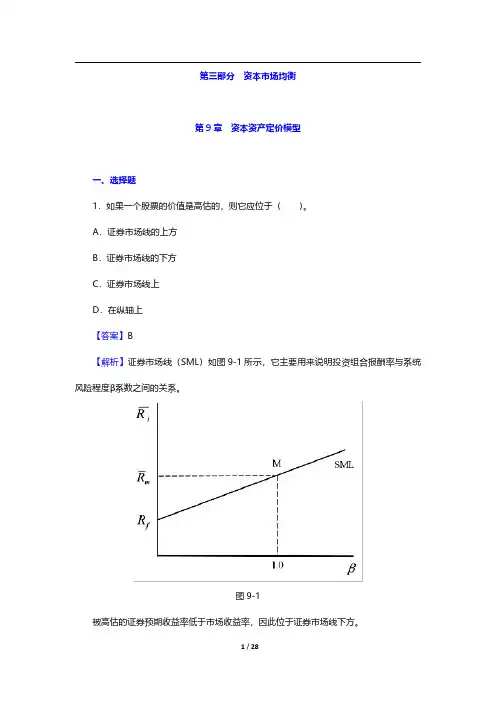
A．证券市场线的上方B．证券市场线的下方C．证券市场线上D．在纵轴上【答案】B【解析】证券市场线（SML）如图9-1所示，它主要用来说明投资组合报酬率与系统风险程度β系数之间的关系。

图9-1被高估的证券预期收益率低于市场收益率，因此位于证券市场线下方。

2．无风险利率和市场预期收益率分别是3.5%和10.5%。

根据资本资产定价模型，一只β值是1.63的证券的预期收益是（）。

A．10.12%B．14.91%C．16.56%D．18.79%【答案】B【解析】根据资本资产定价模型：E（r i）＝r f＋β[E（r M）－r f]＝3.5%＋1.63×（10.5%－3.5%）＝14.91%。

3．资本资产定价模型给出了精确预测（）的方法。

A．有效投资组合B．单一资产与风险资产组合期望收益率C．不同风险收益偏好下最优风险投资组合D．资产风险及其期望收益率之间的关系【答案】D【解析】根据资本资产定价模型，每一证券的期望收益率应等于无风险利率加上该证券由β系数测定的风险溢价。

4．假定一只股票定价合理，预期收益是15%，市场预期收益是10.5%，无风险利率是3.5%，这只股票的β值是（）。

A．1.36B．1.52C．1.64D．1.75【答案】C【解析】既然α值假定为零，证券的收益就等于CAPM设定的收益。

因此，将已知的数值代入CAPM，即15%＝[3.5%＋（10.5%－3.5%）β]，解得：β＝1.64。

5．根据CAPM模型，市场期望收益率和无风险收益率分别是0.12和0.06，β值为1.2的证券A的期望收益率是（）。

A．0.068B．0.12C．0.132D．0.142【答案】C【解析】根据资本资产定价模型，E（r i）＝r f＋[E（r M）－r f]βi＝0.06＋（0.12－0.06）×1.2＝0.132。

CHAPTER 4: MUTUAL FUNDS AND OTHER INVESTMENTCOMPANIESPROBLEM SETS1. The unit investment trust should have lower operating expenses.Because the investment trust portfolio is fixed once the trust isestablished, it does not have to pay portfolio managers toconstantly monitor and rebalance the portfolio as perceived needsor opportunities change. Because the portfolio is fixed, the unitinvestment trust also incurs virtually no trading costs.2. a. Unit investment trusts: Diversification from large-scaleinvesting, lower transaction costs associated with large-scaletrading, low management fees, predictable portfolio composition,guaranteed low portfolio turnover rate.b. Open-end mutual funds: Diversification from large-scaleinvesting, lower transaction costs associated with large-scaletrading, professional management that may be able to takeadvantage of buy or sell opportunities as they arise, recordkeeping.c. Individual stocks and bonds: No management fee; ability tocoordinate realization of capital gains or losses withinvestors’ personal tax situation s; capability of designingportfolio to investor’s specific risk and return profile.3. Open-end funds are obligated to redeem investor's shares at netasset value and thus must keep cash or cash-equivalent securitieson hand in order to meet potential redemptions. Closed-end funds do not need the cash reserves because there are no redemptions forclosed-end funds. Investors in closed-end funds sell their shareswhen they wish to cash out.4. Balanced funds keep relatively stable proportions of funds investedin each asset class. They are meant as convenient instruments toprovide participation in a range of asset classes. Life-cycle fundsare balanced funds whose asset mix generally depends on the age of the investor. Aggressive life-cycle funds, with larger investments in equities, are marketed to younger investors, while conservative life-cycle funds, with larger investments in fixed-income securities, are designed for older investors. Asset allocation funds, in contrast, may vary the proportions invested in each asset class by large amounts as predictions of relative performance across classes vary. Asset allocation funds therefore engage in more aggressive market timing.5. Unlike an open-end fund, in which underlying shares are redeemedwhen the fund is redeemed, a closed-end fund trades as a security in the market. Thus, their prices may differ from the NAV.6. Advantages of an ETF over a mutual fund:ETFs are continuously traded and can be sold or purchased on margin.There are no capital gains tax triggers when an ETF is sold(shares are just sold from one investor to another).Investors buy from brokers, thus eliminating the cost ofdirect marketing to individual small investors. This implieslower management fees.Disadvantages of an ETF over a mutual fund:Prices can depart from NAV (unlike an open-end fund).There is a broker fee when buying and selling (unlike a no-load fund).7. The offering price includes a 6% front-end load, or salescommission, meaning that every dollar paid results in only $ going toward purchase of shares. Therefore: Offering price =06.0170.10$Load 1NAV -=-= $8. NAV = Offering price (1 –Load) = $ .95 = $9. Stock Value Held by FundA $ 7,000,000B 12,000,000C 8,000,000D 15,000,000Total $42,000,000Net asset value =000,000,4000,30$000,000,42$-= $10. Value of stocks sold and replaced = $15,000,000 Turnover rate =000,000,42$000,000,15$= , or %11. a. 40.39$000,000,5000,000,3$000,000,200$NAV =-=b. Premium (or discount) = NAVNAV ice Pr - = 40.39$40.39$36$-= –, or % The fund sells at an % discount from NAV.12. 100NAV NAV Distributions $12.10$12.50$1.500.088, or 8.8%NAV $12.50-+-+==13. a. Start-of-year price: P 0 = $ × = $End-of-year price: P 1 = $ × = $Although NAV increased by $, the price of the fund decreased by $. Rate of return =100Distributions $11.25$12.24$1.500.042, or 4.2%$12.24P P P -+-+==b. An investor holding the same securities as the fund managerwould have earned a rate of return based on the increase in the NAV of the portfolio:100NAV NAV Distributions $12.10$12.00$1.500.133, or 13.3%NAV $12.00-+-+==14. a. Empirical research indicates that past performance of mutualfunds is not highly predictive of future performance,especially for better-performing funds. While there may be some tendency for the fund to be an above average performer nextyear, it is unlikely to once again be a top 10% performer.b. On the other hand, the evidence is more suggestive of atendency for poor performance to persist. This tendency isprobably related to fund costs and turnover rates. Thus if the fund is among the poorest performers, investors should beconcerned that the poor performance will persist.15. NAV 0 = $200,000,000/10,000,000 = $20Dividends per share = $2,000,000/10,000,000 = $NAV1 is based on the 8% price gain, less the 1% 12b-1 fee: NAV1 = $20 (1 – = $Rate of return =20$20 .0$20$384.21$+-= , or %16. The excess of purchases over sales must be due to new inflows intothe fund. Therefore, $400 million of stock previously held by the fund was replaced by new holdings. So turnover is: $400/$2,200 = , or %.17. Fees paid to investment managers were: $ billion = $ millionSince the total expense ratio was % and the management fee was %, we conclude that % must be for other expenses. Therefore, other administrative expenses were: $ billion = $ million.18. As an initial approximation, your return equals the return on the shares minus the total of the expense ratio and purchase costs: 12% % 4% = %.But the precise return is less than this because the 4% load is paid up front, not at the end of the year. To purchase the shares, you would have had to invest: $20,000/(1 = $20,833. The shares increase in value from $20,000 to: $20,000 = $22,160. The rate of return is: ($22,160 $20,833)/$20,833 = %.19. Assume $1,000 investmentLoaded-Up Fund Economy Fund Yearly growth (r is 6%) (1.01.0075)r +-- (.98)(1.0025)r ⨯+- t = 1 year$1, $1, t = 3 years$1, $1, t = 10 years$1, $1,20. a. $450,000,000$10,000000$1044,000,000-= b. The redemption of 1 million shares will most likely triggercapital gains taxes which will lower the remaining portfolio by an amount greater than $10,000,000 (implying a remaining total value less than $440,000,000). The outstanding shares fall to 43 million and the NAV drops to below $10.21. Suppose you have $1,000 to invest. The initial investment in ClassA shares is $940 net of the front-end load. After four years, yourportfolio will be worth:$940 4 = $1,Class B shares allow you to invest the full $1,000, but yourinvestment performance net of 12b-1 fees will be only %, and you will pay a 1% back-end load fee if you sell after four years. Your portfolio value after four years will be:$1,000 4 = $1,After paying the back-end load fee, your portfolio value will be:$1, .99 = $1,Class B shares are the better choice if your horizon is four years.With a 15-year horizon, the Class A shares will be worth:$940 15 = $3,For the Class B shares, there is no back-end load in this casesince the horizon is greater than five years. Therefore, the value of the Class B shares will be:$1,000 15 = $3,At this longer horizon, Class B shares are no longer the betterchoice. The effect of Class B's % 12b-1 fees accumulates over time and finally overwhelms the 6% load charged to Class A investors.22. a. After two years, each dollar invested in a fund with a 4% loadand a portfolio return equal to r will grow to: $ (1 + r–2.Each dollar invested in the bank CD will grow to: $1 .If the mutual fund is to be the better investment, then theportfolio return (r) must satisfy:(1 + r–2 >(1 + r–2 >(1 + r–2 >1 + r– >1 + r >Therefore: r > = %b. If you invest for six years, then the portfolio return mustsatisfy:(1 + r–6 > =(1 + r–6 >1 + r– >r > %The cutoff rate of return is lower for the six-year investment because the “fixed cost” (the one-time front-end load) is spread over a greater number of years.c. With a 12b-1 fee instead of a front-end load, the portfoliomust earn a rate of return (r ) that satisfies:1 + r – – >In this case, r must exceed % regardless of the investmenthorizon.23. The turnover rate is 50%. This means that, on average, 50% of theportfolio is sold and replaced with other securities each year. Trading costs on the sell orders are % and the buy orders toreplace those securities entail another % in trading costs. Total trading costs will reduce portfolio returns by: 2 % = %24. For the bond fund, the fraction of portfolio income given up tofees is: %0.4%6.0= , or % For the equity fund, the fraction of investment earnings given up to fees is:%0.12%6.0= , or % Fees are a much higher fraction of expected earnings for the bond fund and therefore may be a more important factor in selecting the bond fund.This may help to explain why unmanaged unit investment trusts are concentrated in the fixed income market. The advantages of unit investment trusts are low turnover, low trading costs, and low management fees. This is a more important concern to bond-market investors.25. Suppose that finishing in the top half of all portfolio managers ispurely luck, and that the probability of doing so in any year is exactly ½. Then the probability that any particular manager would finish in the top half of the sample five years in a row is (½)5 = 1/32. We would then expect to find that [350 (1/32)] = 11managers finish in the top half for each of the five consecutiveyears. This is precisely what we found. Thus, we should not conclude that the consistent performance after five years is proof of skill. We would expect to find 11 managers exhibiting precisely this level of "consistency" even if performance is due solely to luck.。

CHAPTER 8: INDEX MODELSPROBLEM SETS1. The advantage of the index model, compared to the Markowitz procedure, is thevastly reduced number of estimates required. In addition, the large number ofestimates required for the Markowitz procedure can result in large aggregateestimation errors when implementing the procedure. The disadvantage of the index model arises from the model’s assumption that return residuals are uncorrelated.This assumption will be incorrect if the index used omits a significant risk factor.2. The trade-off entailed in departing from pure indexing in favor of an activelymanaged portfolio is between the probability (or the possibility) of superiorperformance against the certainty of additional management fees.3. The answer to this question can be seen from the formulas for w0 (equation 8.20)and w* (equation 8.21). Other things held equal, w0 is smaller the greater theresidual variance of a candidate asset for inclusion in the portfolio. Further, we see that regardless of beta, when w0 decreases, so does w*. Therefore, other thingsequal, the greater the residual variance of an asset, the smaller its position in the optimal risky portfolio. That is, increased firm-specific risk reduces the extent to which an active investor will be willing to depart from an indexed portfolio.4. The total risk premium equals: ? + (? × Market risk premium). We call alpha anonmarket return premium because it is the portion of the return premium that is independent of market performance.The Sharpe ratio indicates that a higher alpha makes a security more desirable.Alpha, the numerator of the Sharpe ratio, is a fixed number that is not affected by the standard deviation of returns, the denominator of the Sharpe ratio. Hence, an increase in alpha increases the Sharpe ratio. Since the portfolio alpha is theportfolio-weighted average of the securities’ alphas, then, holding all otherparameters fixed, an increase in a security’s alpha results in an increase in theportfolio Sharpe ratio.5. a. To optimize this portfolio one would need:n = 60 estimates of means n = 60 estimates of variances770,122=-nn estimates of covariances Therefore, in total: 890,1232=+nn estimatesb.In a single index model: r i ? r f = α i + β i (r M – r f ) + e i Equivalently, using excess returns: R i = α i + β i R M + e iThe variance of the rate of return can be decomposed into the components: (l)The variance due to the common market factor: 22M i σβ(2) The variance due to firm specific unanticipated events: )(σ2i e In this model: σββ),(Cov j i j i r r = The number of parameter estimates is:n = 60 estimates of the mean E (r i )n = 60 estimates of the sensitivity coefficient β i n = 60 estimates of the firm-specific variance σ2(e i ) 1 estimate of the market mean E (r M )1 estimate of the market variance 2M σTherefore, in total, 182 estimates.The single index model reduces the total number of required estimates from 1,890 to 182. In general, the number of parameter estimates is reduced from:)23( to 232+⎪⎪⎭⎫ ⎝⎛+n n n6.a.The standard deviation of each individual stock is given by:2/1222)](β[σi M i i e σσ+=Since βA = 0.8, βB = 1.2, σ(e A ) = 30%, σ(e B ) = 40%, and σM = 22%, we get:σA = (0.82 × 222 + 302 )1/2 = 34.78% σB = (1.22 × 222 + 402 )1/2 = 47.93%b.The expected rate of return on a portfolio is the weighted average of the expected returns of the individual securities:E(r P ) = w A × E(r A ) + w B × E(r B ) + w f × r fE(r P ) = (0.30 × 13%) + (0.45 × 18%) + (0.25 × 8%) = 14% The beta of a portfolio is similarly a weighted average of the betas of the individual securities:βP = w A × βA + w B × βB + w f × β fβP = (0.30 × 0.8) + (0.45 × 1.2) + (0.25 × 0.0) = 0.78 The variance of this portfolio is:)(σβσ2222P M P P e +=σwhere 22σβM P is the systematic component and )(2P e σis the nonsystematic component. Since the residuals (e i ) are uncorrelated, the nonsystematic variance is:2222222()()()()P A A B B f f e w e w e w e σσσσ=⨯+⨯+⨯= (0.302 × 302 ) + (0.452 × 402 ) + (0.252 × 0) = 405where σ2(e A ) and σ2(e B ) are the firm-specific (nonsystematic) variances of Stocks A and B, and σ2(e f ), the nonsystematic variance of T-bills, is zero. The residual standard deviation of the portfolio is thus:σ(e P ) = (405)1/2 = 20.12% The total variance of the portfolio is then:47.699405)2278.0(σ222=+⨯=PThe total standard deviation is 26.45%.7.a.The two figures depict the stocks’ security characteri stic lines (SCL). Stock A has higher firm-specific risk because the deviations of the observations from the SCL are larger for Stock A than for Stock B. Deviations are measured by the vertical distance of each observation from the SCL.b. Beta is the slope of the SCL, which is the measure of systematic risk. The SCL for Stock B is st eeper; hence Stock B’s systematic risk is greater.c.The R 2 (or squared correlation coefficient) of the SCL is the ratio of the explained variance of the stock’s return to total variance, and the totalvariance is the sum of the explained variance plus the unexplained variance (the stock’s residual variance):)(σσβσβ222222i M i M i e R += Since the explained variance for Stock B is greater than for Stock A (theexplained variance is 22σβM B , which is greater since its beta is higher), and its residual variance 2()B e σ is smaller, its R 2 is higher than Stock A’s.d. Alpha is the intercept of the SCL with the expected return axis. Stock A has a small positive alpha whereas Stock B has a negative alpha; hence, Stock A’s alpha is larger.e. The correlation coefficient is simply the square root of R 2, so Stock B’s correlation with the market is higher.8. a.Firm-specific risk is measured by the residual standard deviation. Thus, stock A has more firm-specific risk: 10.3% > 9.1%b. Market risk is measured by beta, the slope coefficient of the regression. A has a larger beta coefficient: 1.2 > 0.8c. R 2 measures the fraction of total variance of return explained by the market return. A’s R 2 is larger than B’s: 0.576 > 0.436d.Rewriting the SCL equation in terms of total return (r ) rather than excess return (R ):()(1)A f M f A f Mr r r r r r r αβαββ-=+⨯-⇒=+⨯-+⨯The intercept is now equal to:(1)1%(1 1.2)f f r r αβ+⨯-=+⨯-Since r f = 6%, the intercept would be: 1%6%(1 1.2)1% 1.2%0.2%+-=-=-9.The standard deviation of each stock can be derived from the following equation for R 2:==2222σσβiMi iR Explained variance Total variance Therefore:%30.31σ98020.0207.0σβσ222222==⨯==A A MA AR For stock B:%28.69σ800,412.0202.1σ222==⨯=B B10. The systematic risk for A is:22220.7020196A M βσ⨯=⨯=The firm-specific risk of A (the residual variance) is the difference between A’s total risk and its systematic risk:980 – 196 = 784 The systematic risk for B is:22221.2020576B M βσ⨯=⨯=B’s firm -specific risk (residual variance) is:4,800 – 576 = 4,22411. The covariance between the returns of A and B is (since the residuals are assumedto be uncorrelated):33640020.170.0σββ)(Cov 2=⨯⨯==M B A B A ,r rThe correlation coefficient between the returns of A and B is:155.028.6930.31336σσ),(Cov ρ=⨯==B A B A AB r r12. Note that the correlation is the square root of R 2:2ρR =1/2,1/2,()0.2031.3020280()0.1269.2820480A M A MB M B M Cov r r Cov r r ρσσρσσ==⨯⨯===⨯⨯=13. For portfolio P we can compute:σP = [(0.62 × 980) + (0.42 × 4800) + (2 × 0.4 × 0.6 × 336)]1/2 = [1282.08]1/2 = 35.81% βP = (0.6 × 0.7) + (0.4 × 1.2) = 0.90958.08400)(0.901282.08σβσ)(σ22222=⨯-=-=M P P P eCov(r P ,r M ) = βP 2σM =0.90 ×400=360 This same result can also be attained using the covariances of the individual stocks with the market:Cov(r P ,r M ) = Cov(0.6r A + 0.4r B , r M ) = 0.6 × Cov(r A , r M ) + 0.4 × Cov(r B ,r M )= (0.6 × 280) + (0.4 × 480) = 36014. Note that the variance of T-bills is zero, and the covariance of T-bills with any assetis zero. Therefore, for portfolio Q:[][]%55.21)3603.05.02()4003.0()08.282,15.0(),(Cov 2σσσ2/1222/12222=⨯⨯⨯+⨯+⨯=⨯⨯⨯++=M P M P M M P P Q r r w w w w(0.50.90)(0.31)(0.200)0.75Q P P M M w w βββ=+=⨯+⨯+⨯=52.239)40075.0(52.464σβσ)(σ22222=⨯-=-=M Q Q Q e30040075.0σβ),(Cov 2=⨯==M Q M Q r r15. a.Beta Books adjusts beta by taking the sample estimate of beta and averaging it with 1.0, using the weights of 2/3 and 1/3, as follows:adjusted beta = [(2/3) × 1.24] + [(1/3) × 1.0] = 1.16b. If you use your current estimate of beta to be βt –1 = 1.24, thenβt = 0.3 + (0.7 × 1.24) = 1.16816. For Stock A:[()].11[.060.8(.12.06)]0.2%A A f A M f r r r r αβ=-+⨯-=-+⨯-= For stock B:[()].14[.06 1.5(.12.06)]1%B B f B M f r r r r αβ=-+⨯-=-+⨯-=-Stock A would be a good addition to a well-diversified portfolio. A short position in Stock B may be desirable. 17. a.Alpha (α)Expected excess returnαi = r i – [r f + βi × (r M – r f ) ]E (r i ) – r f αA = 20% – [8% + 1.3 × (16% – 8%)] = 1.6% 20% – 8% = 12% αB = 18% – [8% + 1.8 × (16% – 8%)] = – 4.4% 18% – 8% = 10% αC = 17% – [8% + 0.7 × (16% – 8%)] = 3.4% 17% – 8% = 9% αD = 12% – [8% + 1.0 × (16% – 8%)] = – 4.0%12% – 8% = 4%Stocks A and C have positive alphas, whereas stocks B and D have negative alphas.The residual variances are:?2(e A ) = 582 = 3,364 ?2(e B ) = 712 = 5,041 ?2(e C ) = 602 = 3,600 ?2(e D ) = 552 = 3,025b.To construct the optimal risky portfolio, we first determine the optimal active portfolio. Using the Treynor-Black technique, we construct the active portfolio:Be unconcerned with the negative weights of the positive α stocks —the entire active position will be negative, returning everything to good order.With these weights, the forecast for the active portfolio is:α = [–0.6142 × 1.6] + [1.1265 × (– 4.4)] – [1.2181 × 3.4] + [1.7058 × (– 4.0)] = –16.90%β = [–0.6142 × 1.3] + [1.1265 × 1.8] – [1.2181 × 0.70] + [1.7058 × 1] = 2.08 The high beta (higher than any individual beta) results from the short positions in the relatively low beta stocks and the long positions in the relatively high beta stocks.?2(e ) = [(–0.6142)2×3364] + [1.12652×5041] + [(–1.2181)2×3600] + [1.70582×3025]= 21,809.6 ? (e ) = 147.68%The levered position in B [with high ?2(e )] overcomes the diversificationeffect and results in a high residual standard deviation. The optimal risky portfolio has a proportion w * in the active portfolio, computed as follows:2022/().1690/21,809.60.05124[()]/.08/23M f Me w E r r ασσ-===-- The negative position is justified for the reason stated earlier. The adjustment for beta is:0486.0)05124.0)(08.21(105124.0)β1(1*00-=--+-=-+=w w wSince w * is negative, the result is a positive position in stocks with positive alphas and a negative position in stocks with negative alphas. The position in the index portfolio is:1 – (–0.0486) = 1.0486c.To calculate the Sharpe ratio for the optimal risky portfolio, we compute the information ratio for the active portfolio and Sharpe’s measure for the market portfolio. The information ratio for the active portfolio is computed as follows:A =()e ασ = –16.90/147.68 = –0.1144 A 2 = 0.0131Hence, the square of the Sharpe ratio (S) of the optimized risky portfolio is:1341.00131.02382222=+⎪⎭⎫ ⎝⎛=+=A S S MS = 0.3662Compare this to the market’s Sharpe ratio:S M = 8/23 = 0.3478 ✍ A difference of: 0.0184The only moderate improvement in performance results from only a small position taken in the active portfolio A because of its large residual variance.d.To calculate the makeup of the complete portfolio, first compute the beta, the mean excess return, and the variance of the optimal risky portfolio: βP = w M + (w A × βA ) = 1.0486 + [(–0.0486) ? 2.08] = 0.95E (R P ) = αP + βP E (R M ) = [(–0.0486) ? (–16.90%)] + (0.95 × 8%) = 8.42%()94.5286.809,21)0486.0()2395.0()(σσβσ222222=⨯-+⨯=+=P M P P e%00.23σ=PSince A = 2.8, the optimal position in this portfolio is:5685.094.5288.201.042.8=⨯⨯=yIn contrast, with a passive strategy:5401.0238.201.082=⨯⨯=y ✍A difference of: 0.0284 The final positions are (M may include some of stocks A through D): Bills 1 – 0.5685 = 43.15% M 0.5685 ? l.0486 = 59.61 A 0.5685 ? (–0.0486) ? (–0.6142) = 1.70 B 0.5685 ? (–0.0486) ? 1.1265 = – 3.11 C 0.5685 ? (–0.0486) ? (–1.2181) = 3.37 D 0.5685 ? (–0.0486) ? 1.7058 = – 4.71 (subject to rounding error) 100.00%18. a. I f a manager is not allowed to sell short, he will not include stocks with negative alphas in his portfolio, so he will consider only A and C:The forecast for the active portfolio is:α = (0.3352 × 1.6) + (0.6648 × 3.4) = 2.80% β = (0.3352 × 1.3) + (0.6648 × 0.7) = 0.90?2(e) = (0.33522 × 3,364) + (0.66482 × 3,600) = 1,969.03 σ(e) = 44.37%The weight in the active portfolio is:0940.023/803.969,1/80.2σ/)()(σ/α2220===MM R E e w Adjusting for beta:0931.0]094.0)90.01[(1094.0w )1(1w *w 00=⨯-+=β-+=The information ratio of the active portfolio is:2.800.0631()44.37A e ασ=== Hence, the square of the Sharpe ratio is:22280.06310.125023S ⎛⎫=+= ⎪⎝⎭Therefore: S = 0.3535The market’s Sharpe ratio is: S M = 0.3478When short sales are allowed (Problem 17), the manager’s Sharpe ratio is higher (0.3662). The reduction in the Sharpe ratio is the cost of the short sale restriction.The characteristics of the optimal risky portfolio are:222222(10.0931)(0.09310.9)0.99()()(0.0931 2.8%)(0.998%)8.18%()(0.9923)(0.09311969.03)535.5423.14%P M A A P P P M P P M P P w w E R E R e ββαβσβσσσ=+⨯=-+⨯==+⨯=⨯+⨯==⨯+=⨯+⨯== With A = 2.8, the optimal position in this portfolio is:5455.054.5358.201.018.8y =⨯⨯= The final positions in each asset are: Bills 1 – 0.5455 =45.45% M 0.5455 ? (1 ? 0.0931) =49.47 A 0.5455 ? 0.0931 ? 0.3352 =1.70 C 0.5455 ? 0.0931 ? 0.6648 =3.38100.00b. The mean and variance of the optimized complete portfolios in theunconstrained and short-sales constrained cases, and for the passive strategy are:E (R C ) 2σC Unconstrained0.5685 × 8.42% = 4.79 0.56852 × 528.94 = 170.95 Constrained0.5455 × 8.18% = 4.46 0.54552 × 535.54 = 159.36 Passive 0.5401 × 8.00% = 4.32 0.54012 × 529.00 = 154.31The utility levels below are computed using the formula: 2σ005.0)(C C A r E -Unconstrained8% + 4.79% – (0.005 × 2.8 × 170.95) = 10.40% Constrained8% + 4.46% – (0.005 × 2.8 × 159.36) = 10.23% Passive 8% + 4.32% – (0.005 × 2.8 × 154.31) = 10.16%19. All alphas are reduced to 0.3 times their values in the original case. Therefore, therelative weights of each security in the active portfolio are unchanged, but the alpha of the active portfolio is only 0.3 times its previous value: 0.3 × ?16.90% = ?5.07% The investor will take a smaller position in the active portfolio. The optimal risky portfolio has a proportion w * in the active portfolio as follows:2022/()0.0507/21,809.60.01537()/0.08/23M f M e w E r r ασσ-===-- The negative position is justified for the reason given earlier. The adjustment for beta is:0151.0)]01537.0()08.21[(101537.0)β1(1*00-=-⨯-+-=-+=w w w Since w * is negative, the result is a positive position in stocks with positive alphas and a negative position in stocks with negative alphas. The position in the index portfolio is: 1 – (–0.0151) = 1.0151To calculate the Sharpe ratio for the optimal risky portfolio we compute the information ratio for the active portfolio and the Sharpe ratio for the market portfolio. The information ratio of the active portfolio is 0.3 times its previous value: A = 5.07()147.68e ασ-== –0.0343 and A 2 =0.00118 Hence, the square of the Sharpe ratio of the optimized risky portfolio is:S 2 = S 2M + A 2 = (8%/23%)2 + 0.00118 = 0.1222S = 0.3495Compare this to the market’s Sharpe ratio: S M =8%23%= 0.3478 The difference is: 0.0017Note that the reduction of the forecast alphas by a factor of 0.3 reduced the squared information ratio and the improvement in the squared Sharpe ratio by a factor of: 0.32 = 0.0920. If each of the alpha forecasts is doubled, then the alpha of the active portfolio willalso double. Other things equal, the information ratio (IR) of the active portfolio also doubles. The square of the Sharpe ratio for the optimized portfolio (S -square) equals the square of the Sharpe ratio for the market index (SM -square) plus the square of the information ratio. Since the information ratio has doubled, its square quadruples. Therefore: S -square = SM -square + (4 × IR )Compared to the previous S -square, the difference is: 3IRNow you can embark on the calculations to verify this result.CFA PROBLEMS1. The regression results provide quantitative measures of return and risk based onmonthly returns over the five-year period.βfor ABC was 0.60, considerably less than the average stock’s β of 1.0. Thisindicates that, when the S&P 500 rose or fell by 1 percentage point, ABC’s returnon average rose or fell by only 0.60 percentage point. Therefore, ABC’s systematic risk (or market risk) was low relative to the typical value for stocks. ABC’s alpha(the intercept of the regression) was –3.2%, indicating that when the market returnwas 0%, the average return on ABC was –3.2%. ABC’s unsystematic risk (orresidual risk), as measured by σ(e), was 13.02%. For ABC, R2 was 0.35, indicating closeness of fit to the linear regression greater than the value for a typical stock.βfor XYZ was somewhat higher, at 0.97, indicating XYZ’s return pattern was very similar to the β for the market index. Therefore, XYZ stock had average systematic risk for the period examined. Alpha for XYZ was positive and quite large,indicating a return of 7.3%, on average, for XYZ independent of market return.Residual risk was 21.45%, half again as much as ABC’s, indicating a wider scatter of observations around the regression line for XYZ. Correspondingly, the fit of the regression model was considerably less than that of ABC, consistent with an R2 ofonly 0.17.The effects of including one or the other of these stocks in a diversified portfoliomay be quite different. If it can be assumed that both stocks’ betas will remainstable over time, then there is a large difference in systematic risk level. The betasobtained from the two brokerage houses may help the analyst draw inferences forthe future. The three estimates of ABC’s β are similar, regardless of the sampleperiod of the underlying data. The range of these estimates is 0.60 to 0.71, wellbelow the market average β of 1.0. The three estimates of XYZ’s β varysignificantly among the three sources, ranging as high as 1.45 for the weekly dataover the most recent two years. One could infer that XYZ’s β for the future mightbe well above 1.0, meaning it might have somewhat greater systematic risk thanwas implied by the monthly regression for the five-year period.These stocks appear to have significantly different systematic risk characteristics. If these stocks are added to a diversified portfolio, XYZ will add more to total volatility.2. The R2 of the regression is: 0.702 = 0.49Therefore, 51% of total variance is unexplained by the market; this is nonsystematic risk.3. 9 = 3 + ? (11 ? 3) ?? = 0.754. d.5. b.。

CHAPTER 22: FUTURES MARKETSPROBLEM SETS1. There is little hedging or speculative demand for cement futures, since cement pricesare fairly stable and predictable. The trading activity necessary to support the futures market would not materialize. Only those commodities and financial securities withsignificant volatility tend to have futures contracts available for hedgers andspeculators.2. The ability to buy on margin is one advantage of futures. Another is the ease with whichone can alter one’s holdings of the asset. This is especially important if one is dealing in commodities, for which the futures market is far more liquid than the spot market.3. Short selling results in an immediate cash inflow, whereas the short futuresposition does not:Action Initial CF Final CFShort sale +P0–P TShort futures 0 F0–P T4. a. False. For any given level of the stock index, the futures price will be lowerwhen the dividend yield is higher. This follows from spot-futures parity:F0 = S0 (1 + r f–d)Tb. False. The parity relationship tells us that the futures price is determined by thestock price, the interest rate, and the dividend yield; it is not a function of beta.c. True. The short futures position will profit when the S&P 500 Index falls. This isa negative beta position.5. The futures price is the agreed-upon price for deferred delivery of the asset. If thatprice is fair, then the value of the agreement ought to be zero; that is, the contractwill be a zero-NPV agreement for each trader. Over time, however, the price of theunderlying asset will change and this will affect the value of the contract.6. Because long positions equal short positions, futures trading must entail a“canceling out” of bets on the asset. Moreover, no cash is exchanged at theinception of futures trading. Thus, there should be minimal impact on the spotmarket for the asset, and futures trading should not be expected to reduce capitalavailable for other uses.7. a. The closing futures price for the March contract was 1,491.80, which has adollar value of:$250 × 1,491.80 = $372,950Therefore, the required margin deposit is: $37,295b.The futures price increases by: $1,498.00 – 1,491.80 = $6.2 The credit to your margin account would be: 6.2 × $250 = $1,550 This is a percent gain of: $1,550/$37,295 = 0.04 = 4% Note that the futures price itself increased by only 0.42%.c.Following the reasoning in part (b), any change in F is magnified by a ratio of (l /margin requirement). This is the leverage effect. The return will be –10%.8. a. F 0 = S 0(1 + r f ) = $150 × 1.03 = $154.50b. F 0 = S 0(1 + r f )3 = $150 × 1.033 = $163.91c. F 0 = 150 × 1.063 = $178.659.a. Take a short position in T-bond futures, to offset interest rate risk. If rates increase, the loss on the bond will be offset to some extent by gains on the futures.b.Again, a short position in T-bond futures will offset the interest rate risk. c. You want to protect your cash outlay when the bond is purchased. If bondprices increase, you will need extra cash to purchase the bond. Thus, youshould take a long futures position that will generate a profit if prices increase.10. F 0 = S 0 × (l + r f – d ) = 1,400 × (1 + 0.03 – 0.02) = 1,414If the T-bill rate is less than the dividend yield, then the futures price should be lessthan the spot price.11. The put-call parity relation states that: But spot-futures parity tells us that:Substituting, we find that:0(1)T f X C P S r =+-+0(1)T f F S r =⨯+0000[(1)](1)T f T f S r P C S C S S Cr ⨯+=-+=-+=+12. According to the parity relation, the proper price for December futures is:F Dec = F June(l + r f)1/2 = 1500 × 1.02 1/2 = 1,514.93The actual futures price for December is low relative to the June price. You should take a long position in the December contract and short the June contract.13. a. 120 × 1.06 = $127.20b. The stock price falls to: 120 × (1 – 0.03) = $116.40The futures price falls to: 116.4 × 1.06 = $123.384The investor loses: (127.20 – 123.384) × 1,000 = $3,816c. The percentage loss is: $3,816/$12,000 = 0.318 = 31.8%14. a. The initial futures price is F0 = 1300 × (1 + 0.005 – 0.002)12 = $1,347.58In one month, the futures price will be:F0 = 1320 × (1 + 0.005 – 0.002)11 = $1,364.22The increase in the futures price is 16.64, so the cash flow will be:16.64 × $250 = $4,160.00b. The holding period return is: $4,160.00/$13,000 = 0.3200 = 32.00%15. The treasurer would like to buy the bonds today but cannot. As a proxy for thispurchase, T-bond futures contracts can be purchased. If rates do in fact fall, thetreasurer will have to buy back the bonds for the sinking fund at prices higher than the prices at which they could be purchased today. However, the gains on thefutures contracts will offset this higher cost to some extent.16. The parity value of F is: 1,550 × (1 + 0.04 – 0.01) = 1,597The actual futures price is 1,550, too low by 47.Arbitrage Portfolio CF now CF in 1 yearShort index 1,500 −S T− (0.01 × 1,500)Buy futures 0 S T− 1,550Lend −1,500 1,500 × 1.04Total 0 4717. a. Futures prices are determined from the spreadsheet as follows:b. The spreadsheet demonstrates that the futures prices now decrease withincreased income yield:18. a. The current yield for Treasury bonds (coupon divided by price) plays the role ofthe dividend yield.b. When the yield curve is upward sloping, the current yield exceeds the shortrate. Hence, T-bond futures prices on more distant contracts are lower thanthose on near-term contracts.19. a.Cash FlowsAction Now T1T2Long futures with maturity T10 P1–F( T1) 0Short futures with maturity T20 0 F( T2) –P2Buy asset at T1, sell at T20 –P1P2( T2–T1) At T1, borrow F( T1) 0 F( T1) –F( T1) × (1+ r f)( T2–T1) Total 0 0 F( T2) –F( T1) × (1+ r f)b. Since the T2 cash flow is riskless and the net investment was zero, then anyprofits represent an arbitrage opportunity.c. The zero-profit no-arbitrage restriction implies thatF( T2 ) = F( T1) × (1+ r f) ( T2–T1)CFA PROBLEMS1. a. The strategy that would take advantage of the arbitrage opportunity is a “reversecash and carry.” A reverse cash and carry opportunity results when the followingrelationship does not hold true:F0≥ S0 (1+ C)If the futures price is less than the spot price plus the cost of carrying the goods tothe futures delivery date, then an arbitrage opportunity exists. A trader would beable to sell the asset short, use the proceeds to lend at the prevailing interest rate,and then buy the asset for future delivery. At the future delivery, the trader wouldthen collect the proceeds of the loan with interest, accept delivery of the asset, andcover the short position in the commodity.b.Cash Flows Action Now One year from nowSell the spot commodity short +$120.00 −$125.00Buy the commodity futures expiring in 1 year $0.00 $0.00Contract to lend $120 at 8% for 1 year −$120.00 +$129.60Total cash flow $0.00 +$4.602. a. The call option is distinguished by its asymmetric payoff. If the Swiss francrises in value, then the company can buy francs for a given number of dollarsto service its debt and thereby put a cap on the dollar cost of its financing. Ifthe franc falls, the company will benefit from the change in the exchange rate.The futures and forward contracts have symmetric payoffs. The dollar cost of thefinancing is locked in regardless of whether the franc appreciates or depreciates.The major difference from the firm’s perspective between futures and for wards isin the mark-to-market feature of futures. The consequence of this is that the firmmust be ready for the cash management issues surrounding cash inflows oroutflows as the currency values and futures prices fluctuate.b. The call option gives the company the ability to benefit from depreciation in thefranc but at a cost equal to the option premium. Unless the firm has some specialexpertise in currency speculation, it seems that the futures or forward strategy,which locks in a dollar cost of financing without an option premium, may be thebetter strategy.3. The important distinction between a futures contract and an options contract is that thefutures contract is an obligation. When an investor purchases or sells a futures contract, the investor has an obligation to either accept or deliver, respectively, the underlying commodity on the expiration date. In contrast, the buyer of an option contract is notobligated to accept or deliver the underlying commodity but instead has the right, orchoice, to accept delivery (for call holders) or make delivery (for put holders) of theunderlying commodity anytime during the life of the contract.Futures and options modify a portfolio’s risk in different ways. Buying or selling afutures contract affects a portfolio’s upside risk and downside risk by a similarmagnitude. This is commonly referred to as symmetrical impact. On the other hand, the addition of a call or put option to a portfolio does not affect a portfolio’s upside risk and downside risk to a similar magnitude. Unlike futures contracts, the impact of options on the risk profile of a portfolio is asymmetric.4. a. The investor should sell the forward contract to protect the value of the bondagainst rising interest rates during the holding period. Because the investor intendsto take a long position in the underlying asset, the hedge requires a short positionin the derivative instrument.b. The value of the forward contract on expiration date is equal to the spot price ofthe underlying asset on expiration date minus the forward price of the contract: $978.40 – $1,024.70 = –$46.30The contract has a negative value. This is the value to the holder of a long positionin the forward contract. In this example, the investor should be short the forwardcontract, so that the value to this investor would be +$46.30 since this is the cashflow the investor expects to receive.c. The value of the combined portfolio at the end of the six-month holding period is:$978.40 + $46.30 = $1,024.70The change in the value of the combined portfolio during this six-monthperiod is $24.70The value of the combined portfolio is the sum of the market value of thebond and the value of the short position in the forward contract. At the startof the six-month holding period, the bond is worth $1,000 and the forwardcontract has a value of zero (because this is not an off-market forwardcontract, no money changes hands at initiation). Six months later, the bondvalue is $978.40 and the value of the short position in the forward contract is$46.30, as calculated in part (b).The fact that the combined value of the long position in the bond and the shortposition in the forward contract at the forward contract’s maturity date is equalto the forward price on the forward contract at its initiation date is not acoincidence. By taking a long position in the underlying asset and a shortposition in the forward contract, the investor has created a fully hedged (andhence risk-free) position and should earn the risk-free rate of return. The six-month risk-free rate of return is 5% (annualized), which produces a return of$24.70 over a six-month period:($1,000 × 1.05(1/2)) – $1,000 = $24.70These results support VanHusen’s statement that selling a forward contract onthe underlying bond protects the portfolio during a period of rising interest rates.The loss in the value of the underlying bond during the six-month holding periodis offset by the cash payment made at expiration date to the holder of the shortposition in the forward contract; that is, a short position in the forward contractprotects (hedges) the long position in the underlying asset.5. a. Accurate. Futures contracts are marked to the market daily. Holding a shortposition on a bond futures contract during a period of rising interest rates(declining bond prices) generates positive cash inflow from the daily mark tomarket. If an investor in a futures contract has a long position when the price ofthe underlying asset increases, then the daily mark to market generates a positivecash inflow that can be reinvested. Forward contracts settle only at expirationdate and do not generate any cash flow prior to expiration.b. Inaccurate. According to the cost-of-carry model, the futures contract price isadjusted upward by the cost of carry for the underlying asset. Bonds (and other financial instruments), however, do not have any significant storage costs.Moreover, the cost of carry is reduced by any coupon payments paid to thebondholder during the life of the futures contract. Any “convenience yield” from holding the underlying bond also reduces the cost of carry. As a result, the cost of carry for a bond is likely to be negative.。

CHAPTER 10: ARBITRAGE PRICING THEORY ANDMULTIFACTOR MODELS OF RISK AND RETURN PROBLEM SETS1. The revised estimate of the expected rate of return on the stock would be the oldestimate plus the sum of the products of the unexpected change in each factor times the respective sensitivity coefficient:Revised estimate = 12% + [(1 × 2%) + (0.5 × 3%)] = 15.5%Note that the IP estimate is computed as: 1 × (5% - 3%), and the IR estimate iscomputed as: 0.5 × (8% - 5%).2. The APT factors must correlate with major sources of uncertainty, i.e., sources ofuncertainty that are of concern to many investors. Researchers should investigatefactors that correlate with uncertainty in consumption and investment opportunities.GDP, the inflation rate, and interest rates are among the factors that can be expected to determine risk premiums. In particular, industrial production (IP) is a goodindicator of changes in the business cycle. Thus, IP is a candidate for a factor that is highly correlated with uncertainties that have to do with investment andconsumption opportunities in the economy.3. Any pattern of returns can be explained if we are free to choose an indefinitelylarge number of explanatory factors. If a theory of asset pricing is to have value, itmust explain returns using a reasonably limited number of explanatory variables(i.e., systematic factors such as unemployment levels, GDP, and oil prices).4. Equation 10.11 applies here:E(r p) = r f + βP1 [E(r1 ) −r f ] + βP2 [E(r2 ) – r f]We need to find the risk premium (RP) for each of the two factors:RP1 = [E(r1 ) −r f] and RP2 = [E(r2 ) −r f]In order to do so, we solve the following system of two equations with two unknowns: .31 = .06 + (1.5 ×RP1 ) + (2.0 ×RP2 ).27 = .06 + (2.2 ×RP1 ) + [(–0.2) ×RP2 ]The solution to this set of equations isRP1 = 10% and RP2 = 5%Thus, the expected return-beta relationship isE(r P) = 6% + (βP1× 10%) + (βP2× 5%)5. The expected return for portfolio F equals the risk-free rate since its beta equals 0.For portfolio A, the ratio of risk premium to beta is (12 − 6)/1.2 = 5For portfolio E, the ratio is lower at (8 – 6)/0.6 = 3.33This implies that an arbitrage opportunity exists. For instance, you can create aportfolio G with beta equal to 0.6 (the same as E’s) by combining portfolio A and portfolio F in equal weights. The expected return and beta for portfolio G are then: E(r G) = (0.5 × 12%) + (0.5 × 6%) = 9%βG = (0.5 × 1.2) + (0.5 × 0%) = 0.6Comparing portfolio G to portfolio E, G has the same beta and higher return.Therefore, an arbitrage opportunity exists by buying portfolio G and selling anequal amount of portfolio E. The profit for this arbitrage will ber G – r E =[9% + (0.6 ×F)] − [8% + (0.6 ×F)] = 1%That is, 1% of the funds (long or short) in each portfolio.6. Substituting the portfolio returns and betas in the expected return-beta relationship,we obtain two equations with two unknowns, the risk-free rate (r f) and the factor risk premium (RP):12% = r f + (1.2 ×RP)9% = r f + (0.8 ×RP)Solving these equations, we obtainr f = 3% and RP = 7.5%7. a. Shorting an equally weighted portfolio of the ten negative-alpha stocks andinvesting the proceeds in an equally-weighted portfolio of the 10 positive-alpha stocks eliminates the market exposure and creates a zero-investmentportfolio. Denoting the systematic market factor as R M, the expected dollarreturn is (noting that the expectation of nonsystematic risk, e, is zero):$1,000,000 × [0.02 + (1.0 ×R M)] − $1,000,000 × [(–0.02) + (1.0 ×R M)]= $1,000,000 × 0.04 = $40,000The sensitivity of the payoff of this portfolio to the market factor is zerobecause the exposures of the positive alpha and negative alpha stocks cancelout. (Notice that the terms involving R M sum to zero.) Thus, the systematiccomponent of total risk is also zero. The variance of the analyst’s profit is notzero, however, since this portfolio is not well diversified.For n = 20 stocks (i.e., long 10 stocks and short 10 stocks) the investor willhave a $100,000 position (either long or short) in each stock. Net marketexposure is zero, but firm-specific risk has not been fully diversified. Thevariance of dollar returns from the positions in the 20 stocks is20 × [(100,000 × 0.30)2] = 18,000,000,000The standard deviation of dollar returns is $134,164.b. If n = 50 stocks (25 stocks long and 25 stocks short), the investor will have a$40,000 position in each stock, and the variance of dollar returns is50 × [(40,000 × 0.30)2] = 7,200,000,000The standard deviation of dollar returns is $84,853.Similarly, if n = 100 stocks (50 stocks long and 50 stocks short), the investorwill have a $20,000 position in each stock, and the variance of dollar returns is100 × [(20,000 × 0.30)2] = 3,600,000,000The standard deviation of dollar returns is $60,000.Notice that, when the number of stocks increases by a factor of 5 (i.e., from 20 to 100), standard deviation decreases by a factor of 5= 2.23607 (from$134,164 to $60,000).8. a. )(σσβσ2222e M +=88125)208.0(σ2222=+×=A50010)200.1(σ2222=+×=B97620)202.1(σ2222=+×=Cb. If there are an infinite number of assets with identical characteristics, then awell-diversified portfolio of each type will have only systematic risk since thenonsystematic risk will approach zero with large n. Each variance is simply β2 × market variance:222Well-diversified σ256Well-diversified σ400Well-diversified σ576A B C;;;The mean will equal that of the individual (identical) stocks.c. There is no arbitrage opportunity because the well-diversified portfolios allplot on the security market line (SML). Because they are fairly priced, there isno arbitrage.9. a. A long position in a portfolio (P) composed of portfolios A and B will offer anexpected return-beta trade-off lying on a straight line between points A and B.Therefore, we can choose weights such that βP = βC but with expected returnhigher than that of portfolio C. Hence, combining P with a short position in Cwill create an arbitrage portfolio with zero investment, zero beta, and positiverate of return.b. The argument in part (a) leads to the proposition that the coefficient of β2must be zero in order to preclude arbitrage opportunities.10. a. E(r) = 6% + (1.2 × 6%) + (0.5 × 8%) + (0.3 × 3%) = 18.1%b.Surprises in the macroeconomic factors will result in surprises in the return ofthe stock:Unexpected return from macro factors =[1.2 × (4% – 5%)] + [0.5 × (6% – 3%)] + [0.3 × (0% – 2%)] = –0.3%E(r) =18.1% − 0.3% = 17.8%11. The APT required (i.e., equilibrium) rate of return on the stock based on r f and thefactor betas isRequired E(r) = 6% + (1 × 6%) + (0.5 × 2%) + (0.75 × 4%) = 16% According to the equation for the return on the stock, the actually expected return on the stock is 15% (because the expected surprises on all factors are zero bydefinition). Because the actually expected return based on risk is less than theequilibrium return, we conclude that the stock is overpriced.12. The first two factors seem promising with respect to the likely impact on the firm’scost of capital. Both are macro factors that would elicit hedging demands acrossbroad sectors of investors. The third factor, while important to Pork Products, is a poor choice for a multifactor SML because the price of hogs is of minor importance to most investors and is therefore highly unlikely to be a priced risk factor. Betterchoices would focus on variables that investors in aggregate might find moreimportant to their welfare. Examples include: inflation uncertainty, short-terminterest-rate risk, energy price risk, or exchange rate risk. The important point here is that, in specifying a multifactor SML, we not confuse risk factors that are important toa particular investor with factors that are important to investors in general; only the latter are likely to command a risk premium in the capital markets.13. The formula is ()0.04 1.250.08 1.50.02.1717%E r =+×+×==14. If 4%f r = and based on the sensitivities to real GDP (0.75) and inflation (1.25),McCracken would calculate the expected return for the Orb Large Cap Fund to be:()0.040.750.08 1.250.02.040.0858.5% above the risk free rate E r =+×+×=+=Therefore, Kwon’s fundamental analysis estimate is congruent with McCracken’sAPT estimate. If we assume that both Kwon and McCracken’s estimates on the return of Orb’s Large Cap Fund are accurate, then no arbitrage profit is possible.15. In order to eliminate inflation, the following three equations must be solvedsimultaneously, where the GDP sensitivity will equal 1 in the first equation,inflation sensitivity will equal 0 in the second equation and the sum of the weights must equal 1 in the third equation.1.1.250.75 1.012.1.5 1.25 2.003.1wx wy wz wz wy wz wx wy wz ++=++=++=Here, x represents Orb’s High Growth Fund, y represents Large Cap Fund and z represents Utility Fund. Using algebraic manipulation will yield wx = wy = 1.6 and wz = -2.2.16. Since retirees living off a steady income would be hurt by inflation, this portfoliowould not be appropriate for them. Retirees would want a portfolio with a return positively correlated with inflation to preserve value, and less correlated with the variable growth of GDP. Thus, Stiles is wrong. McCracken is correct in that supply side macroeconomic policies are generally designed to increase output at aminimum of inflationary pressure. Increased output would mean higher GDP, which in turn would increase returns of a fund positively correlated with GDP.17. The maximum residual variance is tied to the number of securities (n ) in theportfolio because, as we increase the number of securities, we are more likely to encounter securities with larger residual variances. The starting point is todetermine the practical limit on the portfolio residual standard deviation, σ(e P ), that still qualifies as a well-diversified portfolio. A reasonable approach is to compareσ2(e P) to the market variance, or equivalently, to compare σ(e P) to the market standard deviation. Suppose we do not allow σ(e P) to exceed pσM, where p is a small decimal fraction, for example, 0.05; then, the smaller the value we choose for p, the more stringent our criterion for defining how diversified a well-diversified portfolio must be.Now construct a portfolio of n securities with weights w1, w2,…,w n, so that Σw i =1. The portfolio residual variance is σ2(e P) = Σw12σ2(e i)To meet our practical definition of sufficiently diversified, we require this residual variance to be less than (pσM)2. A sure and simple way to proceed is to assume the worst, that is, assume that the residual variance of each security is the highest possible value allowed under the assumptions of the problem: σ2(e i) = nσ2MIn that case σ2(e P) = Σw i2 nσM2Now apply the constraint: Σw i2 nσM2 ≤ (pσM)2This requires that: nΣw i2 ≤ p2Or, equivalently, that: Σw i2 ≤ p2/nA relatively easy way to generate a set of well-diversified portfolios is to use portfolio weights that follow a geometric progression, since the computations then become relatively straightforward. Choose w1 and a common factor q for the geometric progression such that q < 1. Therefore, the weight on each stock is a fraction q of the weight on the previous stock in the series. Then the sum of n terms is:Σw i= w1(1– q n)/(1– q) = 1or: w1 = (1– q)/(1– q n)The sum of the n squared weights is similarly obtained from w12 and a common geometric progression factor of q2. ThereforeΣw i2 = w12(1– q2n)/(1– q 2)Substituting for w1 from above, we obtainΣw i2 = [(1– q)2/(1– q n)2] × [(1– q2n)/(1– q 2)]For sufficient diversification, we choose q so that Σw i2 ≤ p2/nFor example, continue to assume that p = 0.05 and n = 1,000. If we chooseq = 0.9973, then we will satisfy the required condition. At this value for q w1 = 0.0029 and w n = 0.0029 × 0.99731,000In this case, w1 is about 15 times w n. Despite this significant departure from equal weighting, this portfolio is nevertheless well diversified. Any value of q between0.9973 and 1.0 results in a well-diversified portfolio. As q gets closer to 1, theportfolio approaches equal weighting.18. a. Assume a single-factor economy, with a factor risk premium E M and a (large)set of well-diversified portfolios with beta βP. Suppose we create a portfolio Zby allocating the portion w to portfolio P and (1 – w) to the market portfolioM. The rate of return on portfolio Z is:R Z = (w × R P) + [(1 – w) × R M]Portfolio Z is riskless if we choose w so that βZ = 0. This requires that:βZ = (w × βP) + [(1 – w) × 1] = 0 ⇒w = 1/(1 – βP) and (1 – w) = –βP/(1 – βP)Substitute this value for w in the expression for R Z:R Z = {[1/(1 – βP)] × R P} – {[βP/(1 – βP)] × R M}Since βZ = 0, then, in order to avoid arbitrage, R Z must be zero.This implies that: R P = βP × R MTaking expectations we have:E P = βP × E MThis is the SML for well-diversified portfolios.b. The same argument can be used to show that, in a three-factor model withfactor risk premiums E M, E1 and E2, in order to avoid arbitrage, we must have:E P = (βPM × E M) + (βP1 × E1) + (βP2 × E2)This is the SML for a three-factor economy.19. a. The Fama-French (FF) three-factor model holds that one of the factors drivingreturns is firm size. An index with returns highly correlated with firm size (i.e.,firm capitalization) that captures this factor is SMB (small minus big), thereturn for a portfolio of small stocks in excess of the return for a portfolio oflarge stocks. The returns for a small firm will be positively correlated withSMB. Moreover, the smaller the firm, the greater its residual from the othertwo factors, the market portfolio and the HML portfolio, which is the returnfor a portfolio of high book-to-market stocks in excess of the return for aportfolio of low book-to-market stocks. Hence, the ratio of the variance of thisresidual to the variance of the return on SMB will be larger and, together withthe higher correlation, results in a high beta on the SMB factor.b.This question appears to point to a flaw in the FF model. The model predictsthat firm size affects average returns so that, if two firms merge into a largerfirm, then the FF model predicts lower average returns for the merged firm.However, there seems to be no reason for the merged firm to underperformthe returns of the component companies, assuming that the component firmswere unrelated and that they will now be operated independently. We mighttherefore expect that the performance of the merged firm would be the sameas the performance of a portfolio of the originally independent firms, but theFF model predicts that the increased firm size will result in lower averagereturns. Therefore, the question revolves around the behavior of returns for aportfolio of small firms, compared to the return for larger firms that resultfrom merging those small firms into larger ones. Had past mergers of smallfirms into larger firms resulted, on average, in no change in the resultantlarger firms’ stock return characteristics (compared to the portfolio of stocksof the merged firms), the size factor in the FF model would have failed.Perhaps the reason the size factor seems to help explain stock returns is that,when small firms become large, the characteristics of their fortunes (andhence their stock returns) change in a significant way. Put differently, stocksof large firms that result from a merger of smaller firms appear empirically tobehave differently from portfolios of the smaller component firms.Specifically, the FF model predicts that the large firm will have a smaller riskpremium. Notice that this development is not necessarily a bad thing for thestockholders of the smaller firms that merge. The lower risk premium may bedue, in part, to the increase in value of the larger firm relative to the mergedfirms.CFA PROBLEMS1. a. This statement is incorrect. The CAPM requires a mean-variance efficientmarket portfolio, but APT does not.b.This statement is incorrect. The CAPM assumes normally distributed securityreturns, but APT does not.c. This statement is correct.2. b. Since portfolio X has β = 1.0, then X is the market portfolio and E(R M) =16%.Using E(R M ) = 16% and r f = 8%, the expected return for portfolio Y is notconsistent.3. d.4. c.5. d.6. c. Investors will take on as large a position as possible only if the mispricingopportunity is an arbitrage. Otherwise, considerations of risk anddiversification will limit the position they attempt to take in the mispricedsecurity.7. d.8. d.。

CHAPTER 3: HOW SECURITIES ARE TRADEDPROBLEM SETS1.Stop-loss order: allows a stock to be sold if the price falls below a predeterminedlevel. Stop-loss orders often accompany short sales. Limit sell order: sells stockwhen the price rises above a predetermined level. Market order: either a buy or sellorder that is executed immediately at the current market price2. In response to the potential negative reaction to large [block] trades, trades will be splitup into many small trades, effectively hiding the total number of shares bought or sold.3. The use of leverage necessarily magnifies returns to investors. Leveragingborrowed money allows for greater return on investment if the stock price increases.However, if the stock price declines, the investor must repay the loan, regardless ofhow far the stock price drops, and incur a negative rate of return. For example, if aninvestor buys an asset at $100 and the price rises to $110, the investor earns 10%.If an investor takes out a $40 loan at 5% and buys the same stock, the return will be13.3%, computed as follows: $10 capital gain minus $2 interest expense divided bythe $60 original investment. Of course, if the stock price falls below $100, thenegative return will be greater for the leveraged account.4. (a) A market order is an order to execute the trade immediately at the bestpossible price. The emphasis in a market order is the speed of execution (thereduction of execution uncertainty). The disadvantage of a market order is thatthe price at which it will be executed is not known ahead of time; it thus hasprice uncertainty.5. (a) A broker market consists of intermediaries who have the discretion to tradefor their clients. A large block trade in an illiquid security would most likelytrade in this market as the brokers would have the best access to clientsinterested in this type of security.The advantage of an electronic communication network (ECN) is that it canexecute large block orders without affecting the public quote. Since thissecurity is illiquid, large block orders are less likely to occur and thus it wouldnot likely trade through an ECN.Electronic limit-order markets (ELOM) transact securities with high tradingvolume. This illiquid security is unlikely to be traded on an ELOM.6. a. The stock is purchased for: 300 ⨯ $40 = $12,000The amount borrowed is $4,000. Therefore, the investor put up equity, ormargin, of $8,000.b.If the share price falls to $30, then the value of the stock falls to $9,000. Bythe end of the year, the amount of the loan owed to the broker grows to:$4,000 ⨯ 1.08 = $4,320Therefore, the remaining margin in the investor’s account is:$9,000 - $4,320 = $4,680The percentage margin is now: $4,680/$9,000 = 0.52, or 52%Therefore, the investor will not receive a margin call.c.The rate of return on the investment over the year is:(Ending equity in the account - Initial equity)/Initial equity= ($4,680 - $8,000)/$8,000 = -0.415, or -41.5%Alternatively, divide the initial equity investments into the change in valueplus the interest payment:($3,000 loss + $320 interest)/$8,000 = -0.415.7. a. The initial margin was: 0.50 ⨯ 1,000 ⨯ $40 = $20,000As a result of the increase in the stock price Old Economy Traders loses: $10 ⨯ 1,000 = $10,000Therefore, margin decreases by $10,000. Moreover, Old Economy Tradersmust pay the dividend of $2 per share to the lender of the shares, so that themargin in the account decreases by an additional $2,000. Therefore, theremaining margin is:$20,000 – $10,000 – $2,000 = $8,000b. The percentage margin is: $8,000/$50,000 = 0.16, or 16%So there will be a margin call.c. The equity in the account decreased from $20,000 to $8,000 in one year, for arate of return of: (-$12,000/$20,000) = -0.60, or -60%8.a. The buy order will be filled at the best limit-sell order price: $50.25b.The next market buy order will be filled at the next-best limit-sell order price: $51.50 c. You would want to increase your inventory. There is considerable buyingdemand at prices just below $50, indicating that downside risk is limited. Incontrast, limit sell orders are sparse, indicating that a moderate buy order could result in a substantial price increase.9. a.You buy 200 shares of Telecom for $10,000. These shares increase in value by 10%, or $1,000. You pay interest of: 0.08 ⨯ $5,000 = $400The rate of return will be: $1,000$4000.1212%$5,000-==b. The value of the 200 shares is 200P . Equity is (200P – $5,000). You will receive a margin call when:PP 200000,5$200-= 0.30 ⇒ when P = $35.71 or lower10. a.Initial margin is 50% of $5,000, or $2,500.b. Total assets are $7,500 ($5,000 from the sale of the stock and $2,500 put up formargin). Liabilities are 100P . Therefore, equity is ($7,500 – 100P ). A margin call will be issued when:PP 100100500,7$-= 0.30 ⇒ when P = $57.69 or higher11. The total cost of the purchase is: $20 ⨯ 1,000 = $20,000You borrow $5,000 from your broker and invest $15,000 of your own funds.Your margin account starts out with equity of $15,000.a. (i) Equity increases to: ($22 ⨯ 1,000) – $5,000 = $17,000Percentage gain = $2,000/$15,000 = 0.1333, or 13.33%(ii) With price unchanged, equity is unchanged.Percentage gain = zero(iii) Equity falls to ($18 ⨯ 1,000) – $5,000 = $13,000Percentage gain = (–$2,000/$15,000) = –0.1333, or –13.33%The relationship between the percentage return and the percentage change inthe price of the stock is given by:% return = % change in price ⨯ equityinitial s Investor'investment T otal = % change in price ⨯ 1.333 For example, when the stock price rises from $20 to $22, the percentage change in price is 10%, while the percentage gain for the investor is:% return = 10% ⨯000,15$000,20$= 13.33%b. The value of the 1,000 shares is 1,000P . Equity is (1,000P – $5,000). You will receive a margin call when:P P 000,1000,5$000,1-= 0.25 ⇒ when P = $6.67 or lowerc. The value of the 1,000 shares is 1,000P . But now you have borrowed $10,000instead of $5,000. Therefore, equity is (1,000P – $10,000). You will receive a margin call when:PP 000,1000,10$000,1-= 0.25 ⇒ when P = $13.33 or lower With less equity in the account, you are far more vulnerable to a margin call.d. By the end of the year, the amount of the loan owed to the broker grows to:$5,000 ⨯ 1.08 = $5,400The equity in your account is (1,000P – $5,400). Initial equity was $15,000.Therefore, your rate of return after one year is as follows: (i)000,15$000,15$400,5$)22$000,1(--⨯= 0.1067, or 10.67% (ii)000,15$000,15$400,5$)20$000,1(--⨯= –0.0267, or –2.67% (iii)000,15$000,15$400,5$)18$000,1(--⨯= –0.1600, or –16.00% The relationship between the percentage return and the percentage change inthe price of Intel is given by: % return = ⎪⎪⎭⎫ ⎝⎛⨯equity initial s Investor'investment Total price in change %⎪⎪⎭⎫ ⎝⎛⨯-equity initial s Investor'borrowed Funds %8For example, when the stock price rises from $40 to $44, the percentage change in price is 10%, while the percentage gain for the investor is:⎪⎭⎫ ⎝⎛⨯000,15$000,20$%10⎪⎭⎫ ⎝⎛⨯-000,15$000,5$%8=10.67%e. The value of the 1000 shares is 1,000P . Equity is (1,000P – $5,400). You will receive a margin call when:PP 000,1400,5$000,1-= 0.25 ⇒ when P = $7.20 or lower12. a. The gain or loss on the short position is: (–1,000 ⨯ ΔP )Invested funds = $15,000Therefore: rate of return = (–1,000 ⨯ ΔP )/15,000The rate of return in each of the three scenarios is:(i) Rate of return = (–1,000 ⨯ $2)/$15,000 = –0.1333, or –13.33%(ii) Rate of return = (–1,000 ⨯ $0)/$15,000 = 0%(iii) Rate of return = [–1,000 ⨯ (–$2)]/$15,000 = +0.1333, or+13.33%b. Total assets in the margin account equal:$20,000 (from the sale of the stock) + $15,000 (the initial margin) = $35,000Liabilities are 500P . You will receive a margin call when:PP 000,1000,1000,35$-= 0.25 ⇒ when P = $28 or higherc. With a $1 dividend, the short position must now pay on the borrowed shares:($1/share ⨯ 1000 shares) = $1000. Rate of return is now:[(–1,000 ⨯ ΔP ) – 1,000]/15,000(i) Rate of return = [(–1,000 ⨯ $2) – $1,000]/$15,000 = –0.2000, or –20.00%(ii) Rate of return = [(–1,000 ⨯ $0) – $1,000]/$15,000 = –0.0667, or –6.67% (iii) Rate of return = [(–1,000) ⨯ (–$2) – $1,000]/$15,000 = +0.067, or+6.67%Total assets are $35,000, and liabilities are (1,000P + 1,000). A margin call will be issued when:PP 000,1000,1000,1000,35--= 0.25 ⇒ when P = $27.2 or higher13. The broker is instructed to attempt to sell your Marriott stock as soon as theMarriott stock trades at a bid price of $40 or less. Here, the broker will attempt to execute but may not be able to sell at $40, since the bid price is now $39.95. The price at which you sell may be more or less than $40 because the stop-loss becomes a market order to sell at current market prices.14. a. $55.50b. $55.25c. The trade will not be executed because the bid price is lower than the pricespecified in the limit-sell order.d. The trade will not be executed because the asked price is greater than the pricespecified in the limit-buy order.15. a. You will not receive a margin call. You borrowed $20,000 and with another$20,000 of your own equity you bought 1,000 shares of Disney at $40 pershare. At $35 per share, the market value of the stock is $35,000, your equityis $15,000, and the percentage margin is: $15,000/$35,000 = 42.9%Your percentage margin exceeds the required maintenance margin.b. You will receive a margin call when:PP 000,1000,20$000,1-= 0.35 ⇒ when P = $30.77 or lower16. The proceeds from the short sale (net of commission) were: ($21 ⨯ 100) – $50 = $2,050A dividend payment of $200 was withdrawn from the account.Covering the short sale at $15 per share costs (with commission): $1,500 + $50 = $1,550Therefore, the value of your account is equal to the net profit on the transaction:$2,050 – $200 – $1,550 = $300Note that your profit ($300) equals (100 shares ⨯ profit per share of $3). Your net proceeds per share were:$21selling price of stock –$15 repurchase price of stock–$ 2 dividend per share–$ 1 2 trades $0.50 commission per share$ 3CFA PROBLEMS1. a. In addition to the explicit fees of $70,000, FBN appears to have paid animplicit price in underpricing of the IPO. The underpricing is $3 per share, ora total of $300,000, implying total costs of $370,000.b. No. The underwriters do not capture the part of the costs correspondingto the underpricing. The underpricing may be a rational marketingstrategy. Without it, the underwriters would need to spend more resourcesin order to place the issue with the public. The underwriters would thenneed to charge higher explicit fees to the issuing firm. The issuing firmmay be just as well off paying the implicit issuance cost represented bythe underpricing.2. (d) The broker will sell, at current market price, after the first transaction at$55 or less.3. (d)。