蒙特卡罗方法并行计算
- 格式:pdf
- 大小:153.38 KB
- 文档页数:21

马尔科夫链蒙特卡洛算法并行化及其应用屈志勇;陈亭;王铁强;孙辰军;周纯葆【摘要】为使高性能计算助力群体遗传学和系统地理学研究,提出一种基于 MPI (message passing interface)的群体遗传学分析软件,利用集群中多个CPU核心的计算能力加速群体遗传学分析。
进行正确性验证,对并行加速比和并行效率进行评估,在保证计算结果正确性前提下,利用256个 CPU 核心时可以得到最好的并行加速比(185.16),在利用128个CPU核心时可以得到最好的并行效率(93.68%)。
实验结果表明,利用高性能计算能够进行快速有效的群体遗传学分析。
%To accelerate the research of population genetics and phylogeography based on high performance computing (HPC),a parallel implementation of the IM program using the message passing interface (MPI)on multiple CPU cores was proposed.The validity,parallel speed and parallel efficiency were evaluated.Best parallel speedup (185.16)when using 256 CPU cores and best parallel efficiency (93.68%)when using 128 CPU cores were obtained.The results demonstrate that the divergence popula-tion genetics analysis can be done effectively and rapidly based on HPC.【期刊名称】《计算机工程与设计》【年(卷),期】2016(037)007【总页数】7页(P1811-1816,1826)【关键词】群体遗传学;系统地理学;IM模型;高性能计算;消息传递接口【作者】屈志勇;陈亭;王铁强;孙辰军;周纯葆【作者单位】山西省气象信息中心,山西太原 030006;北京计算机技术及应用研究所,北京 100854;国网河北省电力公司,河北石家庄 050021;国网河北省电力公司,河北石家庄 050021;中国科学院计算机网络信息中心超级计算中心,北京100190【正文语种】中文【中图分类】TP39IM(isolation with migration)模型是进行群体遗传学研究的一种重要模型。

马尔可夫链蒙特卡洛方法的并行化实现技巧马尔可夫链蒙特卡洛(MCMC)方法是一种用于进行概率计算的重要技术,能够在估计复杂的概率分布时发挥重要作用。
然而,MCMC方法在处理大规模数据时通常需要较长的计算时间,因此并行化实现成为了研究的热点之一。
本文将讨论MCMC方法在并行化实现中的一些关键技巧。
1. 理解马尔可夫链蒙特卡洛方法MCMC方法是一种用于从复杂概率分布中抽样的技术,其核心思想是通过构造一个马尔可夫链,在该链上进行随机抽样,最终得到概率分布的近似值。
常见的MCMC算法包括Metropolis-Hastings算法、Gibbs抽样算法等。
在实际应用中,MCMC方法通常需要进行大量的迭代计算,因此其计算效率成为了一个重要的问题。
2. 并行化实现技巧在实现MCMC方法的并行化时,通常需要考虑以下几个关键技巧:(1)任务划分:MCMC方法通常涉及大量的随机抽样和计算操作,因此在并行化实现时需要合理地划分计算任务,确保各个处理器能够充分利用计算资源。
(2)通信开销:并行化计算通常涉及不同处理器之间的通信,而通信开销可能成为影响并行计算效率的一个关键因素。
因此在MCMC方法的并行化实现中,需要合理地设计通信模式,减小通信开销。
(3)随机性控制:MCMC方法的核心在于随机抽样,而在并行计算中随机性控制往往会成为一个复杂的问题。
在MCMC方法的并行化实现中,需要设计合理的随机数生成策略,确保并行计算结果的准确性。
(4)性能优化:在实际应用中,MCMC方法通常涉及大规模的数据计算,因此在并行化实现中需要考虑诸如缓存优化、向量化计算等技术,以提高计算效率。
3. 实际案例在实际应用中,MCMC方法的并行化实现已经得到了广泛的应用。
以贝叶斯统计模型为例,MCMC方法能够对模型参数进行贝叶斯估计,但在实际应用中通常需要处理大规模数据。
因此,研究人员通常会采用并行化的MCMC方法来加速计算。
以Metropolis-Hastings算法为例,研究人员可以通过合理地划分计算任务、设计有效的通信模式、控制随机性等技巧,实现对贝叶斯统计模型的快速估计。
Monte Carlo Methods in Parallel ComputingChuanyi Ding ding@Eric Haskin haskin@Copyright by UNM/ARCNovember 1995OutlineWhat Is Monte Carlo?Example 1 - Monte Carlo Integration To Estimate PiExample 2 - Monte Carlo solutions of Poisson's EquationExample 3 - Monte Carlo Estimates of ThermodynamicPropertiesGeneral Remarks on Parallel Monte CarloWhat is Monte Carlo?• A powerful method that can be applied to otherwise intractable problems• A game of chance devised so that the outcome from a large number of plays is the value of the quantity sought•On computers random number generators let us play the game•The game of chance can be a direct analog of the process being studied or artificial•Different games can often be devised to solve the same problem •The art of Monte Carlo is in devising a suitably efficient game.Different Monte Carlo ApplicationsRadiation transportOperations researchNuclear criticalityDesign of nuclear reactorsDesign of nuclear weaponsStatistical physicsPhase transitionsWetting and growth of thin films Atomic wave functions and eigenvalues Intranuclear cascade reactions Thermodynamic propertiesLong chain coiling polymersReaction kineticsPartial differential equationsLarge sets of linear equations Numerical integrationUncertainty analysisDevelopment of statistical testsCell population studiesCombinatorial problemsSearch and optimizationSignal detectionWarGamesProbability Theory•Probability Density Function•Expection Value (Mean)•Variance and Standard DeviationSampling a Cumulative Distribution FunctionFundamental Theorem•Sample Mean, a Monte Carlo estimator of the expection value•Fundamental theorem of Monte CarloStatistical Error in MC Estimator•Variance and Standard Deviation of Estimator•Central Limit TheoremExample 1 - Monte Carlo Integration to Estimate Pi • A simple example to illustrate Monte Carlo principals•Accelerate convergence using variance reduction techniques o Use if expectation valueso Importance sampling•Adapt to a parallel environmentMonte Carlo Estimate of PiWhen to Consider Monte Carlo Integration•Time required for Monte Carlo Integration to a standard error epsilon•Time required for numerical integration in n dimensions with trunction error of order h to the power k. (Note: k for Simpson's 1/3 rule is 4)•Rule of ThumbSerial Monte Carlo Algoritm for PiRead NSet SumG = 0.0Do While i < NPick two random numbers xi and yiIf (xi*xi + yi*yi £ 1) thenSumG = SumG + 1EndifEnddoGbar = SumG / NSigGbar = Sqrt(Gbar - Gbar2)Print N, Gbar, SigGbarParallelization of Monte Carlo Integration•If message passing time is negligibleo For same run time, error decreases by factor of Sqrt(p)o For same accuracy, run time improves by a factor of p •Should use same random number generator on each node (easy for homogeneous architecture)Monte Carlo Estimates of PiNumber of Batch CPU Standard True Processors Size Time(sec) Deviation Error--------------------------------------------------------1 100,000 0.625 0.0050.00182 50,000 0.25 0.0050.00374 25,000 0.81 0.0050.0061--------------------------------------------------------•To try this problem, run MCPI by :% cd% cp -r /usr/local/mc .% cd mc/mcpi% run•Parallel MC Estimate of Pi, mcpi.C1. Creating the random number generatorsfor ( int i=0; i < num_dimension; i++) { // create r.n. generator// the seeds are different for the processorsseed = (myRank + 1) * 100 + i * 10 + 1;if ( seed == 0 )rand[i] = new RandomStream(RANDOMIZE);elserand[i] = new RandomStream( seed );}2. Each processors will run num_random / numProcs random walksfor ( i=myRank; i < num_random; i+=numProcs ) { // N random walks2a. Generating random numbersfor ( int i1=0; i1 < num_dimension; i1++) {ran[i1] = rand[i1]- > next();}2b. Calculating for integrationif ( inBoundary( ran, num_dimension ) ) {myPi += f( ran, num_dimension ) * pdf( ran, num_dimension ); count++;}}3. Calculating Pi from each processormyPi = 4 * myPi / num_random;MPI_Reduce(&myPi, &pi, 1, MPI_DOUBLE, MPI_SUM, 0,MPI_COMM_WORLD);4. Output the results and standard deviation, sigmaif (myRank == 0) {cout << "pi is = " << pi<< " sigma = " << 4 * sqrt( (pi/4 - (pi/4)*(pi/4)) / num_random)<< " Error = " << abs(pi - PI25DT) << endl;}Variance Reduction by Use of Expectation Values •For original sampling•Carry out integrations from 0 to 1/Sqrt(2) analytically •Sample from 1/Sqrt(2) to 1•Variance = 0.0368•Speedup by (0.168/0.0368) > 4.5 for same accuracy.•Carry out integration over one coordinate analytically.Variance Reduction by Important Sampling•Say•Can use a different pdf•Greatest reduction in variance whenA Product h(x)f(x) and a possible f~(x)Using Qualitative Information•Smaller values of x contribute more to integral•Indicated change in pdf reduces varianceo from 0.0498o to 0.00988•Speedup > 5Omniscience Yields Zero Variance•Choose lambda by requiring integral to be oneletthen•For h(x) = Sqrt(1-x**2), the variance is reduced to zero.•Boils down to finding a simple function that approximates that to be integrated.Example 2 - Solving a Partial Differential Equation by Monte Carlo •Poisson's equation•Geometry•Source:•Boundary condition: u(x,y) = 0 on boundaryPoisson's Equation As a Fixed Random Walk Model•Using a finite difference approximation,•SolvingFixed Random Walk Solution Algorithm•From point (i,j), start a random walk. Probability of moving to each of the adjacent nodes is 1/4.•Generate a random number to determine which way to move•Add g(x,y) at the new position•Repeat this until a boundary is reached•After N random walks, the estimate of u at (i,j) isParallel Strategies for Fixed Random Walk•When solving at all grid pointso Start from boundaryOutside to insideRow by rowBoundary updating depends on relative message passingtimeUpdate only within each processor (poisson4.C)Update globally when any processor finishes a point(poisson5.C)May help to decompose problem (poisson.C) •When solving at only a few point(s) may want to split walks for point between processorsResults for Fixed Random Walk in Solid SlabNumber of Walks/ CPU StandardProcessors Point Time u(20,20) Deviation-----------------------------------------------------1 1000 400 0.0483 0.000162a 1000 270 0.0480 0.000204a 1000 165 0.0485 0.00020=====================================================2b 1000 313 0.0477 0.000204b 1000 234 0.0480 0.00029----------------------------------------------------a - Update all processors at same timeb - Only update whthin individual processor•To apply Monte Carlo to a 1x1 slab with a 0.5x0.5 center hole, run poisson4.C and poisson5.C by :% cd% cd mc/poisson4% run•The Structure of poisson.C1. // Set boundary conditionboundary(nx, ny);2. Devide the initial region into 4 sub-region if necessary2.a Evaluate the virtual parallel inner boundary line2.b Evaluate the virtual vertical inner boundary line2.c Initialize boundary for each sub-region3. // Calcalute u for (ix,iy) of each regionwhile ( 1 ) {3.a // Calculate u[ix][iy] for a point (ix,iy), and send it to otherssendU( rand, ix, iy, delta );3.b // Receives u[iix][iiy] from the other processorsfor ( int i = 0; i < numProcs; i++) {if (i != myRank) {MPI_Recv(&uRec, 1, MPI_DOUBLE, i, 99,MPI_COMM_WORLD,&status);if (uRec <= -1000) flag = 1;else {ixp = ix + (i - myRank); // the index of inner boundary,iyp = iy; // u at this cell received from// another processor if ( ixp > (nx2[iRegion] - 1) ) {ixp = nx1[iRegion] + (ixp - nx2[iRegion]) + 1; iyp = iy + 1;}3.c // Set this point as a boundaryu[ixp][iyp] = uRec;onBoundary[ixp][iyp] = 1;}}3.d // Set ix, iy of next node for the processorix += numProcs;if ( ix > (nx2[iRegion] - 1) ) {ix = nx1[iRegion] + (ix - nx2[iRegion]) + 1;iy++;}assert( ((ix < nx) && (iy < ny)), " out of given domain");}Floating Random Walk Solution Algorithm (point.C) •The potential at the center of a circle of radius r, which liesentirely within the region is•Start a walk at point (i,j).•Construct a circle centered at point (i,j) with radius equal to the shortest distance to a boundary.•Select an angle from the x-direction randomly between 0 and 2 Pi.•Follow this direction to a new location on the circle•When the new position is within epsilon of a boundary add the boundary potential and begin a new walk.Sample Results for Floating Random Walk in Solid SlabNumber of CPU Time CPU TimeProcessors 1000 Walks 100,000 walks------------------------------------------1 0.44 3.062 0.5 2.54 0.5 1.4------------------------------------------•To try the floating random walk method, run the code point.C by :% cd% cd mc/point% run•The structure of point.C1. // Set boundary condition2. // Set the points which are evaluated.for (int i=0; i < numPoint; i++) {x[i] = (i + 1.) / ( numPoint + 1. );y[i] = (i + 1.) / ( numPoint + 1. );}3. Evaluate each pointfor ( i=0; i < numPoint; i++ ) {... ...3.a All processors run for one same pointfor ( int ir=myRank; ir < num_random; ir+=numProcs ) {// initilaizing the position of the point for each random walkxx = x[i];yy = y[i];while (1) {// calculating the minimum distance of selected point// to the boundaryminDist = MinDist(xx, yy, side);if ( minDist < acceptDist ) break;// each processor generates a random number, and make a random// move, the point moves randomly to any point at the circle// with a radius of minDist, and centered at (xx, yy) double ran = rand->next();xx += minDist * sin(2*pi*ran);yy += minDist * cos(2*pi*ran);}// sumtempU = EvalPoint( xx, yy, side );myU += tempU;mysqU += tempU * tempU;} // end of a ramdom walkmyU /= num_random;mysqU /= num_random;3.b // Sum the results from all processorsMPI_Reduce(&myU, &u, 1, MPI_DOUBLE, MPI_SUM, 0, MPI_COMM_WORLD);MPI_Reduce(&mysqU, &sqU, 1, MPI_DOUBLE, MPI_SUM, 0,MPI_COMM_WORLD);3.c // print outif ( myRank == 0 )cout << "At the point of " << x[0] << ", " << y[0] << " , u is = " << u<< " , sigma = " << sqrt( (sqU - u*u) / num_random);Example 3 - Monte Carlo Estimate of Thermodynamic Properties •Consider a system of atoms with a finite number of configurations.•Let En denote energy of the n-th configuration•The probability that the system is in the n-th configuration is•The expectation value of observable property A isWhy not determine such expectation values exactly?•Consider a 10x10x10 cubic crystal of atoms in which each atom has only two possible states.Number of Possible Configurations = 2**1000 •Summing at a rate of one million configurations per second, Time Required for Exact Calculation = 10**288 years •In contrast, to achieve 1% accuracy, using the Monte Carlo method, about 10,000 terms must be summed.Metropolis Algorithm•Follows a sequence of configurations•Pn(C) is probability of the n-th observation in configuration C •T(C->C') is probability of making a transition from state C to state C'•Probability of remaining in state C is•Master equation for this Markov process is•Rearranging master equation•In steady state, transition probability must be independent of time and must goto zero; that is Pn(C) must be the steady state function P(C) and P(C)T(C->C') = P(C')T(C'->C) •Since P(C) is proportional to Exp(-Ec/kT), this means•What transition probability will give the correct probability function P(C)?•The answer is not unique•All we need is a function T(C->C') that satisfies the detailed balance P(C)T(C->C') = P(C')T(C'->C)•One transition function that is often used is:Example 3 - 2D Ising Model•Simplify to a square lattice of N=LxL atoms. Each atom has only a spin degree of freedom,spin = +1 (up),spin = -1 (down)•The energy of the n-th given configuration is•For a given temperature T, the specific heat C and magnetic x susceptability per site can be estimated as2D Ising Metropolis Algorithm•Let n = 0, and start with an arbitrary configuration, for example, all spins up.•Pick two random integers x and y between 1 and L. Let DelE be the change in energy caused by changing the value of the spin at (x,y).•Increase n by 1. If DelE < 0, accept the change. If DelE > 0 accept the new configuration with probability Exp(-DelE/kT). Go to step2.2D Ising - Metropolis Algorithm (Cont.)•The Metropolis algorithm produces a series of configurations that eventually approaches a sampling sequence for the discreteprobability function•It is difficult to predict how long it will take for the Metropolis algorithm to reach this asymptotic state.•This is usually determined empirically by seeing whether the average over a large number of configurations converges.•Note: The algorithm requires DelE not E be calculated for each trial change. DelE is generally much easier to calculate.Example 3 - Monte Carlo Estimates of Thermodynamic Properties •Estimate heat capacity and magnetic susceptibility as functions oftemperature.•Have each processor handle a separate temperature calculation.•INSERT PARALLEL FLOW FIGURE HEREResults for 2D Ising Problem•INSERT RESULTS FIGURE HERE•To run this problem, use the code ising.C by :% cd% cd mc/ising% run•The structure of ising.C1. // Set the parameters and initializeinitialize( l, h, v );2. // Each processor evaluates the properties of system at atemperaturefor (int i=myRank; i < num_runs; i += numProcs) {double tau = tauMin + i * delTau;2.a // Make the atoms of system random distributedfor (int j=0; j < 100*l*l; j++ ) {ran1 = rand1->next();ran2 = rand2->next();makeMove( l, h, v, ran1, ran2, tau );}2.b // Go to random walks, and add the energy of each statefor ( int i1=0; i1 < num_random; i1++ ) {ran1 = rand1->next();ran2 = rand2->next();makeMove( l, h, v, ran1, ran2, tau );sumM += abs(m);sumM2 += m * m;sumE += e;sumE2 += e * e;}2.c Calculate the thermal propertiesdouble aveM = sumM / num_random;double aveM2 = sumM2 / num_random;double aveE = sumE / num_random;double aveE2 = sumE2 / num_random;double delSqM = aveM2 - aveM * aveM;double delSqE = aveE2 - aveE * aveE;aveM /= l * l;aveE /= l * l;double temp = tau * tau * l * l;double chi = delSqM / temp;double specHeat = delSqE / temp;General Observations Regarding Paralle Monte Carlo •Applicability of Parallel Monte Carloo Most serial Monte Carlo codes are readily adaptable to a parallel environmento Strengths are still forMulti-dimensional problemsComplex geometrieso Variance reduction techniques must still be tailored to the specific problem (possible exception - stratified samplingfor numerical integration) inherently serial must bemodified for effective parallelizationo Care must be taken to assure reproducible results •Pseudorandom Number Generation on Parallel Computerso Fast RNGs with long periods requiredCongruentialxnew = (a xold + c) mod m,fast, typically repeats after a few billionnumbersMarsagliaFaster, a million numbers per second on a laptopperiod of 2**1492 for 32 bit numbers o Reproducibility highly desirableo Must assure calculations on different processors are independentLehmer Tree•Amdahl's Lawo T1 = task execution time for a single processoro Tm = execution time for the multiprocessing portiono To = execution time of the sequential and communications portion (overhead)Speedup = T1/(Tm+To)o For many Monte Carlo applications Tm is approximately T1/P where P is the number of processorsEfficiency = Speedup/P = 1/(1+F)o F = P*To/T1 is the overhead factor.•Efficiency versus Number of Processors•Overhead Timeo Initialization timeo Message passing timeTends to increase nonlinearly with PTends to increase with size of problem (information passed)o Sleep timeProcessor to processor variations resulting fromrandomnessCan't aggregate results until all processors doneLoad balancing required in heterogeneous systems。

并行fortran蒙特卡罗编程摘要:一、并行Fortran 编程简介二、蒙特卡罗方法概述三、并行Fortran 蒙特卡罗编程的优势四、并行Fortran 蒙特卡罗编程的实践与应用五、未来发展趋势与挑战正文:一、并行Fortran 编程简介并行Fortran 编程是一种利用多核处理器和计算机集群进行高性能计算的方法。
Fortran(Formula Translation)是一种高级编程语言,广泛应用于数值计算、科学计算和工程计算等领域。
并行Fortran 编程通过将程序分解为多个可独立执行的任务,从而实现任务的同时执行,以提高计算效率。
二、蒙特卡罗方法概述蒙特卡罗方法是一种基于随机抽样的数值计算方法,通过大量模拟实验来近似求解问题。
它在各个领域都有广泛应用,如物理、化学、生物、金融等。
蒙特卡罗方法的基本思想是:问题求解的过程可以看作是一个随机过程,通过随机抽样获得解的近似值。
三、并行Fortran 蒙特卡罗编程的优势并行Fortran 蒙特卡罗编程将并行计算技术与蒙特卡罗方法相结合,具有以下优势:1.高性能计算:通过多核处理器和计算机集群的并行处理能力,实现大规模数据的快速计算。
2.易于并行化:Fortran 语言具有较好的并行性能,可以方便地将程序并行化,提高计算效率。
3.适用性广泛:并行Fortran 蒙特卡罗编程可以应用于各种数值计算、科学计算和工程计算问题,特别是在需要大量模拟实验的蒙特卡罗方法中具有明显优势。
四、并行Fortran 蒙特卡罗编程的实践与应用在实际应用中,并行Fortran 蒙特卡罗编程可以通过以下步骤实现:1.划分任务:将问题分解为多个可独立执行的任务,这些任务可以同时进行计算。
2.编写并行程序:利用Fortran 语言编写并行程序,实现任务的同时执行。
3.调试与优化:对并行程序进行调试和优化,确保程序的正确性和性能。
4.应用实践:在实际问题中应用并行Fortran 蒙特卡罗编程,如在物理、化学、生物等领域进行高性能计算。

金融工程中的蒙特卡洛方法(一)金融工程中的蒙特卡洛介绍•蒙特卡洛方法是一种利用统计学模拟来求解问题的数值计算方法。
在金融工程领域中,蒙特卡洛方法被广泛应用于期权定价、风险评估和投资策略等各个方面。
蒙特卡洛方法的基本原理1.随机模拟:通过生成符合特定概率分布的随机数来模拟金融市场的未来走势。
2.生成路径:根据设定的随机模拟规则,生成多条随机路径,代表不同时间段内资产价格的变化情况。
3.评估价值:利用生成的路径,计算期权或资产组合的价值,并根据一定的假设和模型进行风险评估。
4.统计分析:对生成的路径和价值进行统计分析,得到对于期权或资产组合的不确定性的估计。
蒙特卡洛方法的主要应用•期权定价:蒙特卡洛方法可以用来计算具有复杂特征的期权的价格,如美式期权和带障碍的期权等。
•风险评估:通过蒙特卡洛模拟,可以对投资组合在不同市场环境下的价值变化进行评估,进而帮助投资者和风险管理者制定合理的风险控制策略。
•投资策略:蒙特卡洛方法可以用来制定投资组合的优化方案,通过模拟大量可能的投资组合,找到最优的资产配置方式。
蒙特卡洛方法的改进与扩展1.随机数生成器:蒙特卡洛方法的结果受随机数的生成质量影响较大,因此改进随机数生成器的方法是常见的改进手段。
2.抽样方法:传统的蒙特卡洛方法使用独立同分布的随机抽样,而现在也存在一些基于低差异序列(low-discrepancysequence)的抽样方法,能够更快地收敛。
3.加速技术:为了提高模拟速度,可以采用一些加速技术,如重要性采样、控制变量法等。
4.并行计算:随着计算机硬件性能的提高,可以利用并行计算的方法来加速蒙特卡洛模拟,提高计算效率。
总结•蒙特卡洛方法在金融工程中具有广泛的应用,可以用于期权定价、风险评估和投资策略等多个方面。
随着不断的改进与扩展,蒙特卡洛方法在金融领域的计算效率和准确性得到了提高,有助于金融工程师更好地理解和控制金融风险。
蒙特卡洛方法的具体实现步骤1.确定问题:首先需要明确要解决的金融工程问题,例如期权定价或投资组合优化。
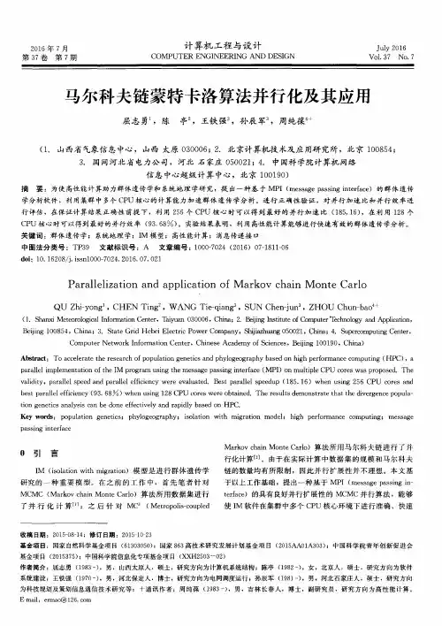

图2—1各种打包发送方式性能比较图2.1.3三种打包发送方式的适用环境通过以上测试结果,结合在实际并行环境中的问题需求,得出以下结论:(1)如果要发送的数据被存储在连续的数组单元中,我们只要使用第~种方法即可,即:使用MPI的通信函数的COUNT和DATATYPE两个参数,~次成批发送多个数据。
该方法没有任何附加通信开销,因为它既不用调用派生数据类型创建函数,也不用调用MPI—Pack/MPI—Unpack函数。
.(2)如果要发送的数据都含有相同的类型并且在内存中都是按规则的间隔存放(如:矩阵的一列元素),那么使用派生数据类型将比使用MPIPacIdMPl数据类型并且不规则地存储在内存空间中,则使用MPI—Type_indexed来创建派生数据类型将依然是更简单和更有效的方法。
最后,如果这些数据是不同类型的,并且我们需要重复地发送这些数据集(例如,行数,列数,等),最好也是使用派生数据类型,因为在整个通信中创建派生数据类型的开销只需要一次.而使用MPIPacIdMPIUnpack则每通信一次,就会有一次调用MPIPacI(,MPIUnpack的通信开销。
(3)剩下的一种情况就是;我们需要把一些不同类型的数据发送一次或者少数几次,这时,我们只需要把这些数据用MPI—Pack/MPI—Unpack打包发送,从而省去了创建MPl的派生数据类型的开销。
例如,在用MPICH来实现MPI的集群式高性能计算机上,在例子Getdata3中,需要12ms来创建派生数据类型,而在例子Getdata4中,它仅需要2ms去打包和拆包一个数据。
当然,由于数据的打包和拆包过程的不对称,时间的节约并不象它想象的那样明显。
也就是说:当进程0在打包数据时,其他进程都在闲置,整个函数将在打包和发送过◎上海大攀臻究生埝文ThePostgradumeThesisofShanghaiUniversity这一步并行的思想,可以用于所有类似问题的并行,所以,可以对此类并行闫联起銎l指导往的慝怒。

蒙特卡洛简介
蒙特卡洛(Monte Carlo)方法是一种统计技术,主要用于估算复杂系统的各种数值解。
其基本思想是通过随机抽样来模拟或估算一个过程,从而得到期望的统计结果。
以下是对蒙特卡洛方法的简要介绍:
历史背景:
蒙特卡洛方法得名于摩纳哥的蒙特卡洛赌场。
这个方法是在二战期间,由于需要解决核反应的随机扩散问题,由科学家们(如尤里·乌兰贝克、尼古拉·梅特罗波洛斯和约翰·冯·诺伊曼)在洛斯阿拉莫斯实验室中首次提出并使用的。
工作原理:
1. 随机抽样:根据某个分布(通常是均匀分布)生成大量随机样本。
2. 评估函数:对每个随机样本评估一个函数或模型。
3. 分析结果:基于评估的结果,计算所需的统计量(如均值、方差等)。
应用领域:
1. 金融:用于估算金融衍生品的价格和风险。
2. 物理:模拟复杂的物理过程,如核反应。
3. 工程:进行可靠性分析和风险评估。
4. 计算生物学:模拟生物分子的动力学。
5. 优化:搜索复杂的解空间以找到最优解。
优点:
1. 灵活性:可以应用于各种复杂的数学问题和模型。
2. 并行性:由于每个样本的评估是独立的,所以蒙特卡洛模拟非常适合并行计算。
缺点:
1. 收敛速度:需要大量的样本才能得到精确的估计。
2. 计算成本:可能需要大量的计算资源。
结论:
蒙特卡洛方法是一种强大而灵活的工具,它为解决许多复杂的数学和工程问题提供了手段。
尽管它有一些局限性,但在很多情况下,它都是最好的或唯一可行的解决方案。

第五章蒙特卡洛方法在机器学习和强化学习中,蒙特卡洛方法是一类基于随机抽样的方法,用于估计未知概率分布的特征或求解复杂的问题。
在本章中,我们将介绍蒙特卡洛方法的基本原理和应用领域。
1.蒙特卡洛方法的原理蒙特卡洛方法是通过利用随机抽样的规律来估计未知概率分布的特征。
其基本原理如下:(1)随机抽样:根据已知概率分布进行随机抽样,得到一系列样本。
(2)样本推断:利用得到的样本进行统计推断,从而估计未知概率分布的特征。
(3)结果评估:通过对估计结果进行评估,得到对未知概率分布的特征的估计值。
2.蒙特卡洛方法的应用领域蒙特卡洛方法广泛应用于估计数学问题、求解优化问题以及模拟高维空间中的复杂系统。
以下是一些蒙特卡洛方法的应用领域的示例:(1)数值计算:蒙特卡洛方法可以用于计算复杂的数学问题,如计算积分、求解微分方程等。
通过随机抽样和统计推断,可以得到对问题的近似解。
(2)优化问题:蒙特卡洛方法可以用于求解优化问题,如最大化或最小化函数的值。
通过随机抽样和统计推断,可以找到函数的全局最优解或局部最优解。
(3)统计推断:蒙特卡洛方法可以用于估计未知概率分布的特征,如均值、方差、分位数等。
通过随机抽样和统计推断,可以得到这些特征的近似值。
(4)模拟与优化:蒙特卡洛方法可以用于模拟高维空间中的复杂系统,如金融市场、交通网络等。
通过随机抽样和统计推断,可以对系统的行为进行建模和优化。
3.蒙特卡洛方法的算法步骤蒙特卡洛方法的算法步骤如下:(1)随机抽样:根据已知概率分布进行随机抽样,得到一系列样本。
(2)样本推断:利用得到的样本进行统计推断,从而估计未知概率分布的特征。
常见的推断方法有样本平均法、样本方差法等。
(3)结果评估:通过对估计结果进行评估,得到对未知概率分布的特征的估计值。
常见的评估方法有置信区间估计、假设检验等。
4.蒙特卡洛方法的优缺点蒙特卡洛方法具有以下优点:(1)简单易实现:随机抽样和统计推断是蒙特卡洛方法的基本步骤,易于理解和实现。
光子传输的蒙特卡罗方法在GPU 上的实现L´ aszl ´o Szirmay-Kalos 等翻译:吴涛这篇文章提出一个快速的蒙特卡罗方法来解决激光和gamma 射线光子在不均匀媒介中辐射传输方程问题。
激光传输在计算机图表算法中起着重大作用,比如高能gamma 射线就在医疗与物理中扮演重要角色。
实时图像的应用在速度上受到限制,因为我们通常想得到每秒至少20张图来获取运动的动态幻像。
快速模拟在人机交互系统中也十分重要,比如像放射疗法或者物理实验设计,这些地方用户可以放置一个源,并且希望得到辐射分配的迅速反馈。
多重散射模拟的速度在迭代断层摄像术重建方面也很重要,此时散射辐射要从实际的重建数据中,且要移除测量部分来估计,而重建仍然继续针对那些假设只代表不散射的部分剩余成分。
17.1光子传输的物理特性计算多重散射以及提出一种在不均匀媒介的实际方法更是困难重重。
最精确的逼近方法是依据蒙特卡罗方法的积分运算以及通过跟踪随机光子的物理模拟现象,来计算他们的总贡献。
光子与媒介粒子在该点碰撞的条件概率密度由消光系数(,)t x σν 定义,如果粒子密度不均匀,它则由光子频率ν以及位置x 来确定。
消光系数通常可以用材料密度()C x 和一个仅与频率有关的因子的乘积来表达。
光子在碰撞之外还会被反射与吸收。
反射的概率称为反照率,用()a ν表示。
随机反射方向用两个球坐标轴描述:散射角θ和方位角ϕ(图17.1)。
源点与新的方向的散射角θ的概率密度可能与频率有关故用物理模型来描述(我们用瑞利散射【12】模型来模拟激光光子,用Klein-Nishina 公式【11】【13】来计算gamma 光子)。
方位角ϕ的概率密度鉴于轴向对称分布故而是均衡的。
图17.1光子在媒介中的散射。
能量为0E 的入射光子与材料的粒子碰撞。
因为碰撞,光子的方向和能量将改变。
新的方向由散射角θ和方位角ϕ指定。
新的光子能量E 由入射光子能量和散射角确定。
基于gpu并行计算的蒙特卡洛方法计算圆周率1. 引言1.1 概述蒙特卡洛方法是一种通过随机模拟的方式解决问题的数学计算方法。
在很多科学领域中,特别是需要进行复杂的数值计算和模拟的问题中,蒙特卡洛方法被广泛应用。
它通过使用随机样本来近似求解问题,具有较高的精确性和灵活性。
本篇文章主要探讨了基于GPU并行计算的蒙特卡洛方法用于计算圆周率的应用。
GPU并行计算具有强大的计算能力和高效的数据处理能力,因此可以大大提高蒙特卡洛方法的计算效率。
1.2 文章结构本文包含以下几个部分:引言、GPU并行计算简介、蒙特卡洛方法简介、基于GPU的蒙特卡洛方法计算圆周率以及结论和展望。
首先,引言部分将介绍本文所要讨论的主题,并对文章的结构进行简单描述。
其次,在"2. GPU并行计算简介"部分将对GPU并行计算进行详细阐述,包括其基本原理、并行计算优势以及在科学计算中的应用。
然后,在"3. 蒙特卡洛方法简介"部分将对蒙特卡洛方法的原理进行概述,并介绍其在不同领域的应用。
同时,还将与传统计算方法进行对比,以突出蒙特卡洛方法的优势和适用性。
接下来,在"4. 基于GPU的蒙特卡洛方法计算圆周率"部分将重点讨论基于GPU 并行计算实现的蒙特卡洛方法用于计算圆周率的具体步骤。
这一部分将解释圆周率相关概念、Monte Carlo模拟过程分析,并详细描述使用GPU并行计算实现这一过程所需的步骤和技术。
最后,在"5. 结论和展望"部分总结全文并发现主要内容。
我们还将讨论可能的改进方向以及未来发展趋势,旨在启发读者进一步研究和探索基于GPU并行计算的蒙特卡洛方法。
1.3 目的本文旨在介绍利用GPU并行计算加速蒙特卡洛方法计算圆周率的原理和实践,探讨其在提高效率和精度方面的优势。
通过本文,读者将了解到GPU并行计算在科学计算中的重要作用,并对蒙特卡洛方法的原理和应用有更深入的理解。
蒙洛卡特算法蒙洛卡特算法是一种基于随机抽样技术的数值计算方法,广泛应用于风险评估、金融衍生品定价、物理模拟等众多领域。
本文将对蒙洛卡特算法的原理、应用以及优势进行介绍。
一、蒙洛卡特算法原理蒙特卡洛算法是一种随机化算法,基于随机抽样的方法获取样本来求解问题。
直接蒙特卡洛算法是一种非常原始的方法,将问题转化为一个期望值,使用随机抽样的方法进行估计。
而蒙洛卡特算法则是通过改进直接蒙特卡洛算法,使得随机抽样的效率更高。
具体来说,蒙洛卡特算法首先通过随机抽样的方法生成多个独立的随机数序列,这些序列称为样本。
然后,将这些样本输入到函数中进行计算,最后对计算结果进行统计分析得到估计值。
蒙洛卡特算法有以下几个特点:1. 独立性。
样本之间应该是相互独立的,这意味着每个样本都是完全独立于其他样本的,并且可以多次使用。
2. 随机性。
随机抽样的过程应该是完全随机的,这意味着每个样本的值应该是随机的,并且应该具有相同的概率分布。
3. 代表性。
样本应该是代表性的,这意味着样本的数量应该足够大,以及样本应该来自于整个概率分布的区域。
4. 收敛性。
当样本数量足够大时,蒙洛卡特算法会收敛于真值。
二、蒙洛卡特算法应用1. 风险评估。
用蒙洛卡特算法进行风险评估,可以帮助投资者更加准确地评估投资的风险。
2. 金融衍生产品定价。
蒙洛卡特算法可以帮助金融衍生产品的定价,例如期权、期货等。
3. 物理模拟。
使用蒙洛卡特算法可以模拟物理系统,例如量子场论、蒙特卡洛模拟等。
4. 优化模型。
蒙洛卡特算法可以用于优化模型,例如寻找一个函数的最小值或最大值。
三、蒙洛卡特算法优势1. 可分布计算。
蒙洛卡特算法允许在分布式计算环境下运行,这使得它能够利用并行计算的优势来提高计算效率。
2. 适应高维数据。
相比于其他的数值计算方法,蒙洛卡特算法在处理高维数据时表现更加优秀。
3. 不要求导数。
相比较于一些需要求导数的数值计算方法,例如最优化算法和差分方程算法,蒙洛卡特算法不需要对函数进行求导。
并行蒙特卡罗方法的应用作者:申杰王文凡来源:《电脑知识与技术(学术交流)》2009年第22期摘要:本文采用蒙特卡罗方法对欧式期权定价问题进行模拟,并用可移植消息传递标准MPI 在分布式存储结构的机群系统上设计并实现了并行算法。
该算法有效的解决了金融计算中巨大计算量的问题,在很大程度上提高了计算效率,缩短了计算时间,获得了很好的性能。
关键词:蒙特卡罗方法;欧式期权定价;消息传递;并行计算中图分类号:TP301.6文献标识码:A文章编号:1009-3044(2009)22-0000-00现代科技中出现许多复杂的随机性问题,用确定性方法给出其近似解是很困难的,甚至是不可能的。
用蒙特卡罗方法进行模拟是解决这类随机性问题的一个有效途径。
蒙特卡罗方法是金融分析最为常用的方法,有时甚至是唯一的方法[1,2]。
然而蒙特卡罗方法一次有效的模拟过程通常需要上百万次的实验,计算量相当大,用串行算法需要耗费大量的人力物力。
为了解决此类问题,可采用高性能并行计算方法。
并行计算方法是用并行计算机获得更快的计算速度,减少解决问题所需时间[3]的一种方法。
特别是对新出现的具有巨大挑战性的计算量超大的问题,不使用并行计算方法是根本无法解决的。
而且并行计算方法可以节省投入,以较低的成本完成串行计算需要大量时间来完成的计算任务。
1 蒙特卡罗方法的基本原理蒙特卡罗(Monte Carlo)方法是与一般数值计算方法有很大区别的一种特殊计算方法。
它以概率统计理论为基础,通过在随机变量的概率分布中随机选取数字,产生一种符合该随机变量概率分布特性的随机数序列,作为输入序列进行模拟实验,并求解[4]。
在抽取大量特定的不均匀概率分布的随机数序列时,可行的方法是先产生一种均匀分布的伪随机数序列,然后转换成特定概率分布要求的伪随机数序列,以此作为模拟实验的输入变量序列,再进行模拟,最后进行统计计算,求出所求参数的近似值。
本文以欧式期权定价为研究对象,采用蒙特卡罗方法对其定价的基本步骤如下:1)建立概率模型。
蒙特卡罗方法计算VAR的并行实现
周阳
【期刊名称】《信息与电脑》
【年(卷),期】2017(000)005
【摘要】当今经济全球化、金融全球化进程加快,市场竞争愈演愈烈.建立一个良好的风险管理系统已成为各金融单位面临的重要问题.在众多的风险管理方法中最具代表性的是Value at Risk(VAR)方法.而计算VAR常见的三种方法中,Monte Carlo模拟最为有效.由于蒙特卡罗模拟需要大量数据,所以并行计算在计算VAR中非常重要.笔者基于Monte Carlo方法计算VAR的原理构造C++算法,并用基于API、OpenMP、MPI三种多核并行算法,比较分析出了适合科学计算研究的并行算法.
【总页数】4页(P109-112)
【作者】周阳
【作者单位】中国石油大学(华东) 理学院,山东青岛 266580
【正文语种】中文
【中图分类】TL329.2
【相关文献】
1.合成孔径雷达并行成像算法研究及在曙光3000并行计算机上的实现 [J], 龙卉;皮亦鸣;黄顺吉
2.蒙特卡罗方法模拟计算圆周率--基于R语言的实现方法 [J], 彭滔;魏雷阳
3.基于多态并行处理器的生物计算并行实现 [J], 刘玉荣;李涛
4.利用蒙特卡罗方法与拟蒙特卡罗方法计算定积分 [J], 韩俊林;任薇
5.并行计算平台的模拟与并行算法的实现 [J], 熊仕勇
因版权原因,仅展示原文概要,查看原文内容请购买。
并行fortran蒙特卡罗编程
并行Fortran蒙特卡罗编程是使用Fortran编程语言在并行计算环境下实现蒙特卡罗方法的编程方法。
蒙特卡罗方法是一种通过随机采样和统计分析来求解数学问题的方法,广泛应用于模拟、优化、风险分析等领域。
蒙特卡罗方法的运行时间通常比较长,因此它常常需要借助并行计算的能力来加速计算过程。
在并行Fortran蒙特卡罗编程中,可以使用一些并行编程的特性和库来实现并行计算。
比如,可以使用Fortran的共享内存并行机制(OpenMP)来将计算任务分配给多个线程并发执行,而每个线程独立地进行随机采样和统计分析。
此外,还可以使用一些并行数值计算库如MPI(Message Passing Interface)来实现分布式内存并行计算,使得多个计算节点能够协同工作,加速计算过程。
并行Fortran蒙特卡罗编程的主要挑战是如何将计算任务有效地划分成多个子任务,并合理地管理和调度这些子任务的执行。
同时还需要注意保证随机数的独立性和一致性,以确保模拟结果的准确性。
总的来说,并行Fortran蒙特卡罗编程可以有效地利用多核处理器和分布式计算资源,加速蒙特卡罗模拟的计算过程,提高计算效率和吞吐量。
Monte Carlo Methods in Parallel ComputingChuanyi Ding ding@Eric Haskin haskin@Copyright by UNM/ARCNovember 1995OutlineWhat Is Monte Carlo?Example 1 - Monte Carlo Integration To Estimate PiExample 2 - Monte Carlo solutions of Poisson's EquationExample 3 - Monte Carlo Estimates of ThermodynamicPropertiesGeneral Remarks on Parallel Monte CarloWhat is Monte Carlo?• A powerful method that can be applied to otherwise intractable problems• A game of chance devised so that the outcome from a large number of plays is the value of the quantity sought•On computers random number generators let us play the game•The game of chance can be a direct analog of the process being studied or artificial•Different games can often be devised to solve the same problem •The art of Monte Carlo is in devising a suitably efficient game.Different Monte Carlo ApplicationsRadiation transportOperations researchNuclear criticalityDesign of nuclear reactorsDesign of nuclear weaponsStatistical physicsPhase transitionsWetting and growth of thin films Atomic wave functions and eigenvalues Intranuclear cascade reactions Thermodynamic propertiesLong chain coiling polymersReaction kineticsPartial differential equationsLarge sets of linear equations Numerical integrationUncertainty analysisDevelopment of statistical testsCell population studiesCombinatorial problemsSearch and optimizationSignal detectionWarGamesProbability Theory•Probability Density Function•Expection Value (Mean)•Variance and Standard DeviationSampling a Cumulative Distribution FunctionFundamental Theorem•Sample Mean, a Monte Carlo estimator of the expection value•Fundamental theorem of Monte CarloStatistical Error in MC Estimator•Variance and Standard Deviation of Estimator•Central Limit TheoremExample 1 - Monte Carlo Integration to Estimate Pi • A simple example to illustrate Monte Carlo principals•Accelerate convergence using variance reduction techniques o Use if expectation valueso Importance sampling•Adapt to a parallel environmentMonte Carlo Estimate of PiWhen to Consider Monte Carlo Integration•Time required for Monte Carlo Integration to a standard error epsilon•Time required for numerical integration in n dimensions with trunction error of order h to the power k. (Note: k for Simpson's 1/3 rule is 4)•Rule of ThumbSerial Monte Carlo Algoritm for PiRead NSet SumG = 0.0Do While i < NPick two random numbers xi and yiIf (xi*xi + yi*yi £ 1) thenSumG = SumG + 1EndifEnddoGbar = SumG / NSigGbar = Sqrt(Gbar - Gbar2)Print N, Gbar, SigGbarParallelization of Monte Carlo Integration•If message passing time is negligibleo For same run time, error decreases by factor of Sqrt(p)o For same accuracy, run time improves by a factor of p •Should use same random number generator on each node (easy for homogeneous architecture)Monte Carlo Estimates of PiNumber of Batch CPU Standard True Processors Size Time(sec) Deviation Error--------------------------------------------------------1 100,000 0.625 0.0050.00182 50,000 0.25 0.0050.00374 25,000 0.81 0.0050.0061--------------------------------------------------------•To try this problem, run MCPI by :% cd% cp -r /usr/local/mc .% cd mc/mcpi% run•Parallel MC Estimate of Pi, mcpi.C1. Creating the random number generatorsfor ( int i=0; i < num_dimension; i++) { // create r.n. generator// the seeds are different for the processorsseed = (myRank + 1) * 100 + i * 10 + 1;if ( seed == 0 )rand[i] = new RandomStream(RANDOMIZE);elserand[i] = new RandomStream( seed );}2. Each processors will run num_random / numProcs random walksfor ( i=myRank; i < num_random; i+=numProcs ) { // N random walks2a. Generating random numbersfor ( int i1=0; i1 < num_dimension; i1++) {ran[i1] = rand[i1]- > next();}2b. Calculating for integrationif ( inBoundary( ran, num_dimension ) ) {myPi += f( ran, num_dimension ) * pdf( ran, num_dimension ); count++;}}3. Calculating Pi from each processormyPi = 4 * myPi / num_random;MPI_Reduce(&myPi, &pi, 1, MPI_DOUBLE, MPI_SUM, 0,MPI_COMM_WORLD);4. Output the results and standard deviation, sigmaif (myRank == 0) {cout << "pi is = " << pi<< " sigma = " << 4 * sqrt( (pi/4 - (pi/4)*(pi/4)) / num_random)<< " Error = " << abs(pi - PI25DT) << endl;}Variance Reduction by Use of Expectation Values •For original sampling•Carry out integrations from 0 to 1/Sqrt(2) analytically •Sample from 1/Sqrt(2) to 1•Variance = 0.0368•Speedup by (0.168/0.0368) > 4.5 for same accuracy.•Carry out integration over one coordinate analytically.Variance Reduction by Important Sampling•Say•Can use a different pdf•Greatest reduction in variance whenA Product h(x)f(x) and a possible f~(x)Using Qualitative Information•Smaller values of x contribute more to integral•Indicated change in pdf reduces varianceo from 0.0498o to 0.00988•Speedup > 5Omniscience Yields Zero Variance•Choose lambda by requiring integral to be oneletthen•For h(x) = Sqrt(1-x**2), the variance is reduced to zero.•Boils down to finding a simple function that approximates that to be integrated.Example 2 - Solving a Partial Differential Equation by Monte Carlo •Poisson's equation•Geometry•Source:•Boundary condition: u(x,y) = 0 on boundaryPoisson's Equation As a Fixed Random Walk Model•Using a finite difference approximation,•SolvingFixed Random Walk Solution Algorithm•From point (i,j), start a random walk. Probability of moving to each of the adjacent nodes is 1/4.•Generate a random number to determine which way to move•Add g(x,y) at the new position•Repeat this until a boundary is reached•After N random walks, the estimate of u at (i,j) isParallel Strategies for Fixed Random Walk•When solving at all grid pointso Start from boundaryOutside to insideRow by rowBoundary updating depends on relative message passingtimeUpdate only within each processor (poisson4.C)Update globally when any processor finishes a point(poisson5.C)May help to decompose problem (poisson.C) •When solving at only a few point(s) may want to split walks for point between processorsResults for Fixed Random Walk in Solid SlabNumber of Walks/ CPU StandardProcessors Point Time u(20,20) Deviation-----------------------------------------------------1 1000 400 0.0483 0.000162a 1000 270 0.0480 0.000204a 1000 165 0.0485 0.00020=====================================================2b 1000 313 0.0477 0.000204b 1000 234 0.0480 0.00029----------------------------------------------------a - Update all processors at same timeb - Only update whthin individual processor•To apply Monte Carlo to a 1x1 slab with a 0.5x0.5 center hole, run poisson4.C and poisson5.C by :% cd% cd mc/poisson4% run•The Structure of poisson.C1. // Set boundary conditionboundary(nx, ny);2. Devide the initial region into 4 sub-region if necessary2.a Evaluate the virtual parallel inner boundary line2.b Evaluate the virtual vertical inner boundary line2.c Initialize boundary for each sub-region3. // Calcalute u for (ix,iy) of each regionwhile ( 1 ) {3.a // Calculate u[ix][iy] for a point (ix,iy), and send it to otherssendU( rand, ix, iy, delta );3.b // Receives u[iix][iiy] from the other processorsfor ( int i = 0; i < numProcs; i++) {if (i != myRank) {MPI_Recv(&uRec, 1, MPI_DOUBLE, i, 99,MPI_COMM_WORLD,&status);if (uRec <= -1000) flag = 1;else {ixp = ix + (i - myRank); // the index of inner boundary,iyp = iy; // u at this cell received from// another processor if ( ixp > (nx2[iRegion] - 1) ) {ixp = nx1[iRegion] + (ixp - nx2[iRegion]) + 1; iyp = iy + 1;}3.c // Set this point as a boundaryu[ixp][iyp] = uRec;onBoundary[ixp][iyp] = 1;}}3.d // Set ix, iy of next node for the processorix += numProcs;if ( ix > (nx2[iRegion] - 1) ) {ix = nx1[iRegion] + (ix - nx2[iRegion]) + 1;iy++;}assert( ((ix < nx) && (iy < ny)), " out of given domain");}Floating Random Walk Solution Algorithm (point.C) •The potential at the center of a circle of radius r, which liesentirely within the region is•Start a walk at point (i,j).•Construct a circle centered at point (i,j) with radius equal to the shortest distance to a boundary.•Select an angle from the x-direction randomly between 0 and 2 Pi.•Follow this direction to a new location on the circle•When the new position is within epsilon of a boundary add the boundary potential and begin a new walk.Sample Results for Floating Random Walk in Solid SlabNumber of CPU Time CPU TimeProcessors 1000 Walks 100,000 walks------------------------------------------1 0.44 3.062 0.5 2.54 0.5 1.4------------------------------------------•To try the floating random walk method, run the code point.C by :% cd% cd mc/point% run•The structure of point.C1. // Set boundary condition2. // Set the points which are evaluated.for (int i=0; i < numPoint; i++) {x[i] = (i + 1.) / ( numPoint + 1. );y[i] = (i + 1.) / ( numPoint + 1. );}3. Evaluate each pointfor ( i=0; i < numPoint; i++ ) {... ...3.a All processors run for one same pointfor ( int ir=myRank; ir < num_random; ir+=numProcs ) {// initilaizing the position of the point for each random walkxx = x[i];yy = y[i];while (1) {// calculating the minimum distance of selected point// to the boundaryminDist = MinDist(xx, yy, side);if ( minDist < acceptDist ) break;// each processor generates a random number, and make a random// move, the point moves randomly to any point at the circle// with a radius of minDist, and centered at (xx, yy) double ran = rand->next();xx += minDist * sin(2*pi*ran);yy += minDist * cos(2*pi*ran);}// sumtempU = EvalPoint( xx, yy, side );myU += tempU;mysqU += tempU * tempU;} // end of a ramdom walkmyU /= num_random;mysqU /= num_random;3.b // Sum the results from all processorsMPI_Reduce(&myU, &u, 1, MPI_DOUBLE, MPI_SUM, 0, MPI_COMM_WORLD);MPI_Reduce(&mysqU, &sqU, 1, MPI_DOUBLE, MPI_SUM, 0,MPI_COMM_WORLD);3.c // print outif ( myRank == 0 )cout << "At the point of " << x[0] << ", " << y[0] << " , u is = " << u<< " , sigma = " << sqrt( (sqU - u*u) / num_random);Example 3 - Monte Carlo Estimate of Thermodynamic Properties •Consider a system of atoms with a finite number of configurations.•Let En denote energy of the n-th configuration•The probability that the system is in the n-th configuration is•The expectation value of observable property A isWhy not determine such expectation values exactly?•Consider a 10x10x10 cubic crystal of atoms in which each atom has only two possible states.Number of Possible Configurations = 2**1000 •Summing at a rate of one million configurations per second, Time Required for Exact Calculation = 10**288 years •In contrast, to achieve 1% accuracy, using the Monte Carlo method, about 10,000 terms must be summed.Metropolis Algorithm•Follows a sequence of configurations•Pn(C) is probability of the n-th observation in configuration C •T(C->C') is probability of making a transition from state C to state C'•Probability of remaining in state C is•Master equation for this Markov process is•Rearranging master equation•In steady state, transition probability must be independent of time and must goto zero; that is Pn(C) must be the steady state function P(C) and P(C)T(C->C') = P(C')T(C'->C) •Since P(C) is proportional to Exp(-Ec/kT), this means•What transition probability will give the correct probability function P(C)?•The answer is not unique•All we need is a function T(C->C') that satisfies the detailed balance P(C)T(C->C') = P(C')T(C'->C)•One transition function that is often used is:Example 3 - 2D Ising Model•Simplify to a square lattice of N=LxL atoms. Each atom has only a spin degree of freedom,spin = +1 (up),spin = -1 (down)•The energy of the n-th given configuration is•For a given temperature T, the specific heat C and magnetic x susceptability per site can be estimated as2D Ising Metropolis Algorithm•Let n = 0, and start with an arbitrary configuration, for example, all spins up.•Pick two random integers x and y between 1 and L. Let DelE be the change in energy caused by changing the value of the spin at (x,y).•Increase n by 1. If DelE < 0, accept the change. If DelE > 0 accept the new configuration with probability Exp(-DelE/kT). Go to step2.2D Ising - Metropolis Algorithm (Cont.)•The Metropolis algorithm produces a series of configurations that eventually approaches a sampling sequence for the discreteprobability function•It is difficult to predict how long it will take for the Metropolis algorithm to reach this asymptotic state.•This is usually determined empirically by seeing whether the average over a large number of configurations converges.•Note: The algorithm requires DelE not E be calculated for each trial change. DelE is generally much easier to calculate.Example 3 - Monte Carlo Estimates of Thermodynamic Properties •Estimate heat capacity and magnetic susceptibility as functions oftemperature.•Have each processor handle a separate temperature calculation.•INSERT PARALLEL FLOW FIGURE HEREResults for 2D Ising Problem•INSERT RESULTS FIGURE HERE•To run this problem, use the code ising.C by :% cd% cd mc/ising% run•The structure of ising.C1. // Set the parameters and initializeinitialize( l, h, v );2. // Each processor evaluates the properties of system at atemperaturefor (int i=myRank; i < num_runs; i += numProcs) {double tau = tauMin + i * delTau;2.a // Make the atoms of system random distributedfor (int j=0; j < 100*l*l; j++ ) {ran1 = rand1->next();ran2 = rand2->next();makeMove( l, h, v, ran1, ran2, tau );}2.b // Go to random walks, and add the energy of each statefor ( int i1=0; i1 < num_random; i1++ ) {ran1 = rand1->next();ran2 = rand2->next();makeMove( l, h, v, ran1, ran2, tau );sumM += abs(m);sumM2 += m * m;sumE += e;sumE2 += e * e;}2.c Calculate the thermal propertiesdouble aveM = sumM / num_random;double aveM2 = sumM2 / num_random;double aveE = sumE / num_random;double aveE2 = sumE2 / num_random;double delSqM = aveM2 - aveM * aveM;double delSqE = aveE2 - aveE * aveE;aveM /= l * l;aveE /= l * l;double temp = tau * tau * l * l;double chi = delSqM / temp;double specHeat = delSqE / temp;General Observations Regarding Paralle Monte Carlo •Applicability of Parallel Monte Carloo Most serial Monte Carlo codes are readily adaptable to a parallel environmento Strengths are still forMulti-dimensional problemsComplex geometrieso Variance reduction techniques must still be tailored to the specific problem (possible exception - stratified samplingfor numerical integration) inherently serial must bemodified for effective parallelizationo Care must be taken to assure reproducible results •Pseudorandom Number Generation on Parallel Computerso Fast RNGs with long periods requiredCongruentialxnew = (a xold + c) mod m,fast, typically repeats after a few billionnumbersMarsagliaFaster, a million numbers per second on a laptopperiod of 2**1492 for 32 bit numbers o Reproducibility highly desirableo Must assure calculations on different processors are independentLehmer Tree•Amdahl's Lawo T1 = task execution time for a single processoro Tm = execution time for the multiprocessing portiono To = execution time of the sequential and communications portion (overhead)Speedup = T1/(Tm+To)o For many Monte Carlo applications Tm is approximately T1/P where P is the number of processorsEfficiency = Speedup/P = 1/(1+F)o F = P*To/T1 is the overhead factor.•Efficiency versus Number of Processors•Overhead Timeo Initialization timeo Message passing timeTends to increase nonlinearly with PTends to increase with size of problem (information passed)o Sleep timeProcessor to processor variations resulting fromrandomnessCan't aggregate results until all processors doneLoad balancing required in heterogeneous systems。