第11章 收益和风险:资本资产定价模型
- 格式:ppt
- 大小:2.20 MB
- 文档页数:62
资本资产定价模型
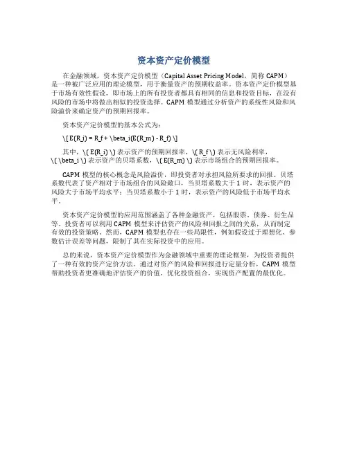
在金融领域,资本资产定价模型(Capital Asset Pricing Model,简称CAPM)是一种被广泛应用的理论模型,用于衡量资产的预期收益率。
资本资产定价模型基于市场有效性假设,即市场上的所有投资者都具有相同的信息和投资目标,在没有风险的市场中将做出相似的投资选择。
CAPM模型通过分析资产的系统性风险和风险溢价来确定资产的预期回报率。
资本资产定价模型的基本公式为:
\[ E(R_i) = R_f + \beta_i(E(R_m) - R_f) \]
其中,\( E(R_i) \) 表示资产的预期回报率,\( R_f \) 表示无风险利率,
\( \beta_i \) 表示资产的贝塔系数,\( E(R_m) \) 表示市场组合的预期回报率。
CAPM模型的核心概念是风险溢价,即投资者对承担风险所要求的回报。
贝塔系数代表了资产相对于市场组合的风险敞口,当贝塔系数大于1时,表示资产的风险大于市场平均水平;当贝塔系数小于1时,表示资产的风险低于市场平均水平。
资本资产定价模型的应用范围涵盖了各种金融资产,包括股票、债券、衍生品等。
投资者可以利用CAPM模型来评估资产的风险和回报之间的关系,从而制定有效的投资策略。
然而,CAPM模型也存在一些局限性,例如假设过于理想化、参数估计误差等问题,限制了其在实际投资中的应用。
总的来说,资本资产定价模型作为金融领域中重要的理论框架,为投资者提供了一种有效的资产定价方法。
通过对资产的风险和回报进行定量分析,CAPM模型帮助投资者更准确地评估资产的价值,优化投资组合,实现资产配置的最优化。

第11章 资本资产定价模型 选择:1、零贝塔证券的预期收益率是什么?(d ) a. 市场收益率 b. 零收益率 c. 负收益率 d. 无风险收益率2、CAPM 模型认为资产组合收益可以由( c )得到最好的解释。
a. 经济因素 b. 特有风险 c. 系统风险 d. 分散化3、根据C A P M 模型,贝塔值为1 . 0,阿尔法值为0的资产组合的预期收益率为(d ): a. 在M r 和F r 之间 b. 无风险利率F r c. (M r -F r ) d. 市场预期收益率M r简答:1、市场上存在着许多类型的基金,如增长型基金和稳健型基金等。
这与分离定理矛盾吗?为什么?2、以下说法是对还是错?a. Beta 值为零的股票的预期收益率为零。
b. CAPM 模型表明如果要投资者持有高风险的证券,相应地也要求更高的回报率。
c. 通过将0 . 7 5的投资预算投入到国库券,其余投入到市场资产组合,可以构建Beta 值为0 . 7 5的资产组合。
计算 1、已知股票A 、B 收益率的标准差分别为0.25和0.3,与市场的相关系数分别为0.5和0.3,市场期望收益率与标准差分别为0.12和0.1,无风险利率为0.05。
(1)计算A 、B 及A 、B 的等权数组合的Beta 值;(2)利用CAPM ,计算A 、B 及A 、B 的等权数组合的期望收益率。
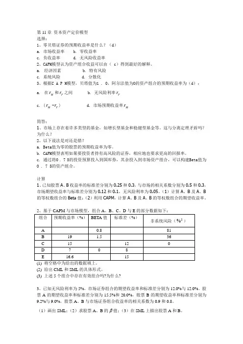
(2) 给出CML 和SML 的具体形式。
(3) 上述5个组合中存在有效组合吗?为什么?3、已知无风险利率为5%,市场证券组合的期望收益率和标准差分别为12.0%与12.0%。
股票A 的期望收益率和标准差分别为15.5%和20.0%,股票B 的期望收益率和标准差分别为9.2%与9.0%,股票A 、B 与市场证券组合收益率的相关系数为0.9和0.8。
(1)画出SML ;(2)求股票A 、B 的 值;(3)在SML 上描出股票A 和B 。
第十一章资本资产定价模型在金融领域,资本资产定价模型(Capital Asset Pricing Model,简称 CAPM)是一个具有重要地位的理论模型。
它为投资者理解资产的预期收益与风险之间的关系提供了关键的框架。
首先,我们来了解一下什么是资本资产定价模型。
简单来说,CAPM 试图解释在均衡市场中,资产的预期收益率是如何由其系统性风险所决定的。
这里的系统性风险,通常用贝塔(β)系数来衡量。
贝塔系数反映了一项资产相对于整个市场的波动程度。
如果一项资产的贝塔系数大于 1,意味着它的波动幅度比市场平均水平大,属于高风险高收益的资产;反之,如果贝塔系数小于 1,则其波动相对较小,风险也较低。
而当贝塔系数等于 1 时,该资产的风险和收益与市场平均水平相当。
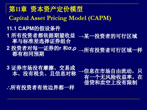
那么,资本资产定价模型是如何得出的呢?它基于一系列的假设条件。
比如说,投资者是理性的,他们追求风险调整后的最大收益;市场是完美的,不存在交易成本、税收等因素的干扰;信息是完全对称的,所有投资者都能同时获得相同的信息。
在实际应用中,资本资产定价模型具有多方面的用途。
对于投资者而言,它可以帮助评估不同资产的预期收益,从而做出更明智的投资决策。
比如,通过计算资产的贝塔系数,结合无风险利率和市场预期收益率,投资者能够大致估计该资产的合理预期回报。
如果实际预期收益高于模型计算出的结果,那么可能意味着这是一个值得投资的机会;反之,如果低于计算结果,则可能需要重新考虑投资策略。
对于企业来说,CAPM 也有重要意义。
在进行项目评估和资本预算时,企业可以利用该模型确定项目所需的最低回报率,从而判断项目是否具有经济可行性。
此外,它还可以帮助企业确定合理的资本成本,为融资决策提供依据。
然而,资本资产定价模型也并非完美无缺。
它的假设条件在现实中往往难以完全满足。
例如,投资者并不总是完全理性的,市场也并非完全有效,信息不对称的情况时有发生。
而且,贝塔系数的计算可能会受到市场波动和数据选取的影响,从而导致结果的不确定性。

第十一章:收益和风险:资本资产定价模型1.系统性风险通常是不可分散的,而非系统性风险是可分散的。
但是,系统风险是可以控制的,这需要很大的降低投资者的期望收益。
2.(1)系统性风险(2)非系统性风险(3)都有,但大多数是系统性风险(4)非系统性风险(5)非系统性风险(6)系统性风险3.否,应在两者之间4.错误,单个资产的方差是对总风险的衡量。
5.是的,组合标准差会比组合中各种资产的标准差小,但是投资组合的贝塔系数不会小于最小的贝塔值。
6. 可能为0,因为当贝塔值为0 时,贝塔值为0 的风险资产收益=无风险资产的收益,也可能存在负的贝塔值,此时风险资产收益小于无风险资产收益。
7.因为协方差可以衡量一种证券与组合中其他证券方差之间的关系。
8. 如果我们假设,在过去3 年市场并没有停留不变,那么南方公司的股价价格缺乏变化表明该股票要么有一个标准差或贝塔值非常接近零。
德州仪器的股票价格变动大并不意味着该公司的贝塔值高,只能说德州仪器总风险很高。
9. 石油股票价格的大幅度波动并不表明这些股票是一个很差的投资。
如果购买的石油股票是作为一个充分多元化的产品组合的一部分,它仅仅对整个投资组合做出了贡献。
这种贡献是系统风险或β来衡量的。
所以,是不恰当的。
10. The statement is false. If a security has a negative beta, investors would want to hold the asset to reduce the variability of their portfolios. Those assets will have expected returns that are lower than the risk-free rate. To see this, examine the Capital Asset Pricing Model:E(R S) = R f + S[E(R M) – R f] If S < 0, then the E(R S) < R f11. Total value = 95($53) + 120($29) = $8,515The portfolio weight for each stock is:WeightA = 95($53)/$8,515 = .5913 WeightB = 120($29)/$8,515 = .4087 12.Total value = $1,900 + 2,300 = $4,200So, the expected return of this portfolio is:E(R p) = ($1,900/$4,200)(0.10) + ($2,300/$4,200)(0.15) = .1274 or 12.74%13. E(R p) = .40(.11) + .35(.17) + .25(.14) = .1385 or 13.85%14. Here we are given the expected return of the portfolio and the expected return of each asset in the portfolio and are asked to find the weight of each asset. We can use the equation for the expected return of a portfolio to solve this problem. Since the total weight of a portfolio must equal 1 (100%), the weight of Stock Y must be one minus the weight of Stock X. Mathematically speaking, this means:E(R p) = .129 = .16w X + .10(1 –w X)We can now solve this equation for the weight of Stock X as:.129 = .16w X + .10 – .10w X w X = 0.4833So, the dollar amount invested in Stock X is the weight of Stock X times the total portfolio value, or: Investment in X = 0.4833($10,000) = $4,833.33And the dollar amount invested in Stock Y is:Investment in Y = (1 – 0.4833)($10,000) = $5,166.6715. E(R) = .2(–.09) + .5(.11) + .3(.23) = .1060 or 10.60%16. E(RA) = .15(.06) + .65(.07) + .20(.11) = .0765 or 7.65%E(RB) = .15(–.2) + .65(.13) + .20(.33) = .1205 or 12.05%17. E(R A) = .10(–.045) + .25 (.044) + .45(.12) + .20(.207) = .1019 or 10.19%方差=.10(–.045 – .1019)⌒2 + .25(.044 – .1019)⌒2 + .45(.12 – .1019)⌒2 + .20(.207 – .1019)⌒2 = .00535标准差= (.00535)1/2 = .0732 or 7.32%18. E(R p) = .15(.08) + .65(.15) + .20(.24) = .1575 or 15.75%If we own this portfolio, we would expect to get a return of 15.75 percent.19. a.Boom: E(R p) = (.07 + .15 + .33)/3 = .1833 or 18.33%Bust: E(R p) = (.13 + .03 .06)/3 = .0333 or 3.33%E(Rp) = .80(.1833) + .20(.0333) = .1533 or 15.33%b. Boom: E(R p)=.20(.07) +.20(.15) + .60(.33) =.2420 or 24.20%Bust: E(R p) =.20(.13) +.20(.03) + .60( .06) = –.0040 or –0.40%E(R p) = .80(.2420) + .20( .004) = .1928 or 19.28%P的方差= .80(.2420 – .1928)⌒2 + .20( .0040 – .1928)⌒2 = .0096820.a.Boom: E(R p) = .30(.3) + .40(.45) + .30(.33) = .3690 or 36.90%Good: E(R p) = .30(.12) + .40(.10) + .30(.15) = .1210 or 12.10%Poor: E(R p) = .30(.01) + .40(–.15) + .30(–.05) = –.0720 or –7.20%Bust: E(R p) = .30(–.06) + .40(–.30) + .30(–.09) = –.1650 or –16.50%E(R p) = .20(.3690) + .35(.1210) + .30(–.0720) + .15(–.1650) = .0698 or 6.98%b. p⌒2 = .20(.3690 – .0698)⌒2 + .35(.1210 – .0698)⌒2 + .30(–.0720 – .0698)⌒2 + .15(–.1650 – .0698)⌒2 = .03312p的标准差= (.03312)⌒1/2 = .1820 or 18.20%21. β= .25(.75) + .20(1.90) + .15(1.38) + .40(1.16) = 1.2422.βp = 1.0 = 1/3(0) + 1/3(1.85) + 1/3(βX) βX = 1.1523.E(R i) = R f + [E(R M) – R f] ×βiE(R i) = .05 + (.12 – .05)(1.25) = .1375 or 13.75%24. We are given the values for the CAPM except for the of the stock. We need to substitute these values into the CAPM, and solve for the of the stock. One important thing we need to realize is that we are given the market risk premium. The market risk premium is the expected return of the market minus the risk-free rate. We must be careful not to use this value as the expected return of the market. Using the CAPM, we find:E(R i) = .142 = .04 + .07βi 则βi = 1.4625. E(R i) = .105 = .055 + [E(R M) – .055](.73) 则E(R M) = .1235 or 12.35%26. E(R i) = .162 = R f + (.11 – R f)(1.75).162 = R f + .1925 – 1.75R f则R f = .0407 or 4.07%27. a. E(R p) = (.103 + .05)/2 = .0765 or 7.65%b. We need to find the portfolio weights that result in a portfolio with a of 0.50. We know the 贝塔of the risk-free asset is zero. We also know the weight of the risk-free asset is one minus the weight of the stock since the portfolio weights must sum to one, or 100 percent. So:c. We need to find the portfolio weights that result in a portfolio with an expected return of 9 percent. We also know the weight of the risk-free asset is one minus the weight of the stock since the portfolio weights must sum to one, or 100 percent. So:d. Solving for the of the portfolio as we did in part a, we find:18. ßp = w W(1.3) + (1 –w W)(0) = 1.3w WSo, to find the βof the portfolio for any weight of the stock, we simply multiply the weight of the stock times its β.Even though we are solving for the and expected return of a portfolio of one stock and the risk-free asset for different portfolio weights, we are really solving for the SML. Any combination of this stock and the risk-free asset will fall on the SML. For that matter, a portfolio of any stock and the risk-free asset, or any portfolio of stocks, will fall on the SML. We know the slope of the SML line is the market risk premium, so using the CAPM and the information concerning this stock, the market risk premium is:E(R W) = .138 = .05 + MRP(1.30)MRP = .088/1.3 = .0677 or 6.77%So, now we know the CAPM equation for any stock is:E(R p) = .05 + .0677*贝塔p29. E(R Y) = .055 + .068(1.35) = .1468 or 14.68%E(R Z) = .055 + .068(0.85) = .1128 or 11.28%Reward-to-risk ratio Y = (.14 – .055) / 1.35 = .0630Reward-to-risk ratio Z = (.115 – .055) / .85 = .070630. (.14 – R f)/1.35 = (.115 – R f)/0.85We can cross multiply to get: 0.85(.14 – R f) = 1.35(.115 – R f)Solving for the risk-free rate, we find:0.119 – 0.85R f = 0.15525 – 1.35R f R f = .0725 or 7.25%31.32. [E(R A) – R f]/ A = [E(R B) – R f]/ßBRP A/β A = RP B/β B βB/βA = RP B/RP A33. Boom: E(R p) = .4(.20) + .4(.35) + .2(.60) = .3400 or 34.00%Normal: E(R p) = .4(.15) + .4(.12) + .2(.05) = .1180 or 11.80%Bust: E(R p) = .4(.01) + .4(–.25) + .2(–.50) = –.1960 or –19.60%E(R p) = .35(.34) + .40(.118) + .25(–.196) = .1172 or 11.72%σp⌒2= .35(.34 – .1172)2 + .40(.118 – .1172)2 + .25(–.196 – .1172)2 = .04190σp= (.04190)1/2 = .2047 or 20.47%b. RP i = E(R p) – R f = .1172 – .038 = .0792 or 7.92%c.Approximate expected real return = .1172 – .035 = .0822 or 8.22%1 + E(R i) = (1 + h)[1 + e(r i)]1.1172 = (1.0350)[1 + e(r i)]e(r i) = (1.1172/1.035) – 1 = .0794 or 7.94%Approximate expected real risk premium = .0792 – .035 = .0442 or 4.42%Exact expected real risk premium = (1.0792/1.035) – 1 = .0427 or 4.27%34. w A = $180,000 / $1,000,000 = .18 w B = $290,000/$1,000,000 = .29βp = 1.0 = w A(.75) + w B(1.30) + w C(1.45) + w Rf(0) w C = .33655172Invest in Stock C = .33655172($1,000,000) = $336,551.721 = w A + w B + w C + w Rf 1 = .18 + .29 + .33655172 + w Rf w Rf = .19344828Invest in risk-free asset = .19344828($1,000,000) = $193,448.28w X(.172) + w Y(.0875) + (1 –w X –w Y)(.055)35. E(R p) = .1070 =βp = .8 = w X(1.8) + w Y(0.50) + (1 –w X – w Y)(0)w X = –0.11111 w Y = 2.00000 w Rf = –0.88889Investment in stock X = –0.11111($100,000) = –$11,111.1136. E(R A) = .33(.082) + .33(.095) + .33(.063) = .0800 or 8.00%E(R B) = .33(–.065) + .33(.124) + .33(.185) = .0813 or 8.13%股票A:方差=.33(.082 – .0800)⌒2 + .33(.095 – .0800)⌒2 + .33(.063 – .0800)⌒2 = .00017 标准差=(.00017)⌒1/2 = .0131 or 1.31%股票B:方差=.33(–.065 – .0813)⌒2 + .33(.124 – .0813)⌒2 + .33(.185 – .0813)⌒2 = .01133 标准差= (.01133)1/2 = .1064 or 1064%Cov(A,B) = .33(.092 – .0800)(–.065 – .0813) + .33(.095 – .0800)(.124 – .0813) + .33(.063– .0800)(.185 – .0813) = –.000472ρA,B = Cov(A,B) / (标准差A 标准差B)= –.000472 / (.0131)(.1064) = –.337337. E(R A) = .30(–.020) + .50(.138) + .20(.218) = .1066 or 10.66%E(R B) = .30(.034) + .50(.062) + .20(.092) = .0596 or 5.96%A的方差 =.30(–.020 – .1066)⌒2 + .50(.138 – .1066)⌒2 + .20(.218 – .1066)⌒2 = .00778 2 A的标准差= (.00778)⌒1/2 = .0882 or 8.82%B的方差=.30(.034 – .0596)⌒2 + .50(.062 – .0596)⌒2 + .20(.092 – .0596)⌒2 = .00041B的标准差= (.00041)⌒1/2 = .0202 or 2.02%Cov(A,B) = .30(–.020 – .1066)(.034 – .0596) + .50(.138 – .1066)(.062 – .0596)+ .20(.218 – .1066)(.092 – .0596) = .001732ρA,B = Cov(A,B) / A的标准差*B的标准差= .001732 / (.0882)(.0202) = .970138. a. E(R P) = w F E(R F) + w G E(R G)E(R P) = .30(.10) + .70(.17) = .1490 or 14.90%b. The variance of a portfolio of two assets can be expressed as:标准差= (.18675)⌒1/2 = .4322 or 43.22%39. a. The expected return of the portfolio is the sum of the weight of each asset times the expected return of each asset, so:E(R P) = w A E(R A) + w B E(R B) = .45(.13) + .55(.19) = .1630 or 16.30%c. As Stock A and Stock B become less correlated, or more negatively correlated, the standard deviation of the portfolio decreases.40.(iv) The market has a correlation of 1 with itself.(v) The beta of the market is 1.(vi) The risk-free asset has zero standard deviation.(vii) The risk-free asset has zero correlation with the market portfolio.(viii) The beta of the risk-free asset is 0.b. Firm A: E(R A) = R f + βA[E(R M) – R f]E(R A) = 0.05 + 0.85(0.12 – 0.05) = .1095 or 10.95%Firm B: E(R B) = R f +βB[E(R M) – R f]E(R B) = 0.05 + 1.5(0.12 – 0.05) = .1550 or 15.50%Firm C: E(R C) = R f + βC[E(R M) – R f]E(R C) = 0.05 + 1.23(0.12 – 0.05) = .1358 or 13.58%According to the CAPM, the expected return on Firm C‘s stock should be 13.58 percent. However, the expected return on Firm C‘s stock given in the table is 17 percent. Therefor e, Firm C‘s stock is underpriced, and you should buy it.43. First, we need to find the standard deviation of the market and the portfolio, which are:M的标准差= (.0429)⌒1/2 = .2071 or 20.71%Z 的标准差= (.1783)⌒1/2 = .4223 or 42.23%Now we can use the equation for beta to find the beta of the portfolio, which is:βZ = (相关系数Z,M)*(标准差Z) / 标准差M = (.39)(.4223) / .2071 = .80Now, we can use the CAPM to find the expected return of the portfolio, which is:E(R Z) = R f + βZ[E(R M) – R f] = .048 + .80(.114 – .048) = .1005 or 10.05%。
资本资产定价模型资本资产定价模型(Capital Asset Pricing Model,CAPM)CAPM模型的提出CAPM是诺贝尔经济学奖获得者威廉·夏普(William Sharpe) 与1970年在他的著作《投资组合理论与资本市场》中提出的。
他指出在这个模型中,个人投资者面临着两种风险:系统性风险(Systematic Risk):指市场中无法通过分散投资来消除的风险。
比如说:利率、经济衰退、战争,这些都属于不可通过分散投资来消除的风险。
非系统性风险(Unsystematic Risk):也被称做为特殊风险(Unique risk 或 Idiosyncratic risk),这是属于个别股票的自有风险,投资者可以通过变更股票投资组合来消除的。
从技术的角度来说,非系统性风险的回报是股票收益的组成部分,但它所带来的风险是不随市场的变化而变化的。
现代投资组合理论(Modern portfolio theory)指出特殊风险是可以通过分散投资(Diversification)来消除的。
即使投资组合中包含了所有市场的股票,系统风险亦不会因分散投资而消除,在计算投资回报率的时候,系统风险是投资者最难以计算的。
资本资产定价模型的目的是在协助投资人决定资本资产的价格,即在市场均衡时,证券要求报酬率与证券的市场风险(系统性风险)间的线性关系。
市场风险系数是用β值来衡量.资本资产(资本资产)指股票,债券等有价证券。
CAPM所考虑的是不可分散的风险(市场风险)对证券要求报酬率之影响,其已假定投资人可作完全多角化的投资来分散可分散的风险(公司特有风险),故此时只有无法分散的风险,才是投资人所关心的风险,因此也只有这些风险,可以获得风险贴水。
资本资产定价模型公式夏普发现单个股票或者股票组合的预期回报率(Expected Return)的公式如下:其中,(Risk free rate),是无风险回报率,是证券的Beta系数,是市场期望回报率 (Expected Market Return),是股票市场溢价 (Equity Market Premium).CAPM公式中的右边第一个是无风险收益率,比较典型的无风险回报率是10年期的美国政府债券。