GT7.5后处理模块教程
- 格式:pdf
- 大小:1.54 MB
- 文档页数:29

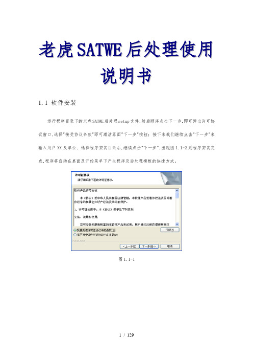
老虎S A T W E后处理使用说明书1.1软件安装运行程序目录下的老虎SATWE后处理setup文件,然后顺序点击下一步,即可弹出许可协议窗口,选择"接受协议条款"即可激活界面"下一步"按钮;接下来我们继续点击"下一步"来输入用户XX及单位、选择程序安装目录后,继续点击"下一步",出现图1.1-2则程序安装完成,程序将自动在桌面及开始菜单下产生程序及后处理模板的快捷方式。
图1.1-1图1.1-2提示:软件使用过程中请用户不要拔除加密锁,如用加密锁启动后处理后,拔掉加密锁程序将变成试用版本;即使再插上加密锁,程序仍为试用版本;需先退出,或再启动另一后处理程序进程方可恢复程序为正式版本;另外:在程序读加密锁时拔出也易造成加密锁的损坏,在此提请用户注意!1.2软件运行软件安装结束,下面我们可以开始工作了,在这里需要提醒用户的是,本软件运行前应先完整的运行PKPM系列软件的SATWE程序,然后进入程序的文件菜单点击"导入SATWE模型及计算结果"〔图1.2-1〕,弹出目录选择菜单〔图1.2-2〕〔程序运行默认进入此选择菜单〕,选择SATWE工作目录中的WPJ.SAT,程序将自动读取SATWE相关的结果文件,如果用户指定的读取目录非SATWE计算目录,而是"后处理目录"下的"SATWE结果备份"目录,为防止用户错误使用SATWE结果文件,程序会给出<图1.2-3>提示。
图1.2-1图1.2-2图1.2-3➢保存默认设置:为方便用户保存"老虎SATWE后处理"工作设置,增加菜单"保存设置到后处理安装目录",点取该菜单程序自动将GBCJOB.IN〔包含所有可以改动的设置〕文件保存至后处理安装目录,以后开启程序,自动加载此设置。
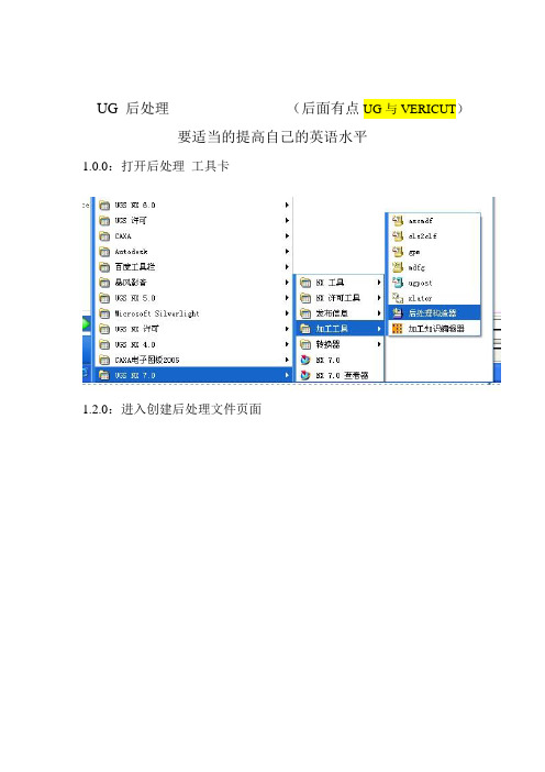
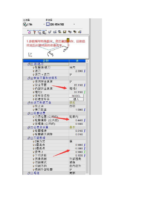
UG 后处理(后面有点UG与VERICUT)要适当的提高自己的英语水平1.0.0:打开后处理工具卡1.2.0:进入创建后处理文件页面1.2.1 创建一个新的后处理文件这里输入文件名(英文)此区域Inches 英制单位Millimeters 公制设定此区域轴选项3-轴4-轴或5轴这里只讲解3轴通用设定此区域为机床类型设定Generic 通用的Library 浏览自带机床User’s 用户自定义此区域描述你的后处理单只能输入英文选择完自己需要的格式后处理单击OK 进入下一步这一选项进行修改你的程序头程序尾中间换刀程序衔接道具号道具属性显示的添加进行讲解此选项为程序头选项此选项为增加程序条命令点击它可以拖入程序条就像这样这里的垃圾桶通样你不想要的此条可以删除下面讲解通用的编程设置下面图片是默认的设置此选项为N码关闭此选项为N码开启一般都是把这条此选项需要更改改成你需要的G40 G49 G80 G90既可单击这条词条就可修改进入下一画面把不需要的拖入垃圾桶通过此选项里的代码你可以找到你想要的改好后点击OK既可安全起见最好加入个Z轴回零命令拉入一个词条框添加一个新的词条框如果你想把词条框放在哪个词条框的周围只要看好词条对应放置位置变白既可松掉鼠标下面进入新词条选项里点击这里可以加入你要的词条而我们需要的是 G00 G91 G28 Z0 命令可以用文本形式输入就是这里选择第二个选项“TEXT”文本点击 Add word 拉入这个区域同样变白放置输入你要的文本G00 G91 G28 ZO 点击OK 既可程序头设定完成就是这个效果看下图如果需要加入O号下面编辑你的换刀过程点击中文意思就是操作开始步骤在这里你可以加入你需要的道具信息 N号的开关 M8 M9的开关设置 G43H00等设置下面先讲解 N号的加入加入N号我们只需要拉两个 N号开关词条就可以选择这一选项拉到上面是N号开然后拉入在下面既可下面加入刀具信息找到这个选项操作员消息拉入 N号关后面输入命令MOM_output_literal “( 刀具名称:$mom_tool_name )”MOM_output_literal “( 刀具直径:$mom_tool_diameter )”MOM_output_literal “( 刀具R角半径:$mom_tool_corner_radius )”想要哪个信息就输入哪行如果要两个以上就飞边拉入词条输入这项编辑完毕单击蓝色的区域机床控制 Machine Control 进入一下界面我们只要在G43后加上M8既可完成此项设定然后点击进程动作设定我们只需要修改中间的那个 G02 G03的进入下一页面该为Vector-Arc Start to Center 修改后OK 推出不改出程序带R的带圆的程序就是乱做一团。
已经在群里发共享后处理文件和测试后处理文件,还有测试文档,还有不明白的地方可以留言,有空就帮解答。
注意的地方:
1.所有的变量名都属于某一个模块,放到对应的模块下才能正确显示。
如果找不到这个模块,就把上面黑体字和下面变量一起复制进去。
(因为开源后处理有部分不常用的地方都删除了。
测试后处理Testgpp2包含所有完整的模块)
2.模块内的变量名如果想在全局使用,要在顶部自定义全局变量=局部变量,然后才能在任何地方输出。
比如有的程序头变量在程序尾部就无法输出,要定于为全局变量才能输出。
3.刀具信息是单独的一个模块,里面输出的是一个数组,里面有所有的刀具参数。
4.如果还有不明白的地方,可以在群里留言,有空就回复咯。

三维网:为中国机械制造行业提供全方位的信息资讯!FTP 搜索 | 下载论坛附件流量兑换 | 在线充值 | QQ 客服1| QQ 客服2 | 繁體中文791744496 我的帖子 短消息 论坛任务 个人中心 退出• • 论坛 • 站内搜索 • 论坛设施 • FTP 服务中心 • 百宝箱 • 导航 • 帮助 • 默认风格 • 三维蓝 • 蓝 •newyear三维网技术论坛» 『Siemens NX 技术交流区』 » 『NX CAM 区』 » UG 后处理批处理教程--问题 UG 、Pro/E 最新全套视频教程(34DVD )返回列表 下一主题 ›› ‹‹ 上一主题 回复 发帖[讨论] UG后处理批处理教程--问题 zzlok三维学徒1#打印 字体大小: t T发表于 2010-3-14 18:35 |新手如何挣论坛积分,提高权限 | 只看该作者[讨论] UG 后处理批处理教程--问题本帖最后由 zzlok 于 2010-3-14 18:36 编辑帖子86 积分99 流量1502 K 注册时间2009-10-28UG后处理批处理教程1:先打开你的后处理*.TCL文件找到SETMOM_SYS_GROUP_OUTPUT 设为ON2:打开你的UG安装目录下NX3.0\MACH\RESOURCE\postprocessor\下的UGPOST_BASE.TCL文件找到set grp_ptp_name"${mom_output_file_basename}_${group_name_lowercase}${o utput_extn}"改成set grp_ptp_name"${group_name_lowercase}${output_extn}"3:找到 proc mom_start_of_group下面的 if {$mom_sys_ptp_output == "ON"} {MOM_open_output_file $ptp_file_name 改成 if {$mom_sys_ptp_output == "ON"} {MOM_remove_file $ptp_file_name4:继续找到 proc mom_end_of_group下面的 if {$mom_sys_ptp_output == "ON"} {MOM_open_output_file $ptp_file_name 改成 if{$mom_sys_ptp_output == "ON"}{MOM_remove_file $ptp_file_name5:保存 UGPOST_BASE.TCL文件!6 进入UG加工模块,点最上面的NC PROGRAM组上面进行后处理就OK了!这个教程我按照方法修改好几次了可是总是出现这一个问题 ------所以我还不知道这个教程具体是做什么的为什么我按照方法修改这么会出现错误时怎么回事啊!谢谢大家3.jpg (26.83 KB)2.jpg (61.49 KB)收藏分享评分UG.PowerMILL.MasterCAM,SolidWorks工厂实战视频教程回复引用订阅报告道具TOPotnt版主帖子845积分10022流量2745769 K注册时间2008-6-152#发表于 2010-3-14 21:30 |新手如何挣论坛积分,提高权限 | 只看该作者本帖最后由 otnt 于 2010-3-14 21:49 编辑调整成类似如图节点格式,然后就可以了输出时选择program节点,当然也可以选择其他节点(具体区别自己可以试一下)1.jpg (28.67 KB)借我三千虎贲,复我浩荡中华;剑指天山西,马踏黑海北;贝加尔湖面张弓,库页岛上赏雪;中南半岛访古,东京废墟祭祖;汉旗指处,望尘逃遁!敢犯中华者,虽远必诛!!UG.PowerMILL.MasterCAM,SolidWorks工厂实战视频教程回复引用报告道具TOPzzlok3#三维学徒帖子86 积分99 流量 1502 K 注册时间 2009-10-28发表于 2010-3-18 20:56 |新手如何挣论坛积分,提高权限 | 只看该作者2# otnt能具体说说嘛 没明白节点是什么意思 不好意思UG.PowerMILL.MasterCAM,SolidWorks 工厂实战视频教程回复 引用报告 道具TOPotnt版主帖子 845 积分 10022 流量4#发表于 2010-3-18 23:46 |新手如何挣论坛积分,提高权限 | 只看该作者上传后置及文件借我三千虎贲,复我浩荡中华;剑指天山西,马踏黑海北;贝加尔湖面张弓,库页岛上赏雪;中南半岛访古,东京废墟祭祖;汉旗指处,望尘逃遁!敢犯中华者,虽远必诛!!UG.PowerMILL.MasterCAM,SolidWorks 工厂实战视频教程2745769 K 注册时间 2008-6-15回复 引用报告 道具 TOPhfly2002三维工程师帖子 669 积分 1473 流量 784041 K 注册时间 2006-9-145#发表于 2010-4-17 18:50 |新手如何挣论坛积分,提高权限 | 只看该作者 本帖最后由 hfly2002 于 2010-4-17 18:52 编辑我的也不行 能帮我改下吗 ? 我的文件没PUI 的Sim810d_post.rar (18.65 KB)UG.PowerMILL.MasterCAM,SolidWorks 工厂实战视频教程回复 引用报告 道具 TOPxuelang1161166#发表于 2010-4-19 18:49 |新手如何挣论坛积分,提高权限 | 只看该作者学习一下. 试试看三维总工帖子 717 积分 1561 流量 2249521K 注册时间 2007-4-2UG.PowerMILL.MasterCAM,SolidWorks 工厂实战视频教程回复 引用报告 道具TOPotnt版主帖子 845 积分 10022 流量7#发表于 2010-4-20 23:25 |新手如何挣论坛积分,提高权限 | 只看该作者5# hfly2002在没有pui 文件的时候,调试后置就需要将TCL 文件中 MOM_set_debug_mode 设为 ON 就可以在NX 中调试了调试就会发现提示如图,是输出刀具信息有问题输出刀具信息改到换刀模块处。
2009.11.2 CDAJ-China 技术部引言引言 本手册以Tutorial为蓝本,简单模型为范例,重点讲述了GT-POWER 建模的具体操作。
具体内容分为五部份:绪论第一章单缸汽油机模式第二章单缸柴油机模式第三章四缸汽油机模式第四章后处理详细模型及其它诸多功能未载入本手册,敬请参阅随机文档Tutorial 和Example 。
2009 11.2 绪论绪论 对于GT-SUITE软件来说,它们处于同一个操作平台和同一个后处理器,所以对于它们的操作和后处理是相同的。
操作平台称之为:GT-ISE,对于不同的软件模块来说,它们的操作环境与下图相差不大: 对于不同的GT模块,上图左边的数据库文件有差异。
导航图主要用于当模型过大时,便于显示不同区域。
模型管理器中所有的组成是建模必须的模板。
建模区域用来定义不同零件之间的联接关系。
数据库导航图模型管理模型区域第一章第一章单缸汽油机模拟单缸汽油机模拟 本章主要讲述GT-POWER中简单模型的建模、静态分析和后处理显示。
输入参数的具体含义请参照GT-POWER的用户手册和在线帮助。
1.1 启动GT-ISE : 鼠标双击GT-ISE 图标,或者 启动菜单 1.2 创建新模型 1.2.1 鼠标选择FILE/NEW, 或者鼠标单击图标第一章第一章单缸汽油机模拟单缸汽油机模拟 1.2.2 按右图选择导入空模板· 1.2.3 将模型另存为POWERtut1.gtm 1.3 加载模板 1.3.1 调出模板库。
选择Window/Tile with template library 或者鼠标单击图标第一章第一章单缸汽油机模拟单缸汽油机模拟 1.3.2 加载模板鼠标拖动,或复制粘贴,加载右图所示模板 1.4 定义对象 1.4.1 进口环境 双击上图右边的 EndEnvironment模板, 输入右图所示的主页面参数点击可进入在线帮助第一章第一章单缸汽油机模拟单缸汽油机模拟 注:对于每个部件通过上述方式获得在线帮助,可以得到每个参数的意义说明。
MasterCAM X3 软件的后置处理文件优化及其设定方法Mastercam 是一套应用广泛的CAD/CAM/CAE软件包,它采用图形交互式自动编程方法实现NC 程序的编制。
交互式编程是一种人机对话的编程方法,编程人员根据屏幕提示的内容,反复与计算机对话,选择菜单目录或回答计算机的提问,直至将所有问题回答完毕,系统即可自动生成NC程序。
NC程序的自动产生是受软件的后置处理功能控制的,不同的加工模块(如车削、铣削和线切割等) 和不同的数控系统对应不同的后处理文件。
软件当前使用哪一个后处理文件,是在软件安装时设定的,而在具体应用软件进行编程之前,一般还需对当前的后处理文件进行必要的修改和优化,以使其符合系统要求和使用者的编程习惯。
有些用户在使用软件时,由于不了解情况,没有对后处理文件进行修改,导致生成的NC程序中某些固定的地方经常出现一些多余的内容,或者总是漏掉某些词句。
解决这类问题,一般都需要在将程序传入数控机床之前,对程序进行手工修改,如果没有全部更正,则可能造成事故。
例如,在数控编程中可以去掉程序行号,以控制程序文件大小,便于文件的快速上传。
又如,更改某些不同系统的不同程序代码,或限定主轴和进给速度的最大与最小极限速度。
再如,确定立式和卧式机床型号等。
本文介绍了Mastercam 后处理文件的内容以及修改和设置的方法,供有关人员参考。
一、启动Mastercam 软件的修改文件以铣削为例,在安装的MaterCAM根目录下,采用记事本打开MPFAN.pst 文件(位置为“ D:\mcamx\mill\Posts\MPFAN. pst”)。
图1所示即为该文件。
后置处理文件简称后处理文件,是一种可以由用户以回答问题的形式自行修改的文件,其扩展名为“.PST”。
在应用Mastercam软件的自动编程功能之前,必须先对这个文件进行编辑,才能在执行后处理程序时产生符合某种控制器需要和使用者习惯的NC程序,也就是说,后处理程序可以将一种控制器的NC程序,定义成该控制器所使用的格式。
GT-SUITEGT-POST TutorialsVERSION 7.5byGamma TechnologiesCopyright 2015 © Gamma Technologies, Inc. All rights reserved.All information contained in this manual is confidential and cannot be reproduced or transmitted in any form or by any means, electronic or mechanical, for any purpose, without the express written permission of Gamma Technologies, Inc.GTI Information GTI SUPPORT•TELEPHONE: (630) 325-5848•FAX: (630) 325-5849•E-MAIL: support@•Web Address: •Address: 601 Oakmont Lane, Suite 220Westmont, IL 60559USATelephone Support Hours8:00 A.M. to 5:30 P.M. Central Time Monday – FridayTable of ContentsTABLE OF CONTENTSTUTORIAL 1:General Use of GT-POST (1)1.1Introduction (1)1.2Set-up (2)1.3Viewing a Plot (2)1.4Customizing a Plot (4)1.5Creating Multiple Plots (8)1.6Customizing Multiple Plots (8)1.7Entering Data Manually (10)1.8Importing Data from Text Files (11)1.9Importing Data from Excel (13)1.10Comparing Two Different Models (14)1.11Creating Tables (16)1.12Viewing Instantaneous Plots (17)1.13Combining Cases of Instantaneous Plots (19)1.14Other Plotting Options (21)1.15RLT Contour Map (22)1.16Animated Displays (23)1.17Transient Example (24)1.18Conclusions (26)TUTORIAL 1: General Use of GT-POSTThis tutorial has been prepared to teach a new user about GT-POST. GT-POST is a plotting and data-handling tool used by GT-SUITE. Several uses of GT-POST are shown in this tutorial through consecutive sections analyzing the results of a basic engine simulation. Although this tutorial focuses on post-processing results of engine simulation models, the use of GT-POST is identical with all applications and thus this tutorial will be beneficial for all users of GT-SUITE software.1.1 IntroductionSeveral methods for analyzing simulation results are offered in GT-POST. Below is a list of the different post-processing formats in GT-POST.Instantaneous Plots: These plots are of values with respect to the crank angle for GT-POWER over the last cycle of each case. These are very useful for looking at how things change over one cycle of the engine. For example, it is helpful to look at how the mass flow rate or lift of the valves varies with the crank angle.Case RLT Plots:These plots are made from all the RLT (results) data gathered for the various part variables from the model simulation. They are very useful for analyzing results of simulations with several cases where a specific variable changes for each case. The RLT results stored are steady-state periodic simulations where the results are averaged over the last cycle of each case. For example, comparing a varying engine speed over several cases with the volumetric efficiency, power, torque, or many other variables will produce important performance plots.Time RLT Plots: These plots are for transient simulations since they are cycle-averaged quantities that vary with time during a transient event. If, for example, the engine is varying speeds with respect to time throughout the simulation, then these plots will show the effect of this variation on the engine measurements.RLT Contour Map:This is a visual representation of the Case RLT data, using color contours to represent values. The contoured data is then overlaid on the model display to show parameter variations everywhere in the model. A global view of the model is given for each case. This can be useful for trying to understand how conditions vary in different areas of the engine.Animated Contour Map: This is a feature that allows the user to view what is happening throughout the cycle of the entire engine model. It is much like the RLT Contour Map since it shows the entire engine and uses color-contours to display the values. However it shows the Time RLTs for a complete cycle. This gives very specific visual results; for example displaying the pressure at many instants in time throughout the cycle can help one determine when certain parts are reaching their maximum pressure. Tables: Tables can be created to view Case RLT data collected and save it for future reference. Many tables of data are created by GT-POST automatically in the GX file; however, many other tables can be created with only requested data.1.2 Set-upBefore the post-processing, a model must be run to obtain simulation results. From GT-ISE, open themodel file SI_4cyl_Basic.gtm located in %GTIHOME%\vX.X.0\examples\Engine_1D_Gas_Exchange_Combustion\Gasoline\SI_4cyl_Basicfolder and run the example model. This four-cylinder engine will be used to generate the results used forpost-processing.Once the simulation is finished, two of the several output files created are called SI_4cyl_Basic.gx andSI_4cyl_Basic.gdt. These are the primary files used by GT-POST, and they contain all of the data fromthe simulation. Open GT-POST by clicking the GT-POST icon from the GT-ISE toolbar, or byselecting Run/Open GT Post. Select the SI_4cyl_Basic.gx file if it is not automatically selected, andclick Open. This will open a GT-POST window, which will look similar to Figure 1 shown below.Note: Some figures may appear slightly different from your screen due to desktop settings or otherchanges to the GT-POST interface.Figure 1: The GT-POST window1.3 Viewing a PlotOnce the SI_4cyl_Basic.gx file has been opened, all of the results are available to be viewed and/or customized.1.Click on the CaseRLT tab in the SI_4cyl_Basic.gx window as shown in Figure 2, and theCaseRLT plot names will be displayed in a tree format.2.Scroll down to the EngineCrankTrain group, and expand to the Flow data for the engine by firstclicking on the plus symbol to the left of the EngineCrankTrain group. Next, expand the engine data by clicking on the plus symbol to the left of the Engine part. Then, expand the Flow folder.The window should then look similar to Figure 2 below.CaseRLT TabFigure 2: The Case RLT tree format.3.Right-click on the first data set called Volumetric Efficiency, Air and select View. Pressing F4on the keyboard will also display the highlighted data set. The plot should appear in the default settings similar to Figure 3. The plot window can be moved and re-sized if necessary.Note that on this plot, the X-axis has been set up to display Engine Speed (RPM) instead of case number, which is the default. This can be done before the simulation is run in GT-ISE by opening the Setup menu and selecting Output Setup. Then, in the GT-POST_Setup tab, use the Value Selector to change X-Axis RLT for Case Sweep Plots to the Engine Speed RLT, or any other RLT variable that is desired.Figure 3: A plot of the volumetric efficiency for each engine speed.1.4 Customizing a PlotBefore beginning to customize the plot, a new file that must be created so the plot properties can be saved. This file is called a User Plots File or Report File (GU). The Report File does not store the simulation data explicitly; it is linked to the results data *.gdt file implicitly. The plots created in the Report File will be updated if the simulation data changes.1.Select the New Report File (GU) toolbar button and an empty Report File window will appearas shown in Figure 4.2.Change the name to correspond with the GX file by choosing Save As in the File menu, and thenname the file "SI_4cyl.gu".New Report windowFigure 4: The new Report File icon and window.Plot properties can be changed in the GX file, but these changes cannot be saved. Therefore, plots and plotting formats are usually customized in a Report File (GU).A standard initial group named New Group is in the Report File so that a plot can be immediately copied into the file.1.Change the name of this New Group to RLT Plots by double-clicking on the name to open theproperties window and changing the Name, or by right-clicking and selecting Rename.2.Highlight and drag the Volumetric Efficiency, Air CaseRLT plot from the GX file into the RLTPlots group in the SI_4cyl.gu file.It is important to note that the Report File has four levels in the tree format: title, group, plot, and data level. These levels are labeled in Figure 5, and they can be expanded the same way as in the GX file. They are important since some properties can only be changed from certain levels. It is also important to know that a change made at a higher level will affect the sub-levels below. Changes can be made to a given level by right-clicking on the level in the tree and selecting Properties, or by right-clicking on the plot and then selecting the properties option for the appropriate level.Figure 5: Labeled levels in the SI_4cyl.gu file.First, make the changes to the axis and format of the plot in the following manner.1. Right-click on the plot or the Plot level in the tree and select Plot Properties . From thiswindow, the X-axis, Y-Axis, and general plot format can be changed.2. To add minor divisions on the X-axis, select Scale from the X-axis tree. The Minor Divisionsbox specifies the number of minor divisions per major division. In the Minor Divisions box, put a 2 to place a tick-mark on the X-axis at 500 RPM intervals.3. To change the Grid Lines for the Y-axis, click on Grid in the Y-axistree, and select short-dashas the Grid Lines type. Also to use easy to read numbers for the axis, set theminimum and maximum for the range to be Auto under the Scale .4. The axis labels can be changed from Labels .5. Press the OK button to save the changes to the Plot Properties.Now, change the way the data points are shown.1. Right-click on the SI_4cyl data level and choose Properties . The properties window can also bereached by right-clicking on the plot and selecting Data Properties and SI_4cyl .2. In the Display branch of the tree, change the Symbols: Style to increment to add the datamarkers. The markers will be selected according to the rules specified in Tools > Options > Plot Auto Increment Settings . Increment rules for the line type and color can also be changed.3. The line thickness, type, color, and data symbols can also be changed. Mathematical operationscan also be performed from the Data Properties window.4. Press the OK button to save the changes to the Data Properties.Re-generate the plot by selecting the plot and pressing F4 to view. The plot should look similar to Figure 6 after all of the changes have been made.Title LevelGroup Level Plot LevelData LevelFigure 6: The formatted plot of volumetric efficiency for each engine speed.In GT-POST, the current plot view is called the Live View, and is represented by the symbol in the tab at the bottom of the plot window. Display properties of a Live View plot can be altered both from right-clicking in the plot window and by right-clicking on the plot or data name in the Report File (GU) window. When a new View command is issued for a different plot, the default GT-POST behavior is to take a Snapshot of the current plot and create a new Live View plot with the data requested by the user.A Snapshot, represented by the symbol , is a plot not linked to a GX or Report File and is stored in short term memory. The Snapshot can only be altered from property changes made in the plot window.A Live View plot is directly linked to the GX or Report File, so if a simulation is re-run and results change the Live View plot will be updated accordingly. One further note is that changes made to the plot in a Live View window are saved when the Live View is switched, whereas changes made to a Snapshot are lost if the Snapshot is closed. Snapshots can also be pinned to the plot window using the Pin Snapshot button to prevent them from being easily closed.To change the default behavior for Snapshot creation, select Tools/Options… and go to the Plot/Table Viewing tab. Uncheck the box next to “Automatically create snapshot when plotting” if Snapshot creation is not desired. To manually create a snapshot when this option is turned off, right-click on thetab at the bottom of the plot window and select Make Snapshot.1.5 Creating Multiple PlotsTo create multiple plots of result variables at once, use the RLT Plots macro button. This macro can also be accessed by selecting Macro/RLT Plots…. In this section, plots of the Brake Power (HP), Brake Mean Effective Pressure (BMEP), and Brake Specific Fuel Consumption (BSFC) vs. the Engine Speed will be created.1.Click on the SI_4cyl_Basic.gx window to make sure that it is activated, because the macros canonly be used if the GX file is activated. Click on the RLT Plots macro button on the toolbar or in the Macro menu.2.Choose the Case RLT RLT Type, and the XY Scatter Plot Plot Type, and click Next.3.Find and select the Engine Speed RLT (cycle average) in the Performance Folder of theEngineCrankTrain component.4.Click on the variable while the cursor is in the X column. This will be the X variable for allfurther plots selected.5.Move the cursor to the Y1 column / Plot1 row in the top window, and then select the followingvariables: Brake Power (HP) (in the Torque-Power Folder), BMEP (in the Performance Folder), and BSFC (in the Performance Folder).6.Once the Data tab has the same RLTs as Figure 7, select Next. In the Dataset Label andDisplay Options, select “Model Name” and unselect Part Name, RLT Name, and Constraint RLT. Make sure that the Document Name is SI_4cyl.gu, and click Finish to create the plots.These three plots should now be listed in the SI_4cyl.gu file.Figure 7: The Plot RLT Macro window.1.6 Customizing Multiple PlotsThe tree system enables multiple plots to be customized simultaneously. To change the properties for several plots in a group, change the Children Properties for that particular group. In this section, the newly created plots will be formatted like the Volumetric Efficiency plot.1.Right-click on the RLT Plots group level in the SI_4cyl.gu window, and select ChildrenProperties.2.Select the Plot option for the Property Type, and click Next.3.To only change the values for certain plots, uncheck the box next to that tree item in the SelectTree Elements window (Figure 8). Since all of the plots will be formatted the same, leave all of the boxes checked and click Next.Figure 8: Select Tree Element Window4.Go to the Scale branch of the X-Axis tree, and then the Minor Divisions box. Change thenumber in the box to 2; this divides the Major Intervals into 500 RPM intervals.5.To change the Grid Lines on the Y-axis, click on the Grid branch of the Y-axis tree, and selectshort-dash as the Grid Line type. Also, to use easy to read numbers for the axis, go to the Scale branch select the minimum and maximum for the range to be Auto. Click Finish to display the updated plots.6.To change the symbol type, re-open the Children Properties window by right-clicking on theRLT Plots group level in the SI_4cyl.gu window.7.In the Property Type window, change the Property type to Data, and click Next to advance tothe Select Tree Elements window. Ensure that the boxes next to each plot are checked, and click Next. In the Property Modification window, choose the Display tree branch and change the Symbols: Style to increment.8.Click Finish to display the formatted plots.All 4 of the graphs in the RLT Plots SI_4cyl.gu file will now have the same properties. Flip through the 4 plots by using the page left/page right buttons on the toolbar. To view all 4 plots on the same screen, select the RLT Plots group, and then right-click and select Properties. Then select 2x2from the dropdown next to the Layout: option. Click OK and the plot screen should look similar to Figure 9. Tochange back to 1 plot per page, change the Layout dropdown back to 1x1.Figure 9: The CaseRLT plots displayed in a 2x2 array.1.7 Entering Data ManuallyTabulated data can be added to a GT-POST plot. Data entered manually is explicitly stored in the Report File (GU). Sample data is provided for the Volumetric Efficiency, and is shown in Table 1 below.Table 1: Sample Volumetric Efficiency DataEngine Speed (RPM) Volumetric Efficiency6000 0.96215500 1.02285000 1.01194500 1.00214000 0.97183500 0.91063000 0.90872500 0.86371.Enter this sample data manually by right clicking on the Volumetric Efficiency Plot level, andthen selecting Add Data.2.Select Explicit for the Data Source and click Next.3.Enter the Data Name: "Sample", and then click Finish. For other data sets, the units can bechanged to convert the entered data to match the simulation units.4.Enter the data from Table 1, and select OK. The column titles do not need to be entered in toGT-POST.5.Select the Volumetric Efficiency plot from the tree and press F4(if Automatic view is notselected) to view the plot.The sample data will be plotted on the same graph as the simulation output data for Volumetric Efficiency. By default, the "Sample" set will be the first data set in the plot. The line color is automatically specified by the data set order; therefore it should be easy to differentiate between the data sets. The data set order can be changed by dragging the icon for the set to the desired position in the Report window tree diagram. Properties of each data set can be also be specified individually.1.Right-click on the Sample data level under the Volumetric Efficiency plot level in the Report File(GU) window, and select Properties.2.In the Display branch of the tree, change the Symbols:Style to increment and press the OKbutton to add the data markers.The formatted plot should look similar to Figure 10.Figure 10: The plot of the sample and simulation data for Volumetric Efficiency.1.8 Importing Data from Text FilesData contained in text files can also be imported into GT-POST. Sample data for the Brake Power (HP) has been provided in the Experiment.txt file located in the %GTIHOME%\v7.x.0\tutorials\Graphical_Applications\GTpost\01-GeneralUse\ folder. Open the file Experiment.txt in a text editor to ensure that it matches Figure 11.Figure 11: Text File with Experimental DataImport the experimental data for the Brake Power (HP) contained in this text file by doing the following:1.Right-click on the Brake Power (HP) plot level and select Add Data.2.Select Ascii for the Data Source, find the file named Experiment.txt by using the Browse button,and click Next.3.Configure the Delimiters to only be Tab, and select Next.4.Because the text file has a title row, only the column titles and data need to be imported.Highlight the row containing the Engine Speed and Brake Power labels and move the data to the right window by pressing the button. Make sure the "Take Whole Column" checkbox is selected to move all of the data.5.In the right window, change the first row from Data to Label. The first two rows of the importedinformation can be specified as Data, Label, or Unit to match the format of the file. The rest of the rows are assumed to be Data.6.Select Next to review the Data Options. ASCII data may be imported implicitly, meaning that ifthe .txt file is updated with new data the GT-POST plot will be updated accordingly, or explicitly, which makes a copy of the data in the .txt file at the time and stores the data in the Report File (GU).7.Select Finish to create the data set.8.Drag the Brake Power (HP) data set to the second position in the Brake Power (HP) plot level inthe Report File window.9.Select Properties after right clicking on the Brake Power (HP) data level.10.In the Display branch of the tree, change the Symbols:Style to increment to add the datamarkers. The plot should look similar to Figure 12.Figure 12: Plot of Experimental & Simulation Data for Brake Power (HP)1.9 Importing Data from ExcelData contained in excel files can also be imported into GT-POST. Sample data for the Brake Mean Effective Pressure (BMEP) has been provided in the ExperimentData.xls file located in the %GTIHOME%\v7.x.0\tutorials\Graphical_Applications\GTpost\01-GeneralUse\folder. The steps for importing an Excel file follow similar steps to importing an Ascii file.1.Right-click on the Brake Mean Effective Pressure plot level and select Add Data.2.Select Excel for the Data Source, find the file named ExperimentData.xls by using the Browsebutton, and then click Next.3.To import the entire data set, select the top row of the spreadsheet. Move the information to theright window by pressing the button. Make sure the "Take Whole Column" checkbox is selected to move all of the data.4.In the right window, select the "Label" and "Unit" option for rows 1 and 2, respectively.5.Select Next to review the Data Options. Excel data may be imported implicitly, meaning that ifthe .xls file is updated with new data the GT-POST plot will be updated accordingly, or explicitly, which makes a copy of the data in the .xls file at the time and stores the data in the Report File (GU).6.Select Finish to create the plot.7.Arrange the data and format the dataset like the previous plots. The plot should be similar toFigure 13.Figure 13: Plot of Experimental & Simulation Data for BMEPSince we do not yet have experimental data for the BSFC, we can unselect the check mark for that plot. Now plot all 3 plots by highlighting the group 'RLT Plots' and pressing F4.1.10 Comparing Two Different ModelsAnother model has been created to illustrate the method for comparing similar GT-ISE models. The new model is based on the SI_4cyl_Basic.gtm model used previously; the intake and exhaust geometry has been changed. The intake runner length has been increased from 320 mm to 380 mm, and the exhaust runner length has been increased from 250 mm to 300 mm. This new model is titled SI_4cyl_long.gtm and is located in the %GTIHOME%\v7.x.0\tutorials\Graphical_Applications\GTpost\01-GeneralUse\ folder.It is important to know that once a Report File (GU) is built for a model, the Report File does not have to be built again for a second similar model. If changes are made to the model and the results need to be compared, this can be done by adding the similar model information to the Report File to create new plots. The pointers used to specify the data for the first model are used for the second model.For convenience, the SI_4cyl_long.gtm model has already been run. The files SI_4cyl_long.gx and SI_4cyl_long.gdt are contained in the same folder as the model, and the data will be added to the current Report File.1.Right-click on the RLT Plots group level, and select Change Data Source.2.In the Select Operation Window, select Copy for the Data Operation option and File Namefor the Search By option. This means you will be copying the pointers originally used for SI_4cyl.gdt. Click Next.3.Select SI_4cyl.gdt as the File to copy and browse to find SI_4cyl_long.gdt in the above directoryas the File to replace with.4.Click Next.5.Under the Data Label Settings, select New and enter SI_4cyl_long, and then select Finish.Now all the plots in the RLT Plots group will have 3 data sets each except for the BSFC plot with 2 data sets. With the use of Change Data Source, all of the pointers referring to SI_4cyl.gdt were copied and changed to point to SI_4cyl_long.gdt. To view only the new data, use the Data Selection Wizard. The Data Selection Wizard can be used to easily change the source data displayed for multiple plots.1.Select only the data sets belonging to SI_4cyl_long by right clicking on the RLT Plots group andselecting Turn On/Off Datasets to launch the Data Selection Wizard.2.In the Select Datasets window, uncheck the boxes next to the files SI_4cyl.gdt, Experiment.txt,and ExperimentData.xls.3.Select Finish to exit the wizard.4.Because explicit data is not affected by the Data Selection Wizard, uncheck the box next to theSample dataset for the Volumetric Efficiency plot.5.View the plots for the new data.6.Then re-display the data from the first model, by using the Data Selection Wizard again, andselect/check the boxes for SI_4cyl.gdt, Experiment.txt, and ExperimentData.xls.For a direct comparison between the two models, the Plot/Table Math Operations macro can be used to plot the percent difference in Brake Power between the SI_4cyl and the SI_4cyl_long simulations.1.Activate the SI_4cyl.gu file by clicking on the Report File (GU) window.2.Click on the Plot/Table Math Operation macro button in the GT-POST toolbar or select itfrom the Macro menu.3.Under the Select operation type menu, Select Percent Difference and press Next.4.Expand the RLT Plots tree to display the plots. Expand the Brake Power plot, and drag theSI_4cyl_long data set down into the Build math dataset(s) pane. It will be assigned as the Y1 data set.5.Next, drag the SI_4cyl_Basic set down. It will be assigned as the Y2 data set. Click Next.6.Change the User Group to <Create New Group> and press Finish.The plot should be similar to Figure 14.Figure 14: Plot of the percent difference in Brake Power between SI_4cyl_long and SI_4cyl.1.11 Creating TablesTables of simulation data can also be created using GT-POST. A table containing the Volumetric Efficiency, Brake Power, Brake Mean Effective Pressure, and Brake Specific Fuel Consumption can be created for data storage in the following manner.1.Activate the SI_4cyl_Basic.gx file, and click on the RLT Tables icon in the toolbar or fromthe Macro menu.2.From the Performance folder in the EngineCrankTrain Component, select the data that isrequired to be included in the table by clicking on the RLT variable names: Engine Speed, Volumetric Efficiency (in Flow folder), Brake Power (HP) (in Torque/Power folder), Brake Mean Effective Pressure, and Brake Specific Fuel Consumption. The variable table should look like Figure 15.3.Click OK to create the table.Figure 15: The RLT variable table in the RLT Tables macro.Once this table is created, it will be placed under the Tables tab in the SI_4cyl.gu file in the new group. The name of the table needs to be changed from the default "New Report Table1" to "RLT Data" by right-clicking on the name and choosing Rename. The table should look like Figure 16.Figure 16: Table of RLT Data1.12 Viewing Instantaneous PlotsThe Instantaneous Plots, which plot variables with respect to Crank Angle or Time for GT-POWER, will be used to analyze the results in the valves. The Part Data Combine macro can be used to compare similar instantaneous data from the same part types. For this example, the mass flow rate from the intake and exhaust valves will be compared for a given crank angle.1.Activate the SI_4cyl_Basic.gx window, and then select the Plot Data Combine toolbar buttonor use the Macro menu.2.In the left pane, select the mass flow rate data from one of the exhaust valves(ValveCamConn:ExVal1A or B).3.In the middle pane, select the mass flow from the matching intake valve.4.In the right pane, select all the cases.5.Finally change the User Group to <Create New Group>. The dialog should look like Figure 17.6.Now, press OK.7.In the Report File (.gu) window, rename the newly created group as "Instantaneous Plots".Figure 17: The Plot Data Combine window.The plots should look similar to Figure 18 for the mass flow rate of the intake and exhaust valves.。