Kernel休眠与唤醒综述
- 格式:docx
- 大小:26.94 KB
- 文档页数:12
wakeup的用法总结一、wakeup技术简介wakeup是一种在计算机科学领域常用的技术,主要用于唤醒处于睡眠状态的设备或应用程序。
该技术使得设备能够在特定条件下自动从休眠状态中恢复,从而提高工作效率并节省能源。
二、wakeup技术的应用场景1. 移动设备的唤醒随着智能手机等移动设备的普及,wakeup技术被广泛应用于此类设备上。
当用户长时间未操作设备时,系统会进入休眠状态以降低功耗。
然而,在某些情况下,需要即时接收通知或推送消息等重要信息。
这时,wakeup技术可以实现通过网络API或定时器等方式唤醒设备,并进行相应的操作。
2. 物联网领域中的远程唤醒物联网是近年来兴起的一个概念,指通过互联网将各种物理对象连接起来形成一个巨大的智能网络。
在物联网中,很多设备会处于低功耗休眠状态以节约电量和延长使用寿命。
但是,在某些场景下需要迅速与这些设备进行通信、控制或监测等操作。
wakeup技术可以满足这些需求,通过对设备进行唤醒,实现远程操作。
三、wakeup技术的工作原理wakeup技术的实现主要分为硬件层和软件层两个方面。
1. 硬件层在硬件层面,常见的唤醒方式包括外部中断、定时器和电平触发等。
外部中断指的是通过外部设备或传感器发送的信号来唤醒设备。
定时器则是根据预设的时间间隔周期性地唤醒设备。
电平触发则是基于某个特定信号值改变来触发唤醒操作。
2. 软件层在软件层面,应用程序可以使用特定的API或库来实现wakeup功能。
例如,在移动应用开发中,可以利用系统提供的Push Notification服务来触发设备的唤醒。
而在物联网领域,一些开源平台或框架也提供了相应的API以支持远程唤醒。
四、wakeup技术的优势与挑战1. 优势首先,wakeup技术能够大幅提高设备与用户之间的交互和响应速度,从而增强用户体验。
其次,通过wakeup技术可以实现定时任务的自动执行,减轻用户的负担。
最后,wakeup技术还能高效利用设备资源并节约能源。
android休眠与唤醒驱动流程分析标准linux休眠过程:●power management notifiers are executed with PM_SUSPEND_PREPARE●tasks are frozen●target system sleep state is announced to the platform-handling code●devices are suspended●platform-specific global suspend preparation methods are executed●non-boot CPUs are taken off-line●interrupts are disabled on the remaining (main) CPU●late suspend of devices is carried out (一般有一些BUS driver的动作进行)●platform-specific global methods are invoked to put the system to sleep标准linux唤醒过程:●t he main CPU is switched to the appropriate mode, if necessary●early resume of devices is carried out (一般有一些BUS driver的动作进行)●interrupts are enabled on the main CPU●non-boot CPUs are enabled●platform-specific global resume preparation methods are invoked●devices are woken up●tasks are thawed●power management notifiers are executed with PM_POST_SUSPEND用户可以通过sys文件系统控制系统进入休眠:查看系统支持的休眠方式:#cat /sys/power/state常见有standby(suspend to RAM)、mem(suspend to RAM)和disk(suspend to disk),只是standby耗电更多,返回到正常工作状态的时间更短。
唤醒“沉睡”的数据:公共数据开放与新企业进入目录一、内容简述 (2)1. 背景介绍 (2)2. 研究目的和意义 (4)二、公共数据开放概述 (5)1. 公共数据开放的定义 (6)2. 公共数据开放的意义与价值 (7)3. 公共数据开放的趋势 (8)三、沉睡数据的唤醒 (10)1. 沉睡数据的定义及成因 (11)2. 唤醒沉睡数据的意义 (12)3. 唤醒沉睡数据的策略与方法 (13)四、公共数据开放与新企业进入的关系 (14)1. 公共数据开放为新企业进入提供机会 (15)2. 新企业进入促进公共数据利用与开发 (17)3. 公共数据开放与新企业进入的互动关系 (18)五、公共数据开放的影响分析 (19)1. 对社会经济的影响 (21)2. 对产业发展的影响 (21)3. 对政府职能转变的影响 (23)4. 对数据安全和隐私保护的影响 (23)六、案例分析 (25)1. 国内外公共数据开放的典型案例 (26)2. 案例分析 (27)3. 从案例中得到的启示与经验 (28)七、新企业进入的挑战与对策 (30)1. 新企业进入市场面临的挑战 (31)2. 新企业如何利用公共数据开放机遇 (32)3. 政府支持与新企业培育的措施 (33)八、前景展望与总结 (34)1. 公共数据开放的前景展望 (35)2. 推动公共数据开放与利用的建议 (36)3. 对未来研究的展望 (37)一、内容简述公共数据开放的意义:分析公共数据开放对于促进经济发展的重要性,以及其对新企业进入市场的积极影响。
沉睡数据的定义与现状:阐述何为“沉睡”分析这些数据资源的现状及其未被充分利用的原因。
唤醒沉睡数据的策略:探讨如何通过开放公共数据、技术创新和政策引导等手段唤醒沉睡数据,挖掘其潜在价值。
公共数据开放对新企业的影响:分析新企业在获取和利用公共数据资源方面的优势,以及如何利用这些数据资源提高自身竞争力。
案例研究:通过具体案例展示公共数据开放如何帮助新企业成功进入市场,以及唤醒沉睡数据的实际效果。
android休眠与唤醒驱动流程分析标准linux休眠过程:●power management notifiers are executed with PM_SUSPEND_PREPARE●tasks are frozen●target system sleep state is announced to the platform-handling code●devices are suspended●platform-specific global suspend preparation methods are executed●non-boot CPUs are taken off-line●interrupts are disabled on the remaining (main) CPU●late suspend of devices is carried out (一般有一些BUS driver的动作进行)●platform-specific global methods are invoked to put the system to sleep标准linux唤醒过程:●t he main CPU is switched to the appropriate mode, if necessary●early resume of devices is carried out (一般有一些BUS driver的动作进行)●interrupts are enabled on the main CPU●non-boot CPUs are enabled●platform-specific global resume preparation methods are invoked●devices are woken up●tasks are thawed●power management notifiers are executed with PM_POST_SUSPEND用户可以通过sys文件系统控制系统进入休眠:查看系统支持的休眠方式:#cat /sys/power/state常见有standby(suspend to RAM)、mem(suspend to RAM)和disk(suspend to disk),只是standby耗电更多,返回到正常工作状态的时间更短。
基于EM78P153S的应用设计(V1.0)目录第一章EM78P153S的初识 (1)1.1 EM78P152/3S特性 (1)1.2 EM78P152/3S引脚 (2)1.3 功能寄存器 (2)1.3.1 累加器与端口控制寄存器 (2)1.3.2中断状态寄存器与中断使能寄存器 (3)1.3.3 操作寄存器 (4)1.3.4 特殊功能寄存器 (6)1.4 数据存储器的配置 (7)1.5 休眠与唤醒 (7)1.6 分频器 (9)1.7 定时器/计数器TCC (9)第二章EM78系列单片机应用软件的编辑与仿真 (11)2.1 Simulator的下载与安装 (11)2.2 Simulator的使用方法 (11)2.3 Simulator系统常用命令汇总 (14)2.4 Simulator仿真中的常见问题 (15)第三章EM78系列单片机的汇编指令 (17)3.1 寻址方式 (17)3.2 伪指令 (18)3.3 指令速查表 (18)第四章EM78P153S应用软件设计 (20)4.1 外部中断程序 (20)4.2 花样灯程序 (22)4.2.1 设计需求 (22)4.2.2 软件设计 (23)4.2.3 硬件设计 (37)4.2.4 元器件明细表 (38)第五章EM78系列单片机应用程序的烧录 (39)5.1 程序的转换过程 (39)5.2 烧录器与烧录软件 (40)5.3 烧录步骤 (41)第一章 EM78P153S的初识EM78P152/3S是采用低功耗高速CMOS工艺设计开发的8位微控制器,它的内部有一个1024×13位一次性可编程只读存储器(OTP_ROM) ,可见1k的只读存储器(ROM)决定了应用程序不能够太多,否则应用程序机器码将无法烧录到芯片中。
硬件设计中,EM78P152/3S可以通过设置代码选项寄存器使微处理器工作在内部RC 振荡模式(IRC)下,此模式下采用上电复位模式而不需要外接时钟电路;同时利用上电自动复位而不需要外接复位电路,P63复位引脚可以直接作为输入脚使用,充分提高了微处理器端口的利用率,这样硬件应用电路极为简化,节省了硬件成本。
Draft:Deep Learning in Neural Networks:An OverviewTechnical Report IDSIA-03-14/arXiv:1404.7828(v1.5)[cs.NE]J¨u rgen SchmidhuberThe Swiss AI Lab IDSIAIstituto Dalle Molle di Studi sull’Intelligenza ArtificialeUniversity of Lugano&SUPSIGalleria2,6928Manno-LuganoSwitzerland15May2014AbstractIn recent years,deep artificial neural networks(including recurrent ones)have won numerous con-tests in pattern recognition and machine learning.This historical survey compactly summarises relevantwork,much of it from the previous millennium.Shallow and deep learners are distinguished by thedepth of their credit assignment paths,which are chains of possibly learnable,causal links between ac-tions and effects.I review deep supervised learning(also recapitulating the history of backpropagation),unsupervised learning,reinforcement learning&evolutionary computation,and indirect search for shortprograms encoding deep and large networks.PDF of earlier draft(v1):http://www.idsia.ch/∼juergen/DeepLearning30April2014.pdfLATEX source:http://www.idsia.ch/∼juergen/DeepLearning30April2014.texComplete BIBTEXfile:http://www.idsia.ch/∼juergen/bib.bibPrefaceThis is the draft of an invited Deep Learning(DL)overview.One of its goals is to assign credit to those who contributed to the present state of the art.I acknowledge the limitations of attempting to achieve this goal.The DL research community itself may be viewed as a continually evolving,deep network of scientists who have influenced each other in complex ways.Starting from recent DL results,I tried to trace back the origins of relevant ideas through the past half century and beyond,sometimes using“local search”to follow citations of citations backwards in time.Since not all DL publications properly acknowledge earlier relevant work,additional global search strategies were employed,aided by consulting numerous neural network experts.As a result,the present draft mostly consists of references(about800entries so far).Nevertheless,through an expert selection bias I may have missed important work.A related bias was surely introduced by my special familiarity with the work of my own DL research group in the past quarter-century.For these reasons,the present draft should be viewed as merely a snapshot of an ongoing credit assignment process.To help improve it,please do not hesitate to send corrections and suggestions to juergen@idsia.ch.Contents1Introduction to Deep Learning(DL)in Neural Networks(NNs)3 2Event-Oriented Notation for Activation Spreading in FNNs/RNNs3 3Depth of Credit Assignment Paths(CAPs)and of Problems4 4Recurring Themes of Deep Learning54.1Dynamic Programming(DP)for DL (5)4.2Unsupervised Learning(UL)Facilitating Supervised Learning(SL)and RL (6)4.3Occam’s Razor:Compression and Minimum Description Length(MDL) (6)4.4Learning Hierarchical Representations Through Deep SL,UL,RL (6)4.5Fast Graphics Processing Units(GPUs)for DL in NNs (6)5Supervised NNs,Some Helped by Unsupervised NNs75.11940s and Earlier (7)5.2Around1960:More Neurobiological Inspiration for DL (7)5.31965:Deep Networks Based on the Group Method of Data Handling(GMDH) (8)5.41979:Convolution+Weight Replication+Winner-Take-All(WTA) (8)5.51960-1981and Beyond:Development of Backpropagation(BP)for NNs (8)5.5.1BP for Weight-Sharing Feedforward NNs(FNNs)and Recurrent NNs(RNNs)..95.6Late1980s-2000:Numerous Improvements of NNs (9)5.6.1Ideas for Dealing with Long Time Lags and Deep CAPs (10)5.6.2Better BP Through Advanced Gradient Descent (10)5.6.3Discovering Low-Complexity,Problem-Solving NNs (11)5.6.4Potential Benefits of UL for SL (11)5.71987:UL Through Autoencoder(AE)Hierarchies (12)5.81989:BP for Convolutional NNs(CNNs) (13)5.91991:Fundamental Deep Learning Problem of Gradient Descent (13)5.101991:UL-Based History Compression Through a Deep Hierarchy of RNNs (14)5.111992:Max-Pooling(MP):Towards MPCNNs (14)5.121994:Contest-Winning Not So Deep NNs (15)5.131995:Supervised Recurrent Very Deep Learner(LSTM RNN) (15)5.142003:More Contest-Winning/Record-Setting,Often Not So Deep NNs (16)5.152006/7:Deep Belief Networks(DBNs)&AE Stacks Fine-Tuned by BP (17)5.162006/7:Improved CNNs/GPU-CNNs/BP-Trained MPCNNs (17)5.172009:First Official Competitions Won by RNNs,and with MPCNNs (18)5.182010:Plain Backprop(+Distortions)on GPU Yields Excellent Results (18)5.192011:MPCNNs on GPU Achieve Superhuman Vision Performance (18)5.202011:Hessian-Free Optimization for RNNs (19)5.212012:First Contests Won on ImageNet&Object Detection&Segmentation (19)5.222013-:More Contests and Benchmark Records (20)5.22.1Currently Successful Supervised Techniques:LSTM RNNs/GPU-MPCNNs (21)5.23Recent Tricks for Improving SL Deep NNs(Compare Sec.5.6.2,5.6.3) (21)5.24Consequences for Neuroscience (22)5.25DL with Spiking Neurons? (22)6DL in FNNs and RNNs for Reinforcement Learning(RL)236.1RL Through NN World Models Yields RNNs With Deep CAPs (23)6.2Deep FNNs for Traditional RL and Markov Decision Processes(MDPs) (24)6.3Deep RL RNNs for Partially Observable MDPs(POMDPs) (24)6.4RL Facilitated by Deep UL in FNNs and RNNs (25)6.5Deep Hierarchical RL(HRL)and Subgoal Learning with FNNs and RNNs (25)6.6Deep RL by Direct NN Search/Policy Gradients/Evolution (25)6.7Deep RL by Indirect Policy Search/Compressed NN Search (26)6.8Universal RL (27)7Conclusion271Introduction to Deep Learning(DL)in Neural Networks(NNs) Which modifiable components of a learning system are responsible for its success or failure?What changes to them improve performance?This has been called the fundamental credit assignment problem(Minsky, 1963).There are general credit assignment methods for universal problem solvers that are time-optimal in various theoretical senses(Sec.6.8).The present survey,however,will focus on the narrower,but now commercially important,subfield of Deep Learning(DL)in Artificial Neural Networks(NNs).We are interested in accurate credit assignment across possibly many,often nonlinear,computational stages of NNs.Shallow NN-like models have been around for many decades if not centuries(Sec.5.1).Models with several successive nonlinear layers of neurons date back at least to the1960s(Sec.5.3)and1970s(Sec.5.5). An efficient gradient descent method for teacher-based Supervised Learning(SL)in discrete,differentiable networks of arbitrary depth called backpropagation(BP)was developed in the1960s and1970s,and ap-plied to NNs in1981(Sec.5.5).BP-based training of deep NNs with many layers,however,had been found to be difficult in practice by the late1980s(Sec.5.6),and had become an explicit research subject by the early1990s(Sec.5.9).DL became practically feasible to some extent through the help of Unsupervised Learning(UL)(e.g.,Sec.5.10,5.15).The1990s and2000s also saw many improvements of purely super-vised DL(Sec.5).In the new millennium,deep NNs havefinally attracted wide-spread attention,mainly by outperforming alternative machine learning methods such as kernel machines(Vapnik,1995;Sch¨o lkopf et al.,1998)in numerous important applications.In fact,supervised deep NNs have won numerous of-ficial international pattern recognition competitions(e.g.,Sec.5.17,5.19,5.21,5.22),achieving thefirst superhuman visual pattern recognition results in limited domains(Sec.5.19).Deep NNs also have become relevant for the more generalfield of Reinforcement Learning(RL)where there is no supervising teacher (Sec.6).Both feedforward(acyclic)NNs(FNNs)and recurrent(cyclic)NNs(RNNs)have won contests(Sec.5.12,5.14,5.17,5.19,5.21,5.22).In a sense,RNNs are the deepest of all NNs(Sec.3)—they are general computers more powerful than FNNs,and can in principle create and process memories of ar-bitrary sequences of input patterns(e.g.,Siegelmann and Sontag,1991;Schmidhuber,1990a).Unlike traditional methods for automatic sequential program synthesis(e.g.,Waldinger and Lee,1969;Balzer, 1985;Soloway,1986;Deville and Lau,1994),RNNs can learn programs that mix sequential and parallel information processing in a natural and efficient way,exploiting the massive parallelism viewed as crucial for sustaining the rapid decline of computation cost observed over the past75years.The rest of this paper is structured as follows.Sec.2introduces a compact,event-oriented notation that is simple yet general enough to accommodate both FNNs and RNNs.Sec.3introduces the concept of Credit Assignment Paths(CAPs)to measure whether learning in a given NN application is of the deep or shallow type.Sec.4lists recurring themes of DL in SL,UL,and RL.Sec.5focuses on SL and UL,and on how UL can facilitate SL,although pure SL has become dominant in recent competitions(Sec.5.17-5.22). Sec.5is arranged in a historical timeline format with subsections on important inspirations and technical contributions.Sec.6on deep RL discusses traditional Dynamic Programming(DP)-based RL combined with gradient-based search techniques for SL or UL in deep NNs,as well as general methods for direct and indirect search in the weight space of deep FNNs and RNNs,including successful policy gradient and evolutionary methods.2Event-Oriented Notation for Activation Spreading in FNNs/RNNs Throughout this paper,let i,j,k,t,p,q,r denote positive integer variables assuming ranges implicit in the given contexts.Let n,m,T denote positive integer constants.An NN’s topology may change over time(e.g.,Fahlman,1991;Ring,1991;Weng et al.,1992;Fritzke, 1994).At any given moment,it can be described as afinite subset of units(or nodes or neurons)N= {u1,u2,...,}and afinite set H⊆N×N of directed edges or connections between nodes.FNNs are acyclic graphs,RNNs cyclic.Thefirst(input)layer is the set of input units,a subset of N.In FNNs,the k-th layer(k>1)is the set of all nodes u∈N such that there is an edge path of length k−1(but no longer path)between some input unit and u.There may be shortcut connections between distant layers.The NN’s behavior or program is determined by a set of real-valued,possibly modifiable,parameters or weights w i(i=1,...,n).We now focus on a singlefinite episode or epoch of information processing and activation spreading,without learning through weight changes.The following slightly unconventional notation is designed to compactly describe what is happening during the runtime of the system.During an episode,there is a partially causal sequence x t(t=1,...,T)of real values that I call events.Each x t is either an input set by the environment,or the activation of a unit that may directly depend on other x k(k<t)through a current NN topology-dependent set in t of indices k representing incoming causal connections or links.Let the function v encode topology information and map such event index pairs(k,t)to weight indices.For example,in the non-input case we may have x t=f t(net t)with real-valued net t= k∈in t x k w v(k,t)(additive case)or net t= k∈in t x k w v(k,t)(multiplicative case), where f t is a typically nonlinear real-valued activation function such as tanh.In many recent competition-winning NNs(Sec.5.19,5.21,5.22)there also are events of the type x t=max k∈int (x k);some networktypes may also use complex polynomial activation functions(Sec.5.3).x t may directly affect certain x k(k>t)through outgoing connections or links represented through a current set out t of indices k with t∈in k.Some non-input events are called output events.Note that many of the x t may refer to different,time-varying activations of the same unit in sequence-processing RNNs(e.g.,Williams,1989,“unfolding in time”),or also in FNNs sequentially exposed to time-varying input patterns of a large training set encoded as input events.During an episode,the same weight may get reused over and over again in topology-dependent ways,e.g.,in RNNs,or in convolutional NNs(Sec.5.4,5.8).I call this weight sharing across space and/or time.Weight sharing may greatly reduce the NN’s descriptive complexity,which is the number of bits of information required to describe the NN (Sec.4.3).In Supervised Learning(SL),certain NN output events x t may be associated with teacher-given,real-valued labels or targets d t yielding errors e t,e.g.,e t=1/2(x t−d t)2.A typical goal of supervised NN training is tofind weights that yield episodes with small total error E,the sum of all such e t.The hope is that the NN will generalize well in later episodes,causing only small errors on previously unseen sequences of input events.Many alternative error functions for SL and UL are possible.SL assumes that input events are independent of earlier output events(which may affect the environ-ment through actions causing subsequent perceptions).This assumption does not hold in the broaderfields of Sequential Decision Making and Reinforcement Learning(RL)(Kaelbling et al.,1996;Sutton and Barto, 1998;Hutter,2005)(Sec.6).In RL,some of the input events may encode real-valued reward signals given by the environment,and a typical goal is tofind weights that yield episodes with a high sum of reward signals,through sequences of appropriate output actions.Sec.5.5will use the notation above to compactly describe a central algorithm of DL,namely,back-propagation(BP)for supervised weight-sharing FNNs and RNNs.(FNNs may be viewed as RNNs with certainfixed zero weights.)Sec.6will address the more general RL case.3Depth of Credit Assignment Paths(CAPs)and of ProblemsTo measure whether credit assignment in a given NN application is of the deep or shallow type,I introduce the concept of Credit Assignment Paths or CAPs,which are chains of possibly causal links between events.Let usfirst focus on SL.Consider two events x p and x q(1≤p<q≤T).Depending on the appli-cation,they may have a Potential Direct Causal Connection(PDCC)expressed by the Boolean predicate pdcc(p,q),which is true if and only if p∈in q.Then the2-element list(p,q)is defined to be a CAP from p to q(a minimal one).A learning algorithm may be allowed to change w v(p,q)to improve performance in future episodes.More general,possibly indirect,Potential Causal Connections(PCC)are expressed by the recursively defined Boolean predicate pcc(p,q),which in the SL case is true only if pdcc(p,q),or if pcc(p,k)for some k and pdcc(k,q).In the latter case,appending q to any CAP from p to k yields a CAP from p to q(this is a recursive definition,too).The set of such CAPs may be large but isfinite.Note that the same weight may affect many different PDCCs between successive events listed by a given CAP,e.g.,in the case of RNNs, or weight-sharing FNNs.Suppose a CAP has the form(...,k,t,...,q),where k and t(possibly t=q)are thefirst successive elements with modifiable w v(k,t).Then the length of the suffix list(t,...,q)is called the CAP’s depth (which is0if there are no modifiable links at all).This depth limits how far backwards credit assignment can move down the causal chain tofind a modifiable weight.1Suppose an episode and its event sequence x1,...,x T satisfy a computable criterion used to decide whether a given problem has been solved(e.g.,total error E below some threshold).Then the set of used weights is called a solution to the problem,and the depth of the deepest CAP within the sequence is called the solution’s depth.There may be other solutions(yielding different event sequences)with different depths.Given somefixed NN topology,the smallest depth of any solution is called the problem’s depth.Sometimes we also speak of the depth of an architecture:SL FNNs withfixed topology imply a problem-independent maximal problem depth bounded by the number of non-input layers.Certain SL RNNs withfixed weights for all connections except those to output units(Jaeger,2001;Maass et al.,2002; Jaeger,2004;Schrauwen et al.,2007)have a maximal problem depth of1,because only thefinal links in the corresponding CAPs are modifiable.In general,however,RNNs may learn to solve problems of potentially unlimited depth.Note that the definitions above are solely based on the depths of causal chains,and agnostic of the temporal distance between events.For example,shallow FNNs perceiving large“time windows”of in-put events may correctly classify long input sequences through appropriate output events,and thus solve shallow problems involving long time lags between relevant events.At which problem depth does Shallow Learning end,and Deep Learning begin?Discussions with DL experts have not yet yielded a conclusive response to this question.Instead of committing myself to a precise answer,let me just define for the purposes of this overview:problems of depth>10require Very Deep Learning.The difficulty of a problem may have little to do with its depth.Some NNs can quickly learn to solve certain deep problems,e.g.,through random weight guessing(Sec.5.9)or other types of direct search (Sec.6.6)or indirect search(Sec.6.7)in weight space,or through training an NNfirst on shallow problems whose solutions may then generalize to deep problems,or through collapsing sequences of(non)linear operations into a single(non)linear operation—but see an analysis of non-trivial aspects of deep linear networks(Baldi and Hornik,1994,Section B).In general,however,finding an NN that precisely models a given training set is an NP-complete problem(Judd,1990;Blum and Rivest,1992),also in the case of deep NNs(S´ıma,1994;de Souto et al.,1999;Windisch,2005);compare a survey of negative results(S´ıma, 2002,Section1).Above we have focused on SL.In the more general case of RL in unknown environments,pcc(p,q) is also true if x p is an output event and x q any later input event—any action may affect the environment and thus any later perception.(In the real world,the environment may even influence non-input events computed on a physical hardware entangled with the entire universe,but this is ignored here.)It is possible to model and replace such unmodifiable environmental PCCs through a part of the NN that has already learned to predict(through some of its units)input events(including reward signals)from former input events and actions(Sec.6.1).Its weights are frozen,but can help to assign credit to other,still modifiable weights used to compute actions(Sec.6.1).This approach may lead to very deep CAPs though.Some DL research is about automatically rephrasing problems such that their depth is reduced(Sec.4). In particular,sometimes UL is used to make SL problems less deep,e.g.,Sec.5.10.Often Dynamic Programming(Sec.4.1)is used to facilitate certain traditional RL problems,e.g.,Sec.6.2.Sec.5focuses on CAPs for SL,Sec.6on the more complex case of RL.4Recurring Themes of Deep Learning4.1Dynamic Programming(DP)for DLOne recurring theme of DL is Dynamic Programming(DP)(Bellman,1957),which can help to facili-tate credit assignment under certain assumptions.For example,in SL NNs,backpropagation itself can 1An alternative would be to count only modifiable links when measuring depth.In many typical NN applications this would not make a difference,but in some it would,e.g.,Sec.6.1.be viewed as a DP-derived method(Sec.5.5).In traditional RL based on strong Markovian assumptions, DP-derived methods can help to greatly reduce problem depth(Sec.6.2).DP algorithms are also essen-tial for systems that combine concepts of NNs and graphical models,such as Hidden Markov Models (HMMs)(Stratonovich,1960;Baum and Petrie,1966)and Expectation Maximization(EM)(Dempster et al.,1977),e.g.,(Bottou,1991;Bengio,1991;Bourlard and Morgan,1994;Baldi and Chauvin,1996; Jordan and Sejnowski,2001;Bishop,2006;Poon and Domingos,2011;Dahl et al.,2012;Hinton et al., 2012a).4.2Unsupervised Learning(UL)Facilitating Supervised Learning(SL)and RL Another recurring theme is how UL can facilitate both SL(Sec.5)and RL(Sec.6).UL(Sec.5.6.4) is normally used to encode raw incoming data such as video or speech streams in a form that is more convenient for subsequent goal-directed learning.In particular,codes that describe the original data in a less redundant or more compact way can be fed into SL(Sec.5.10,5.15)or RL machines(Sec.6.4),whose search spaces may thus become smaller(and whose CAPs shallower)than those necessary for dealing with the raw data.UL is closely connected to the topics of regularization and compression(Sec.4.3,5.6.3). 4.3Occam’s Razor:Compression and Minimum Description Length(MDL) Occam’s razor favors simple solutions over complex ones.Given some programming language,the prin-ciple of Minimum Description Length(MDL)can be used to measure the complexity of a solution candi-date by the length of the shortest program that computes it(e.g.,Solomonoff,1964;Kolmogorov,1965b; Chaitin,1966;Wallace and Boulton,1968;Levin,1973a;Rissanen,1986;Blumer et al.,1987;Li and Vit´a nyi,1997;Gr¨u nwald et al.,2005).Some methods explicitly take into account program runtime(Al-lender,1992;Watanabe,1992;Schmidhuber,2002,1995);many consider only programs with constant runtime,written in non-universal programming languages(e.g.,Rissanen,1986;Hinton and van Camp, 1993).In the NN case,the MDL principle suggests that low NN weight complexity corresponds to high NN probability in the Bayesian view(e.g.,MacKay,1992;Buntine and Weigend,1991;De Freitas,2003), and to high generalization performance(e.g.,Baum and Haussler,1989),without overfitting the training data.Many methods have been proposed for regularizing NNs,that is,searching for solution-computing, low-complexity SL NNs(Sec.5.6.3)and RL NNs(Sec.6.7).This is closely related to certain UL methods (Sec.4.2,5.6.4).4.4Learning Hierarchical Representations Through Deep SL,UL,RLMany methods of Good Old-Fashioned Artificial Intelligence(GOFAI)(Nilsson,1980)as well as more recent approaches to AI(Russell et al.,1995)and Machine Learning(Mitchell,1997)learn hierarchies of more and more abstract data representations.For example,certain methods of syntactic pattern recog-nition(Fu,1977)such as grammar induction discover hierarchies of formal rules to model observations. The partially(un)supervised Automated Mathematician/EURISKO(Lenat,1983;Lenat and Brown,1984) continually learns concepts by combining previously learnt concepts.Such hierarchical representation learning(Ring,1994;Bengio et al.,2013;Deng and Yu,2014)is also a recurring theme of DL NNs for SL (Sec.5),UL-aided SL(Sec.5.7,5.10,5.15),and hierarchical RL(Sec.6.5).Often,abstract hierarchical representations are natural by-products of data compression(Sec.4.3),e.g.,Sec.5.10.4.5Fast Graphics Processing Units(GPUs)for DL in NNsWhile the previous millennium saw several attempts at creating fast NN-specific hardware(e.g.,Jackel et al.,1990;Faggin,1992;Ramacher et al.,1993;Widrow et al.,1994;Heemskerk,1995;Korkin et al., 1997;Urlbe,1999),and at exploiting standard hardware(e.g.,Anguita et al.,1994;Muller et al.,1995; Anguita and Gomes,1996),the new millennium brought a DL breakthrough in form of cheap,multi-processor graphics cards or GPUs.GPUs are widely used for video games,a huge and competitive market that has driven down hardware prices.GPUs excel at fast matrix and vector multiplications required not only for convincing virtual realities but also for NN training,where they can speed up learning by a factorof50and more.Some of the GPU-based FNN implementations(Sec.5.16-5.19)have greatly contributed to recent successes in contests for pattern recognition(Sec.5.19-5.22),image segmentation(Sec.5.21), and object detection(Sec.5.21-5.22).5Supervised NNs,Some Helped by Unsupervised NNsThe main focus of current practical applications is on Supervised Learning(SL),which has dominated re-cent pattern recognition contests(Sec.5.17-5.22).Several methods,however,use additional Unsupervised Learning(UL)to facilitate SL(Sec.5.7,5.10,5.15).It does make sense to treat SL and UL in the same section:often gradient-based methods,such as BP(Sec.5.5.1),are used to optimize objective functions of both UL and SL,and the boundary between SL and UL may blur,for example,when it comes to time series prediction and sequence classification,e.g.,Sec.5.10,5.12.A historical timeline format will help to arrange subsections on important inspirations and techni-cal contributions(although such a subsection may span a time interval of many years).Sec.5.1briefly mentions early,shallow NN models since the1940s,Sec.5.2additional early neurobiological inspiration relevant for modern Deep Learning(DL).Sec.5.3is about GMDH networks(since1965),perhaps thefirst (feedforward)DL systems.Sec.5.4is about the relatively deep Neocognitron NN(1979)which is similar to certain modern deep FNN architectures,as it combines convolutional NNs(CNNs),weight pattern repli-cation,and winner-take-all(WTA)mechanisms.Sec.5.5uses the notation of Sec.2to compactly describe a central algorithm of DL,namely,backpropagation(BP)for supervised weight-sharing FNNs and RNNs. It also summarizes the history of BP1960-1981and beyond.Sec.5.6describes problems encountered in the late1980s with BP for deep NNs,and mentions several ideas from the previous millennium to overcome them.Sec.5.7discusses afirst hierarchical stack of coupled UL-based Autoencoders(AEs)—this concept resurfaced in the new millennium(Sec.5.15).Sec.5.8is about applying BP to CNNs,which is important for today’s DL applications.Sec.5.9explains BP’s Fundamental DL Problem(of vanishing/exploding gradients)discovered in1991.Sec.5.10explains how a deep RNN stack of1991(the History Compressor) pre-trained by UL helped to solve previously unlearnable DL benchmarks requiring Credit Assignment Paths(CAPs,Sec.3)of depth1000and more.Sec.5.11discusses a particular WTA method called Max-Pooling(MP)important in today’s DL FNNs.Sec.5.12mentions afirst important contest won by SL NNs in1994.Sec.5.13describes a purely supervised DL RNN(Long Short-Term Memory,LSTM)for problems of depth1000and more.Sec.5.14mentions an early contest of2003won by an ensemble of shallow NNs, as well as good pattern recognition results with CNNs and LSTM RNNs(2003).Sec.5.15is mostly about Deep Belief Networks(DBNs,2006)and related stacks of Autoencoders(AEs,Sec.5.7)pre-trained by UL to facilitate BP-based SL.Sec.5.16mentions thefirst BP-trained MPCNNs(2007)and GPU-CNNs(2006). Sec.5.17-5.22focus on official competitions with secret test sets won by(mostly purely supervised)DL NNs since2009,in sequence recognition,image classification,image segmentation,and object detection. Many RNN results depended on LSTM(Sec.5.13);many FNN results depended on GPU-based FNN code developed since2004(Sec.5.16,5.17,5.18,5.19),in particular,GPU-MPCNNs(Sec.5.19).5.11940s and EarlierNN research started in the1940s(e.g.,McCulloch and Pitts,1943;Hebb,1949);compare also later work on learning NNs(Rosenblatt,1958,1962;Widrow and Hoff,1962;Grossberg,1969;Kohonen,1972; von der Malsburg,1973;Narendra and Thathatchar,1974;Willshaw and von der Malsburg,1976;Palm, 1980;Hopfield,1982).In a sense NNs have been around even longer,since early supervised NNs were essentially variants of linear regression methods going back at least to the early1800s(e.g.,Legendre, 1805;Gauss,1809,1821).Early NNs had a maximal CAP depth of1(Sec.3).5.2Around1960:More Neurobiological Inspiration for DLSimple cells and complex cells were found in the cat’s visual cortex(e.g.,Hubel and Wiesel,1962;Wiesel and Hubel,1959).These cellsfire in response to certain properties of visual sensory inputs,such as theorientation of plex cells exhibit more spatial invariance than simple cells.This inspired later deep NN architectures(Sec.5.4)used in certain modern award-winning Deep Learners(Sec.5.19-5.22).5.31965:Deep Networks Based on the Group Method of Data Handling(GMDH) Networks trained by the Group Method of Data Handling(GMDH)(Ivakhnenko and Lapa,1965; Ivakhnenko et al.,1967;Ivakhnenko,1968,1971)were perhaps thefirst DL systems of the Feedforward Multilayer Perceptron type.The units of GMDH nets may have polynomial activation functions imple-menting Kolmogorov-Gabor polynomials(more general than traditional NN activation functions).Given a training set,layers are incrementally grown and trained by regression analysis,then pruned with the help of a separate validation set(using today’s terminology),where Decision Regularisation is used to weed out superfluous units.The numbers of layers and units per layer can be learned in problem-dependent fashion. This is a good example of hierarchical representation learning(Sec.4.4).There have been numerous ap-plications of GMDH-style networks,e.g.(Ikeda et al.,1976;Farlow,1984;Madala and Ivakhnenko,1994; Ivakhnenko,1995;Kondo,1998;Kord´ık et al.,2003;Witczak et al.,2006;Kondo and Ueno,2008).5.41979:Convolution+Weight Replication+Winner-Take-All(WTA)Apart from deep GMDH networks(Sec.5.3),the Neocognitron(Fukushima,1979,1980,2013a)was per-haps thefirst artificial NN that deserved the attribute deep,and thefirst to incorporate the neurophysiolog-ical insights of Sec.5.2.It introduced convolutional NNs(today often called CNNs or convnets),where the(typically rectangular)receptivefield of a convolutional unit with given weight vector is shifted step by step across a2-dimensional array of input values,such as the pixels of an image.The resulting2D array of subsequent activation events of this unit can then provide inputs to higher-level units,and so on.Due to massive weight replication(Sec.2),relatively few parameters may be necessary to describe the behavior of such a convolutional layer.Competition layers have WTA subsets whose maximally active units are the only ones to adopt non-zero activation values.They essentially“down-sample”the competition layer’s input.This helps to create units whose responses are insensitive to small image shifts(compare Sec.5.2).The Neocognitron is very similar to the architecture of modern,contest-winning,purely super-vised,feedforward,gradient-based Deep Learners with alternating convolutional and competition lay-ers(e.g.,Sec.5.19-5.22).Fukushima,however,did not set the weights by supervised backpropagation (Sec.5.5,5.8),but by local un supervised learning rules(e.g.,Fukushima,2013b),or by pre-wiring.In that sense he did not care for the DL problem(Sec.5.9),although his architecture was comparatively deep indeed.He also used Spatial Averaging(Fukushima,1980,2011)instead of Max-Pooling(MP,Sec.5.11), currently a particularly convenient and popular WTA mechanism.Today’s CNN-based DL machines profita lot from later CNN work(e.g.,LeCun et al.,1989;Ranzato et al.,2007)(Sec.5.8,5.16,5.19).5.51960-1981and Beyond:Development of Backpropagation(BP)for NNsThe minimisation of errors through gradient descent(Hadamard,1908)in the parameter space of com-plex,nonlinear,differentiable,multi-stage,NN-related systems has been discussed at least since the early 1960s(e.g.,Kelley,1960;Bryson,1961;Bryson and Denham,1961;Pontryagin et al.,1961;Dreyfus,1962; Wilkinson,1965;Amari,1967;Bryson and Ho,1969;Director and Rohrer,1969;Griewank,2012),ini-tially within the framework of Euler-LaGrange equations in the Calculus of Variations(e.g.,Euler,1744). Steepest descent in such systems can be performed(Bryson,1961;Kelley,1960;Bryson and Ho,1969)by iterating the ancient chain rule(Leibniz,1676;L’Hˆo pital,1696)in Dynamic Programming(DP)style(Bell-man,1957).A simplified derivation of the method uses the chain rule only(Dreyfus,1962).The methods of the1960s were already efficient in the DP sense.However,they backpropagated derivative information through standard Jacobian matrix calculations from one“layer”to the previous one, explicitly addressing neither direct links across several layers nor potential additional efficiency gains due to network sparsity(but perhaps such enhancements seemed obvious to the authors).。
pcie设备休眠唤醒调用函数PCIe设备休眠唤醒调用函数是在Linux环境下,用于实现PCIE设备休眠唤醒功能的关键函数之一。
PCIe设备休眠唤醒功能是指当设备处于休眠状态时,能够根据需要快速唤醒设备,从而实现高效的系统资源利用。
下面,我们将分步骤阐述PCIe设备休眠唤醒调用函数。
步骤1:了解pci_enable_device函数pci_enable_device函数是PCI子系统中的一个重要函数,用于激活PCI设备。
PCIe设备的休眠唤醒功能需要使用pci_enable_device函数。
在调用pci_enable_device函数之前,需要使用pci_get_device函数获取设备表述符,然后才能成功激活设备。
步骤2:使用pci_set_power_state函数在PCIe设备开启休眠模式之前,需要先使用pci_set_power_state函数将设备的当前功耗状态设置为POWER_STATE_D3(即系统睡眠状态)。
当系统需要唤醒设备时,可以使用pci_set_power_state函数将设备的功耗状态恢复到原来的状态,从而使设备重新开始工作。
步骤3:触发休眠唤醒中断当PCIe设备进入休眠状态后,需要在唤醒时通过中断方式来通知系统。
在驱动程序中,开发者可以使用pci_enable_wake函数,向系统注册唤醒中断。
此函数的第一个参数是指向PCI设备的设备描述符,第二个参数则是用于指定唤醒事件的中断类型。
例如,drv->wakeup_irq = pci_enable_wake(pdev, PCI_WAKE_NONE);步骤4:指定休眠唤醒回调函数在Linux设备驱动程序的设计中,通常会为每一个设备注册一个回调函数。
对于PCIe设备休眠唤醒功能,需要使用一个专门的回调函数来处理唤醒事件。
驱动程序可以使用pci_set_wakeup_event和pci_enable_wake_functions函数来注册这个回调函数。
PCie 驱动Pcie设备上有三种地址空间:PCI的I/O空间、PCI的存储空间和PCI的配置空间。
Pce的配置空间:PCI有三个相互独立的物理地址空间:设备存储器地址空间、I/O地址空间和配置空间。
配置空间是PCI所特有的一个物理空间。
由于PCI支持设备即插即用,所以PCI设备不占用固定的内存地址空间或I/O地址空间,而是由操作系统决定其映射的基址。
系统加电时,BIOS检测PCI总线,确定所有连接在PCI总线上的设备以及它们的配置要求,并进行系统配置。
所以,所有的PCI设备必须实现配置空间,从而能够实现参数的自动配置,实现真正的即插即用。
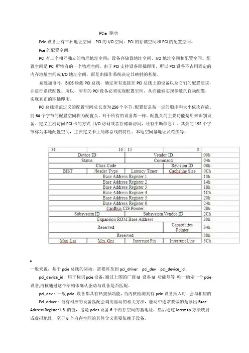
PCI总线规范定义的配置空间总长度为256个字节,配置信息按一定的顺序和大小依次存放。
前64个字节的配置空间称为配置头,对于所有的设备都一样,配置头的主要功能是用来识别设备、定义主机访问PCI卡的方式(I/O访问或者存储器访问,还有中断信息)。
其余的192个字节称为本地配置空间,主要定义卡上局部总线的特性、本地空间基地址及范围等。
•一般来说,基于pcie总线的驱动,需要涉及到pci_driver pci_dev pci_device_id .pci_device_id : 用于标识pcie设备,通过上图的厂商Id 设备Id 功能号等唯一确定一个pcie 设备,内核通过这个结构体确认驱动与设备是否匹配。
pci_dev : 一般pcie 设备都具有热拔插功能,当内核检测到有pcie设备插入时,会与相应的Pci_driver : 当有相应的设备匹配会调用驱动的相关方法,驱动中通常要做的是读出Base Adrress Register1-6 的值,这是pcies设备6个内存空间的基地址,然后通过ioremap方法映射成虚拟地址,至于6个内存空间的具体含义需要依赖于设备。
在用模块方式实现PCI设备驱动程序时,通常至少要实现以下几个部分:初始化设备模块、设备打开模块、数据读写和控制模块、中断处理模块、设备释放模块、设备卸载模块。
kernel用法-回复Kernel(核心)是计算机操作系统中的一个重要概念,它是操作系统的最基本组件,负责管理计算机的硬件资源和提供访问硬件的接口。
本文将以“kernel用法”为主题,介绍kernel的定义、功能、主要类型以及常用操作系统中kernel的应用。
一、kernel的定义和功能1. 定义:Kernel是操作系统的核心模块,是操作系统的一部分,负责管理计算机硬件资源和提供系统服务。
2. 功能:Kernel有以下几个主要功能:- 管理内存:Kernel负责对内存的分配、回收和管理,保证应用程序在内存中的运行。
- 管理进程:Kernel负责对进程的创建、调度和终止,保证多个进程之间的资源共享和协同工作。
- 管理文件系统:Kernel提供对文件系统的访问接口,包括文件的读写、创建、删除等操作。
- 设备驱动程序:Kernel负责管理和控制计算机硬件设备的驱动程序,使其可以与操作系统进行通信和交互。
- 网络功能:一些操作系统的kernel还提供网络功能,包括网络协议的支持、数据传输等。
二、kernel的主要类型1. 微内核(Microkernel):微内核是一种精简的kernel设计模式,只包含最核心的功能,其他功能通过服务程序(Server)来实现。
微内核的设计理念是将操作系统的复杂功能模块化,将不同的功能分离开来,以提高操作系统的可靠性和可扩展性。
2. 宏内核(Monolithic kernel):宏内核是一种将全部功能都集成到一个kernel中的设计模式。
宏内核包含了操作系统的所有功能,如内存管理、进程管理、文件系统等,所有功能通过一个统一的内核进行管理和调度。
宏内核的设计理念是将操作系统的功能紧密集成在一起,以提高操作系统的性能和响应速度。
3. 混合内核(Hybrid kernel):混合内核是微内核和宏内核的结合体,将一部分功能设计成微内核的形式,而其他功能则设计成宏内核的形式。
混合内核的设计理念是在宏内核的基础上,通过抽象和模块化的方式提高操作系统的可靠性和可扩展性。
MCU休眠唤醒原理详解1. 引言MCU(Microcontroller Unit,微控制器单元)是一种集成了处理器核心、存储器、外设接口和其他辅助电路的单芯片微型计算机。
在许多嵌入式系统中,为了节省能量和延长电池寿命,MCU通常会进入休眠状态。
当需要执行某些任务时,MCU通过唤醒机制被重新激活。
本文将详细介绍MCU休眠唤醒的基本原理,包括不同类型的休眠模式、唤醒源、唤醒过程和实现方法等。
2. MCU休眠模式MCU可以进入不同的休眠模式以降低功耗。
常见的几种休眠模式如下:2.1. 停止模式(Stop Mode)在停止模式下,MCU停止执行指令,并关闭大部分外设电源。
只有少数必要的外设(如RTC)保持运行。
停止模式是最低功耗的休眠模式,但需要较长时间来恢复。
2.2. 待机模式(Standby Mode)待机模式下,MCU停止执行指令,并关闭所有外设电源。
唯一保持运行的是待机唤醒电源和RTC。
待机模式的功耗较低,但恢复时间比停止模式快。
2.3. 休眠模式(Sleep Mode)休眠模式下,MCU停止执行指令,并关闭大部分外设电源。
但一些关键外设(如定时器和UART)可能会保持运行。
休眠模式的功耗较低,且恢复时间相对较快。
2.4. 睡眠模式(Sleep Mode)睡眠模式下,MCU停止执行指令,并关闭大部分外设电源。
只有少数关键外设(如中断控制器)保持运行。
睡眠模式的功耗较低,且恢复时间较短。
3. 唤醒源在MCU休眠状态下,需要一个或多个唤醒源来触发唤醒操作。
常见的唤醒源包括:3.1. 外部中断外部中断是通过引脚连接到MCU的外部信号触发的。
当引脚上出现特定的电平变化时,MCU就会被唤醒。
3.2. 内部中断内部中断是由MCU内部产生的信号触发的。
例如,定时器溢出中断可以设置为唤醒源,当定时器计数达到设定值时,MCU就会被唤醒。
3.3. 看门狗定时器看门狗定时器是一种特殊的定时器,用于监控系统的运行状态。
AVR单片机进入睡眠状态及唤醒的C语言程序M16掉电模式的耗电情况(看门狗关闭),时钟为内部RC 1MHz0.9uA@Vcc=5.0V [手册的图表约为1.1uA]0.3uA@Vcc=3.3V [手册的图表约为0.4uA]//测量的数字万用表是FLUKE 15B,分辨率0.1uA这个程序需要MCU进入休眠状态,为实现最低功耗,JTAG接口会被关闭,只能通过LED的变化来观察程序的运行。
这个实验里面,用STK500(AVRISP) ISP下载线来烧录更方便。
熔丝位设置1 关断BOD功能 BODEN=12 如果用ISP方式烧录,就可以完全关闭JTAG口了 OCEEN=1,JTAGEN=1*/#include <avr/io.h>#include <avr/signal.h>#include <avr/interrupt.h>#include <avr/delay.h>//时钟定为内部RC 1MHz,F_CPU=1000000 也可以采用其他时钟#include <avr/sleep.h>/*sleep.h里面定义的常数,对应各种睡眠模式#define SLEEP_MODE_IDLE 0空闲模式#define SLEEP_MODE_ADC _BV(SM0)ADC 噪声抑制模式#define SLEEP_MODE_PWR_DOWN _BV(SM1)掉电模式#define SLEEP_MODE_PWR_SAVE (_BV(SM0) | _BV(SM1))省电模式#define SLEEP_MODE_STANDBY (_BV(SM1) | _BV(SM2))Standby 模式#define SLEEP_MODE_EXT_STANDBY (_BV(SM0) | _BV(SM1) | _BV(SM2)) 扩展Standby模式函数void set_sleep_mode (uint8_t mode);设定睡眠模式void sleep_mode (void);进入睡眠状态*///管脚定义#define LED 0 //PB0 驱动LED,低电平有效#define KEY_INT2 0 //PB3 按键,低电平有效void delay_10ms(unsigned int t){/*由于内部函数_delay_ms() 最高延时较短262.144mS@1MHz / 32.768ms@8MHz / 16.384ms@16MHz故编写了这条函数,实现更长的延时,并能令程序能适应各种时钟频率*/while(t--)_delay_ms(10);}int main(void){unsigned char i;//上电默认DDRx=0x00,PORTx=0x00 输入,无上拉电阻PORTA=0xFF; //不用的管脚使能内部上拉电阻。
linux驱动程序之电源管理之标准linux休眠与唤醒机制分析(⼀)linux驱动程序之电源管理之标准linux休眠与唤醒机制分析(⼀)1. Based on linux2.6.32, only for mem(SDR)2. 有兴趣请先参考阅读:电源管理⽅案APM和ACPI⽐较.docLinux系统的休眠与唤醒简介.doc3. 本⽂先研究标准linux的休眠与唤醒,android对这部分的增改在另⼀篇⽂章中讨论4. 基于⼿上的⼀个项⽬来讨论,这⾥只讨论共性的地⽅虽然linux⽀持三种省电模式:standby、suspend to ram、suspend to disk,但是在使⽤电池供电的⼿持设备上,⼏乎所有的⽅案都只⽀持STR模式(也有同时⽀持standby模式的),因为STD模式需要有交换分区的⽀持,但是像⼿机类的嵌⼊式设备,他们普遍使⽤nand来存储数据和代码,⽽且其上使⽤的⽂件系统yaffs⼀般都没有划分交换分区,所以⼿机类设备上的linux都没有⽀持STD省电模式。
⼀、项⽬power相关的配置⽬前我⼿上的项⽬的linux电源管理⽅案配置如下,.config⽂件的截图,当然也可以通过makemenuconfig使⽤图形化来配置:## CPU Power Management## CONFIG_CPU_IDLE is not set## Power management options#CONFIG_PM=y# CONFIG_PM_DEBUG is not setCONFIG_PM_SLEEP=yCONFIG_SUSPEND=yCONFIG_SUSPEND_FREEZER=yCONFIG_HAS_WAKELOCK=yCONFIG_HAS_EARLYSUSPEND=yCONFIG_WAKELOCK=yCONFIG_WAKELOCK_STAT=yCONFIG_USER_WAKELOCK=yCONFIG_EARLYSUSPEND=y# CONFIG_NO_USER_SPACE_SCREEN_ACCESS_CONTROL is not set# CONFIG_CONSOLE_EARLYSUSPEND is not setCONFIG_FB_EARLYSUSPEND=y# CONFIG_APM_EMULATION is not set# CONFIG_PM_RUNTIME is not setCONFIG_ARCH_SUSPEND_POSSIBLE=yCONFIG_NET=y上⾯的配置对应下图中的下半部分图形化配置。
pcie设备休眠唤醒调用函数
在PCIE设备的驱动中,休眠和唤醒是必不可少的操作。
休眠可以节省设备的能量,而唤醒则可以恢复设备的正常工作。
为了实现PCIE设备的休眠唤醒功能,需要在驱动中调用相应的函数。
在Linux驱动中,常用的休眠唤醒函数有两种:
1. pm_runtime_suspend和pm_runtime_resume
这两个函数是Power Management Runtime框架中提供的,用于控制设备的电源状态。
pm_runtime_suspend函数可以让设备进入休眠状态,pm_runtime_resume函数则可以让设备从休眠状态中恢复。
2. pci_save_state和pci_restore_state
这两个函数是PCI总线驱动中提供的,用于保存和恢复设备的状态。
pci_save_state函数可以将设备的寄存器状态保存到内存中,pci_restore_state函数则可以将内存中保存的状态恢复到设备中。
在调用这些函数之前,需要先进行一些准备工作,如获取设备的句柄、初始化设备等。
具体的调用方法可以参考相应的API文档。
总之,在PCIE设备的驱动中,休眠唤醒是非常重要的功能,需要仔细调用相应的函数,确保设备能够正常运行。
- 1 -。
Rockchip休眠唤醒开发指南发布版本:0.1日期:2016.07前言概述产品版本读者对象本文档(本指南)主要适用于以下工程师:技术支持工程师软件开发工程师修订记录目录1休眠唤醒 .................................................................................................... 1-11.1概述.................................................................................................. 1-11.2重要概念............................................................................................. 1-11.3功能特点............................................................................................. 1-11.4开发指引............................................................................................. 1-1Rockchip休眠唤醒开发指南1休眠唤醒1休眠唤醒1.1概述1.现在芯片级的休眠唤醒操作主要在ATF中,这部分代码是没有开放的,为满足不同的产品需求,可以通过DTS配置系统SLEEP时进入不同的低功耗模式。
2.不同的项目对唤醒源的需求不同,在DTS中可以配置对应的唤醒源使能。
3.RK3399有4路PWM,不同的硬件上可能有用到若干路作为调压使用,为保证稳定性需要再休眠之前必须设置PWM控制的几路电压为默认电压,唤醒恢复。
内核睡眠函数1. 什么是内核睡眠函数内核睡眠函数是指在Linux内核中,用于使整个系统休眠的函数。
在Linux中,休眠是非常重要的一种操作,因为它可以在没有任务需要处理时,让系统进入一个低功耗模式,从而节省系统资源,减少对环境的影响。
2. 内核睡眠函数的分类内核睡眠函数一般分为两类:非阻塞式睡眠函数和阻塞式睡眠函数。
非阻塞式睡眠函数主要包括:timer_nanosleep()、do_nanosleep()、schedule_timeout()等。
这些函数的作用是休眠一段时间后,再重新运行程序。
这种睡眠方式并不会阻塞其他程序的运行,因此比较适合应用在实时性要求比较高的场合。
阻塞式睡眠函数主要包括:等待队列和信号量等。
这些函数会使当前进程进入睡眠状态,直到某个事件发生才会返回。
这种睡眠方式比较适合应用在非实时环境下,因为它可能会阻塞其他进程的运行。
3. 内核睡眠函数的实现原理内核睡眠函数的实现原理与CPU的休眠模式有关。
在CPU空闲时,内核会将CPU的各个寄存器状态保存到内存中,并从内存中读取一个保存在硬件中的休眠状态。
此时,CPU的时钟频率将降低,从而减少功耗,同时系统的其余部分也将降低功耗。
当需要唤醒CPU时,内核会将CPU的状态从内存中恢复出来,并重新启动CPU。
4. 内核睡眠函数的应用内核睡眠函数在Linux内核中广泛应用于各种场合,其中最常见的应用场合是:设备休眠、进程间同步等。
设备休眠是指将一个设备进行休眠,以节省能源。
设备在工作的时候,必然会占用一定的资源,而这些资源又很难被其他设备所共享,因此可以考虑将设备进行休眠。
设备休眠可以通过调用内核提供的休眠函数来实现。
进程间同步主要包括等待队列和信号量。
当多个进程共享某个资源时,很容易产生竞争条件,从而引发各种异常情况。
为了避免这种情况的发生,可以使用等待队列和信号量来进行同步。
这种处理方式也可以使用内核提供的休眠函数实现。
5. 总结内核睡眠函数在Linux内核中发挥着非常重要的作用。
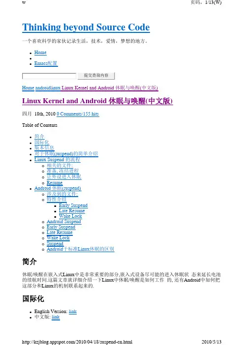
Linux Kernel and Android 休眠与唤醒(中文版) (转)简介休眠/唤醒在嵌入式Linux中是非常重要的部分,嵌入式设备尽可能的进入休眠状态来延长电池的续航时间.这篇文章就详细介绍一下Linux中休眠/唤醒是如何工作的, 还有Android中如何把这部分和Linux的机制联系起来的.版本信息∙Linux Kernel: v2.6.28∙Android: v2.0对于休眠(suspend)的简单介绍在Linux中,休眠主要分三个主要的步骤:1.冻结用户态进程和内核态任务2.调用注册的设备的suspend的回调函数o顺序是按照注册顺序3.休眠核心设备和使CPU进入休眠态冻结进程是内核把进程列表中所有的进程的状态都设置为停止,并且保存下所有进程的上下文. 当这些进程被解冻的时候,他们是不知道自己被冻结过的,只是简单的继续执行.如何让Linux进入休眠呢?用户可以通过读写sys文件/sys /power/state 是实现控制系统进入休眠. 比如命令系统进入休眠. 也可以使用来得到内核支持哪几种休眠方式.Linux Suspend 的流程相关的文件:你可以通过访问Linux内核网站来得到源代码,下面是文件的路径: ∙linux_soruce/kernel/power/main.c∙linux_source/kernel/arch/xxx/mach-xxx/pm.c∙linux_source/driver/base/power/main.c接下来让我们详细的看一下Linux是怎么休眠/唤醒的. Let 's going to see how these happens.用户对于/sys/power/state 的读写会调用到 main.c中的state_store(), 用户可以写入 const char * const pm_state[] 中定义的字符串, 比如"mem", "standby".然后state_store()会调用enter_state(), 它首先会检查一些状态参数,然后同步文件系统. 下面是代码:准备, 冻结进程当进入到suspend_prepare()中以后, 它会给suspend分配一个虚拟终端来输出信息, 然后广播一个系统要进入suspend的Notify, 关闭掉用户态的helper 进程, 然后一次调用suspend_freeze_processes()冻结所有的进程, 这里会保存所有进程当前的状态, 也许有一些进程会拒绝进入冻结状态, 当有这样的进程存在的时候, 会导致冻结失败,此函数就会放弃冻结进程,并且解冻刚才冻结的所有进程.让外设进入休眠现在, 所有的进程(也包括workqueue/kthread) 都已经停止了, 内核态人物有可能在停止的时候握有一些信号量, 所以如果这时候在外设里面去解锁这个信号量有可能会发生死锁, 所以在外设的suspend()函数里面作lock/unlock 锁要非常小心,这里建议设计的时候就不要在suspend()里面等待锁. 而且因为suspend的时候,有一些Log是无法输出的,所以一旦出现问题,非常难调试.然后kernel在这里会尝试释放一些内存.最后会调用suspend_devices_and_enter()来把所有的外设休眠, 在这个函数中, 如果平台注册了suspend_pos(通常是在板级定义中定义和注册), 这里就会调用 suspend_ops->begin(), 然后driver/base/power/main.c 中的device_suspend()->dpm_suspend() 会被调用,他们会依次调用驱动的suspend() 回调来休眠掉所有的设备.当所有的设备休眠以后, suspend_ops->prepare()会被调用, 这个函数通常会作一些准备工作来让板机进入休眠. 接下来Linux,在多核的CPU中的非启动CPU会被关掉, 通过注释看到是避免这些其他的CPU造成race condion,接下来的以后只有一个CPU在运行了.suspend_ops 是板级的电源管理操作, 通常注册在文件arch/xxx/mach-xxx/pm.c 中.接下来, suspend_enter()会被调用, 这个函数会关闭arch irq, 调用device_power_down(), 它会调用suspend_late()函数, 这个函数是系统真正进入休眠最后调用的函数, 通常会在这个函数中作最后的检查. 如果检查没问题, 接下来休眠所有的系统设备和总线, 并且调用 suspend_pos->enter() 来使CPU进入省电状态. 这时候,就已经休眠了.代码的执行也就停在这里了.Resume如果在休眠中系统被中断或者其他事件唤醒, 接下来的代码就会开始执行, 这个唤醒的顺序是和休眠的循序相反的,所以系统设备和总线会首先唤醒,使能系统中断, 使能休眠时候停止掉的非启动CPU, 以及调用suspend_ops->finish(), 而且在suspend_devices_and_enter()函数中也会继续唤醒每个设备,使能虚拟终端, 最后调用 suspend_ops->end().在返回到enter_state()函数中的, 当 suspend_devices_and_enter() 返回以后, 外设已经唤醒了, 但是进程和任务都还是冻结状态, 这里会调用suspend_finish()来解冻这些进程和任务, 而且发出Notify来表示系统已经从suspend状态退出, 唤醒终端.到这里, 所有的休眠和唤醒就已经完毕了, 系统继续运行了.Android 休眠(suspend)在一个打过android补丁的内核中, state_store()函数会走另外一条路,会进入到request_suspend_state()中, 这个文件在earlysuspend.c中. 这些功能都是android系统加的, 后面会对earlysuspend和late resume 进行介绍.涉及到的文件:∙linux_source/kernel/power/main.c∙linux_source/kernel/power/earlysuspend.c∙linux_source/kernel/power/wakelock.c特性介绍Early SuspendEarly suspend 是android 引进的一种机制, 这种机制在上游备受争议,这里不做评论. 这个机制作用在关闭显示的时候, 在这个时候, 一些和显示有关的设备, 比如LCD背光, 比如重力感应器, 触摸屏, 这些设备都会关掉, 但是系统可能还是在运行状态(这时候还有wake lock)进行任务的处理, 例如在扫描SD卡上的文件等. 在嵌入式设备中, 背光是一个很大的电源消耗,所以android会加入这样一种机制.Late ResumeLate Resume 是和suspend 配套的一种机制, 是在内核唤醒完毕开始执行的. 主要就是唤醒在Early Suspend的时候休眠的设备.Wake LockWake Lock 在Android的电源管理系统中扮演一个核心的角色. Wake Lock是一种锁的机制, 只要有人拿着这个锁, 系统就无法进入休眠, 可以被用户态程序和内核获得. 这个锁可以是有超时的或者是没有超时的, 超时的锁会在时间过去以后自动解锁. 如果没有锁了或者超时了, 内核就会启动休眠的那套机制来进入休眠.Android Suspend当用户写入mem 或者 standby到 /sys/power/state中的时候, state_store()会被调用, 然后Android会在这里调用 request_suspend_state() 而标准的Linux会在这里进入enter_state()这个函数. 如果请求的是休眠, 那么early_suspend这个workqueue就会被调用,并且进入early_suspend状态.Early Suspend在early_suspend()函数中, 首先会检查现在请求的状态还是否是suspend, 来防止suspend的请求会在这个时候取消掉(因为这个时候用户进程还在运行),如果需要退出, 就简单的退出了. 如果没有, 这个函数就会把early suspend中注册的一系列的回调都调用一次, 然后同步文件系统, 然后放弃掉main_wake_lock, 这个wake lock是一个没有超时的锁,如果这个锁不释放, 那么系统就无法进入休眠.Late Resume当所有的唤醒已经结束以后, 用户进程都已经开始运行了, 唤醒通常会是以下的几种原因:∙来电如果是来电, 那么Modem会通过发送命令给rild来让rild通知WindowManager 有来电响应,这样就会远程调用PowerManagerService来写"on" 到/sys/power/state 来执行late resume的设备, 比如点亮屏幕等.∙用户按键用户按键事件会送到WindowManager中, WindowManager会处理这些按键事件,按键分为几种情况, 如果案件不是唤醒键(能够唤醒系统的按键) 那么WindowManager会主动放弃wakeLock来使系统进入再次休眠, 如果按键是唤醒键,那么WindowManger就会调用PowerManagerService中的接口来执行 Late Resume.∙Late Resume 会依次唤醒前面调用了Early Suspend的设备.Wake Lock我们接下来看一看wake lock的机制是怎么运行和起作用的, 主要关注wakelock.c文件就可以了.wake lock 有加锁和解锁两种状态, 加锁的方式有两种, 一种是永久的锁住, 这样的锁除非显示的放开, 是不会解锁的, 所以这种锁的使用是非常小心的. 第二种是超时锁, 这种锁会锁定系统唤醒一段时间, 如果这个时间过去了, 这个锁会自动解除.锁有两种类型:1.WAKE_LOCK_SUSPEND 这种锁会防止系统进入睡眠2.WAKE_LOCK_IDLE 这种锁不会影响系统的休眠, 作用我不是很清楚.在wake lock中, 会有3个地方让系统直接开始suspend(), 分别是:1.在wake_unlock()中, 如果发现解锁以后没有任何其他的wake lock了,就开始休眠2.在定时器都到时间以后, 定时器的回调函数会查看是否有其他的wakelock, 如果没有, 就在这里让系统进入睡眠.3.在wake_lock() 中, 对一个wake lock加锁以后, 会再次检查一下有没有锁, 我想这里的检查是没有必要的, 更好的方法是使加锁的这个操作原子化, 而不是繁冗的检查. 而且这样的检查也有可能漏掉. Suspend当wake_lock 运行 suspend()以后, 在wakelock.c的suspend()函数会被调用,这个函数首先sync文件系统,然后调用pm_suspend(request_suspend_state),接下来pm_suspend()就会调用enter_state()来进入Linux的休眠流程..Android于标准Linux休眠的区别pm_suspend() 虽然会调用enter_state()来进入标准的Linux休眠流程,但是还是有一些区别:∙当进入冻结进程的时候, android首先会检查有没有wake lock,如果没有, 才会停止这些进程, 因为在开始suspend和冻结进程期间有可能有人申请了 wake lock,如果是这样, 冻结进程会被中断.∙在 suspend_late()中, 会最后检查一次有没有wake lock, 这有可能是某种快速申请wake lock,并且快速释放这个锁的进程导致的,如果有这种情况, 这里会返回错误, 整个suspend就会全部放弃.如果pm_suspend()成功了,LOG的输出可以通过在kernel cmd里面增加"no_console_suspend" 来看到suspend和resume过程中的log输出。