Poisson Image Editing

泊松融合matlab
泊松融合是一种常用的图像处理算法，可以将两张不同的图片合并成一张完整的图片。

这种算法在数码相机、电影特效以及计算机视觉领域都有很广泛的应用。

在matlab中，实现泊松融合可以使用Image Processing Toolbox中的函数。

泊松融合的基本思路是将两张图像进行“剪切”和“粘贴”操作，即将一张图像中的某些区域剪切出来，然后将其粘贴到另一张图像中。

为了使得两张图像的边缘能够自然地衔接，需要使用泊松方程进行修正，从而达到更好的融合效果。

在matlab中，可以使用如下代码实现泊松融合：
```matlab
% 读入两张图像
A = imread('image1.jpg');
B = imread('image2.jpg');
% 获取A图像中需要剪切的区域
mask = roipoly(A);
% 对A图像中的剪切区域进行泊松融合
blended_image = poissonBlend(B, A, mask);
% 显示融合后的图像
imshow(blended_image);
```
上述代码中，通过调用roipoly函数获取图像A中需要剪切的区
域，然后使用poissonBlend函数进行泊松融合操作，最终得到融合后的图像。

需要注意的是，将两张图像进行泊松融合时，需要保证两张图像的大小和分辨率相同。

除了使用matlab自带的函数实现泊松融合之外，还可以使用第三方工具包，如OpenCV、Python等进行实现。

无论使用哪种工具包，都需要对泊松融合的算法原理有一定的了解，才能够更好地实现该算法。

泊松融合原理和python代码泊松融合（Poisson blending）是一种图像处理技术，用于将源图像中的对象融合到目标图像中，以实现无缝的图像合成。

该技术通过泊松方程求解，在图像融合中起到关键作用。

泊松融合的基本原理是通过将源图像中的像素值通过泊松方程融合到目标图像中，从而在目标图像中生成一个新的像素值，以实现图像融合的效果。

其数学表示如下：∇²α=∂²α/∂x²+∂²α/∂y²=β其中，α表示源图像中的像素值，β表示目标图像中的边缘像素值。

这个方程可以简化为拉普拉斯方程∆α=β，其中∆表示拉普拉斯算子。

这个方程的意义是，对于源图像中的像素α，其梯度的变化应该与目标图像中的边缘像素β相匹配。

根据泊松方程求解的目标，可以得到融合后的像素值。

在求解过程中，需要考虑边界条件和约束条件。

边界条件通常是指融合图像的边界像素值应与目标图像一致，约束条件通常是指源图像中的一些区域或者像素需要完全复制到目标图像中，从而实现融合效果。

下面是一个使用Python实现泊松融合的代码示例：```pythonimport numpy as npfrom scipy.sparse import linalgdef poisson_blend(source, target, mask):#获取图像的宽度和高度height, width, _ = target.shape#创建拉普拉斯矩阵A和边界像素矩阵bA = np.zeros((height * width, height * width))b = np.zeros(height * width)#根据源图像和目标图像计算拉普拉斯矩阵A和边界像素矩阵bfor y in range(1, height - 1):for x in range(1, width - 1):#当前像素在图像中的索引idx = y * width + xif mask[y, x] == 1:#如果是掩膜内的像素，使用泊松方程并加上约束条件A[idx, idx] = 4A[idx, idx - 1] = -1A[idx, idx + 1] = -1A[idx, idx - width] = -1A[idx, idx + width] = -1b[idx] = 4 * source[y, x] - source[y, x - 1] - source[y, x + 1] - source[y - 1, x] - source[y + 1, x]else:#如果是边界像素，直接复制到目标图像中A[idx, idx] = 1b[idx] = target[y, x]#使用稀疏矩阵求解线性方程组x = linalg.spsolve(A, b)# 将求解出的像素值reshape为目标图像的形状blend = x.reshape((height, width, 3)) return blend#加载源图像、目标图像和掩膜图像source = np.array(Image.open('source.jpg')) target = np.array(Image.open('target.jpg')) mask = np.array(Image.open('mask.png'))#对源图像和目标图像进行泊松融合blend = poisson_blend(source, target, mask) #显示融合后的图像plt.imshow(blend)plt.show```这段代码使用了`numpy`库和`scipy.sparse`库实现了泊松融合的算法。

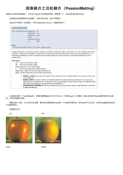
图像融合之泊松融合（PossionMatting）前⾯有介绍拉普拉斯融合，今天说下OpenCV泊松融合使⽤。

顺便提⼀下，泊松是拉普拉斯的学⽣。

泊松融合的原理请参考这篇博⽂，讲的⾮常详细，此处不再赘述。

OpenCV中集成了泊松融合，API为seamless Clone()，函数原型如下： 泊松融合是将⼀个src放进dst中，放置位置根据dst中P点为中⼼的⼀个前景mask⼤⼩范围内。

融合过程会改变src图像中颜⾊以及梯度，达到⽆缝融合效果。

需要注意⼀点是，中⼼点P点的设置，最好是先根据前景mask算⼀个外接矩形框Rect，取Rect的中⼼点为P，保证Rect能够放进dst中，不会越界就好。

效果展⽰如下： src dstmask blend⽰例代码：1 #include <opencv2\opencv.hpp>2 #include <iostream>3 #include <string>45using namespace std;6using namespace cv;789void main()10 {11 Mat imgL = imread("data/apple.jpg");12 Mat imgR = imread("data/orange.jpg");1314int imgH = imgR.rows;15int imgW = imgR.cols;16 Mat mask = Mat::zeros(imgL.size(), CV_8UC1);17 mask(Rect(0,0, imgW*0.5, imgH)).setTo(255);18 cv::imshow("mask", mask);19 Point center(imgW*0.25, imgH*0.5);2021 Mat blendImg;22 seamlessClone(imgL, imgR, mask, center, blendImg, NORMAL_CLONE); 2324 cv::imshow("blendimg", blendImg);25 waitKey(0);26 }。

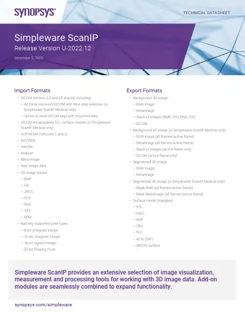
Import Formats• DICOM (version 3.0 and 2D stacks) including:–4D (time-resolved) DICOM with time step selection (in Simpleware ScanIP Medical only)–Option to store DICOM tags with imported data • DICOM encapsulated STL surface models (in Simpleware ScanIP Medical only)• ACR-NEMA (versions 1 and 2)• DICONDE • Interfile • Analyze • Meta-image • Raw image data • 2D image stacks: –BMP –GIF –JPEG –PCX –PNG –TIFF –XPM• Natively supported pixel types: –8-bit Unsigned Integer –16-bit Unsigned Integer –16-bit Signed Integer –32-bit Floating PointTECHNICAL DATASHEETExport Formats• Background 3D image: –RAW image –MetaImage–Stack of images (BMP , JPG, PNG, TIF) –DICOM• Background 4D image (in Simpleware ScanIP Medical only): –RAW image (all frames/active frame) –MetaImage (all frames/active frame) –Stack of images (active frame only) –DICOM (active frame only)• Segmented 3D image: –RAW image –MetaImage• Segmented 4D image (in Simpleware ScanIP Medical only): –Mask RAW (all frames/active frame) –Mask MetaImage (all frames/active frame)• Surface model (triangles): –STL –IGES –3MF –OBJ –PLY –ACIS (SAT) –ANSYS surfaceSimpleware ScanIP provides an extensive selection of image visualization, measurement and processing tools for working with 3D image data. Add-on modules are seamlessly combined to expand functionality.Simpleware ScanIPRelease Version U-2022.12Export Formats cont.• Surface model (triangles) cont.:–ABAQUS surface–OPEN INVENTOR–POINT CLOUD–MATLAB file surface–DICOM encapsulated STL (in SimplewareScanIP Medical only)• Animations:–AVI–Ogg Theora–H.264/MPEG-4 AVC–Windows Media Video (WMV)–PNG sequence–Transparent PNG sequence• 2D and 3D screenshot:–JPEG–PNG–Postscript (*.eps)–BMP–PNM–PDF• Generate virtual X-Ray, with object burn (in SimplewareScanIP Medical only)• Export scene – export the current 3D view:–3D PDF–3MF–OBJ–PLY–VRMLGeneral User Interface• Modern ribbon interface• Custom ribbon with user-selected tools (My tools)• Quick find search feature for tools• User-defined customization: dockable toolboxes, range of2D/3D view options• Undo/redo operation support• Independent part visibility control in 2D and 3D• Keyboard shortcuts: set user-defined shortcuts to commands or tools to customize and speed up repeated workflows• Ability to import multiple image sets into the workspace toaid segmentation• Histogram and profile line utilities assist in finding optimalthreshold values• Automatic logging and timestamp of filters and tools applied since the creation of a project• Workspace tabs: toggle between the active document, mask statistics, model statistics, centerline statistics, the document log, and the scripting interface• Integrated dynamic help tool• Interactive tutorials• Links to external support resources• Preferences: a number of different options available fordefault settings:–General: number of undos to save, default startup layout,max permissible CPUs for parallelized operations–Slice views: display orientation labels, choose whether touse a dark background, specify model contour and maskvoxel outline colors–PACS (in Simpleware ScanIP Medical only): two-way PACScommunication, configure access (servers, ports, keys etc.)–Segmentation: options to adjust behavior of somesegmentation tools and set Hounsfield presets forthe Threshold tool–3D view: save last camera position before exiting thedocument, stereo rendering settings, options to furtherdivide higher-order mesh elements (for FE meshesand NURBS patches)–Volume rendering: GPU rendering supported, Backgroundvolume rendering visibility on startup–Folders: options to change locations of temporary files–Statistics: default template for Mask, Model andCenterline statistics–Number formatting: customize how numbers are formatted within Simpleware ScanIP–Annotations: set default styles for annotations–Scripting: enable/disable supported scripting languages–Licensing: change license location–Miscellaneous: reset suppressible dialogs, clear the undo/redo stack, mask name/color creation options2D User Interface• 3x 2D views• Orientation labels• Scale bars• DICOM information overlay (in SimplewareScanIP Medical only)• Interactive cropping using 2D view• Window/Level values and control options• Ability to work on single slice, selection of slicesor whole volume• Slice cursors to identify the position of 2D slices2D User Interface cont.• Mask visualization options: solid, translucent, voxel outline • View 3D model contours from model/3D view, surface objects and volume meshes on 2D slices• Multi-planar reconstruction through translation and rotation of reslicing axes3D User Interface• Background volume rendering: using standard presets orgreyscale mapping• Single mask volume rendering• Interactive cropping using 3D view• Clipping box: unconstrained, interactive sectioningof 3D rendering• Fast 3D preview mode for rapid visualization of segmentation: ability to change preview quality to speed up rendering andreduce memory consumption• Live 3D: automatic 3D volume rendering refresh of masks • Mask transparency• Wireframe mode• Vertex lines superimposed over surfaces mode• Lighting and 3D rendering adjustments• Background adjustments:–Single color–Two color gradient–Skybox• View surface entities: CFD boundary conditions, node sets,contacts, shells• View contours of greyscale-based material properties• Model shading options: None, flat, Gouraud, hardware shader • Fullscreen mode• Camera control tool• Load and save 3D view camera positions• View slice planes• Slice intersection position widget• Show image dimensions on scale axes• 3D stereoscopic visualization with selected hardwaremodes available:–Crystal eyes–Red/blue–Interlaced–Left–Right–Dresden–Anaglyph–Checkerboard Image Processing Tools• Data processing:–Crop–Pad–Rescale–Shrink wrap–Resample using various interpolation techniques: nearestneighbor, linear, majority wins and partial volume effects–Flip–Shear–Align–Register datasets: Align background images to otherbackground images or any other dataset type based onsets of landmark points and/or automatic greyscale-based registration• Basic filters (most commonly used):–Smoothing: Recursive Gaussian, Smart masksmoothing, De-stepping–Noise filtering: mean filter, median filter–Cavity fill–Island removal filter–Fill gaps tool (using largest contact surface or mask priority)• Advanced filters (more specialist applications):–Binarization–Combine backgrounds–Connected component–Gradient magnitude–Lattice factory–Local maxima–MRI bias field correction (N4)–Masking filter–Morphological by reconstruction–Sigmoid–Simplify partial volume–Slice propagate–Distance maps:–Danielsson–Signed Maurer–CT correction:–CT image stabilizer–Histogram cylindrical equalization–Histogram slice equalization–Metal artefact reductionImage Processing Tools cont.• Advanced filters (more specialist applications) cont.:–Smoothing and noise removal:–Bilateral–Curvature anisotropic diffusion–Curvature flow–Discrete Gaussian–Gradient anisotropic diffusion–Min/max curvature flow–Patch-based denoising–Level sets:–Canny segmentation–Fast marching–Geodesic active contours–Laplacian level set–Shape detection–Threshold level set–Skeletonization:–Pruning–Thinning• Morphological filters:–Erode–Dilate–Open–Close–3D Wrap• Segmentation tools:–Paint/unpaint–Paint with threshold–Smart paint–Interpolation toolbox – Contains the following options:–Slice interpolation: smooth or linear–Slice propagation: adapts to image or uses direct copy–Confidence connect region growing–Background flood fill–Mask flood fill–Threshold–3D editing tools for application of filters to local regions –option to apply in multiple regions and on camera facingsurface only in advanced tool version–Mask ungroup tool–Automated generation of masks for pre- segmented images –Magnetic lasso–Multilevel Otsu segmentation–Split regions tool, with the ability to markregions in the 3D view–Merge regions tool–Direct copy: background to mask or mask to background–Watershed segmentation tool• Boolean operations: applied to/between masks. General and Venn diagram UI options:–Union–Intersect–Subtract–Invert• Local surface correction: local, greyscale-informed correction of mask surface, including the ability to apply on a regionof interest only• Multi-label tools: use mask labels to label different regionswithin a mask. Use for statistics and visualization:–Label disconnected regions–Split mask into pores–Combine masks to multi-label mask–Mask label editor–Reports (automatically generate pre-formatted reportsof common metrics using a multi-label mask orfull model’s mesh):–Particles report–Pores and throats report• Window/level tool• Overlap check: display/generate mask to check overlapvolume in active masksStatistical Analysis• Quick statistics: quickly compute commonly requiredquantities (volume, surface area, average greyscale, etc.)• Mask statistics (based on voxel information):–Built-in templates: general statistics, contact statistics,material statistics, orientation, pore sizes, surface statistics –Ability to generate user-defined templates–Variety of statistical information pertaining to:–Voxels: count, volume, surface area, etc.–Greyscales: mean, standard deviation,minimum, maximum, etc.–Surface estimation: area, area fraction, volume,volume fraction, etc.–Material properties: mass, mass density, Young’s modulus,Poisson’s ratio, moment of inertia, etc.–Axis-aligned bounding boxes–Axis-aligned bounding ellipsoidsStatistical Analysis cont.• Mask statistics (based on voxel information) cont.:–Object-oriented bounding boxes–Object-oriented bounding ellipsoids–Create a user-defined statistic• Model statistics (based on polygon information):–Ability to generate user-defined templates–Built-in templates: general statistics (perimeters, surfaces,volumes and NURBS surfaces), mesh quality (CFD, FE-linear elements and FE-quadratic elements), orientation(perimeters, surfaces, volumes), pore sizes, surface quality(linear, quadratic), volume mesh statistics–Variety of statistical information pertaining to:–Surface parameters: element count, node count,edge count, etc.–Perimeters: length, mean edge length, meandihedral angle, etc.–Surface triangle and quadrilateral primitives: edge- length,in-out ratio, distortion, etc.–Tetrahedral, hexahedral, pyramid and prismatic volumeelement primitives: angular skew, volume skew, shapefactor, Jacobian, etc.–Axis-aligned bounding boxes–Axis-aligned bounding ellipsoids–Object-oriented bounding boxes–Object-oriented bounding ellipsoids–Create a user-defined statistic• Centerline statistics:–Built-in templates: line orientation, lines by network, lines by node, constriction, shape, twist, nodes by network.–Ability to generate user-defined templates–Variety of statistical information pertaining to:–Lines: count, network, length, Euclidean length, curvature,torsion, closed, looped, positions, orientation, connectioncount, cross-sectional area and perimeter, incircle radius,twist, control points, object-oriented bounding boxes,mean orientation vector, best–fit circle, inscribed radius, circumscribed radius,bounding ellipse radius–Nodes: name, mask, network, position, line count,connection count.–Create a user-defined statistic–Probe centerlines to get measurements at specific locations • Save and import user-defined templates and statistics• Compute statistics within user-defined regions ofinterest (ROIs)Fiber Orientation Analysis• Allows fiber orientation to be analyzed directly from the image data (without the need for segmentation)• Option to include a mask representing the fiber region for fiber volume and diameter information• Specify the fiber diameter and the sampling size to beanalyzed for the whole image or a region of interest• Copy the centerlines generated during the analysis to thecenterlines editor for further editing or analysis• Statistics for analyzed region or region of interest:–Analyzed volume, fiber volume, fiber density,principal orientation–Eigen analysis (major, medial, minor vectors and value)–Orientation tensor–Fiber length and cross-section information• Plot statistics, export as *.png or *.csv:–Angle to principal orientation histogram–Angle to image axis histogram–Orientation tensor components vs image axis–Fiber density vs image axis (requires segmentation)–Principal orientation hedgehog diagram–Length of whole fibers histogram–Diameter of all segments histogram (incircle/best fit circle)(requires segmentation)• Visualize vectors:–Orientation vectors, Eigen vectors, Eigenellipsoids in 3D view–Orientation vectors in 2D slices–Change color scheme, and glyph density/scale/width–Export as *.csv or *.txt files• Map to mesh:–Export (or assign using FE Module) fiber orientationinformation per mesh cell–Average orientation tensor, eigenvector and eigenvalue data calculated for each mesh cell–Export volume fraction information per mesh cell(requires segmentation)Particle Analysis• Allows particles (either isolated or touching) to be analyzed from a mask or multi-label mask• There are two types of pore analysis available, “Touching”,for particles that are in contact with each other, “Isolated” for particles that are separated from each other.• Statistics for analyzed region or region of interest:–Particle volume (Total, Mean, SD, Min, Max)–Particle area (Mean, SD, Min, Max)–Particle volume fraction–Particle equivalent volume sphere diameter(Mean, SD, Min, Max)–Particle bounding box extent (Mean, SD, Min, Max)–Particle ellipsoid diameter (Mean, SD, Min, Max)–Particle flatness–Particle elongation–Particle shape factor–Particle sphericity• Plot statistics, export as *.png or *.csv:–Volume histogram–Area histogram–Flatness histogram–Elongation histogram–Shape factor histogram–Sphericity histogram• Particle visualization:–Contact count–Voxel count–Surface area–Boundary contact area–Label contact area–Volume–Max greyscale–Mean greyscale–Major length–Flatness–Elongation–Shape factor–Sphericity–Orientation angle to x/y/z axis–Orientation to mean–Export as *.csv or *.txt files• Map to mesh:–Export (or assign using FE Module) particle volume fraction information per mesh cell Pore Analysis• Allows pores (either open or closed) to be analyzed from a mask or multi-label mask• There are two types of pore analysis available, “Open”, for connected pore networks, and “Closed” for pores that are separated from each other• Statistics for analyzed region or region of interest:–Total pores count–Total throat count volume–Volume fraction–Internal pore volume (Mean, SD, Min, Max)–Internal pore surface area (Mean, SD, Min, Max)–Pore equivalent volume sphere diameter(Mean, SD, Min, Max)–Pore Flatness (Mean, SD, Min, Max)• Statistics for analyzed region or region of interest cont.–Pore Elongation (Mean, SD, Min, Max)–Pore Shape factor (Mean, SD, Min, Max)–Pore Sphericity (Mean, SD, Min, Max)–Pore coordination number (Mean, SD, Min, Max)–Throat contact count–Throat contact area–Throat radius (Mean, SD, Min, Max)–Throat Flatness (Mean, SD, Min, Max)–Throat Elongation (Mean, SD, Min, Max)–Throat Eccentricity (Mean, SD, Min, Max)–Throat Shape factor (Mean, SD, Min, Max)• Plot statistics, export as *.png or *.csv:–Volume histogram–Area histogram–Flatness histogram–Elongation histogram–Shape factor histogram–Sphericity histogram• Particle visualization:–Contact count–Voxel count–Surface area–Boundary contact area–Label contact area–Volume–Max greyscale–Mean greyscale–Major lengthPore Analysis cont.• Particle visualization cont.:–Flatness–Elongation–Shape factor–Sphericity–Orientation angle to x/y/z axis–Orientation to mean–Export as *.csv or *.txt files• Map to mesh:–Export (or assign using FE Module) pore volume fractioninformation per mesh cellSurface Mesh Generation• Topology and volume preserving smoothing• Triangle smoothing• Decimation• Multipart surface creation• Surface element quality control (for volume meshing in third party software)• So-called ‘sub-pixel accuracy’ through the use of partialvolume effects dataSurface Mesh Quality Inspection Tool• Inspect surface triangles or clusters of triangles• Option to show mesh errors (e.g. surface holes, surfaceintersections) and warnings• Show distorted elements above a user-defined threshold • Display quality metric histograms• Zoom into the pathological element to inspect it more closely Measurement Tools• Create and save points, distances and angles in 2D/3D• Visualization options to display all at once or selected• Snap to 3D surface option• Profile line• Histogram• Export as comma-separated values• Centerline creation toolkit:–Centerline creation (general)–Centerline creation for fibers–Junction editing• 2D contour measurements:–Creation mode–Area–Total perimeter–In-circle diameter–Out-circle diameter–Trigone-Trigone (TT) distance–Septal to Lateral (SL) distance–Intercommissural (IC) distance–Posterior perimeter• Wall thickness analysis tool for masks or surface objects,using a raycasting or sphere fitting algorithm• Shape-based measurement tools:–Shape editor: Create, edit, visualize, exportand measure shapes–Shape fitting: Fit shapes to geometry–Shape-to-shape measurements: Obtain measurementsbetween shape objects• X-ray image import, with alignment and object registration (in Simpleware ScanIP Medical only)3D Printing Toolkit• Set of tools for editing, analyzing and visualizing surfacesbefore sending them to a 3D printer which includes:–Preparation tools:–Model preview–Mask to Surface–Emboss text–Hollow–Cut–Create Connectors (inc. manual and automatic options)–Pins and Sockets connectors–Analysis tool – Greyscale visualization–Inspection tools:–Color proofing–Check printability–E xport: a variety of file formats including:–3MF–STL–OBJ–PLY–3D PDF–VRML©2022 Synopsys, Inc. All rights reserved. Synopsys is a trademark of Synopsys, Inc. in the United States and other countries. A list of Synopsys trademarks is available at /copyright.html . All other names mentioned herein are trademarks or registered trademarks of their respective owners.Animations• Create and export animations in the 3D view • Built-in-quick animations: –Rotations –Slice reveals –Volume rendering• User-defined animations cues: –Background colors–Camera (orbits, follow path and key frame-based), –Clipping –Opacity –2D slice planes –Volume rendering • Export formats: –AVI –Ogg Theora –H.264/MPEG-4 AVC–Windows Media Video (WMV) –PNG sequence• Variety of export sizes: From 480p to 2160p (4K)4D Frame Toolbox (in Simpleware ScanIP Medical only)• Active frame slider to manually control frame displayed in the 2D slice views and 3D view• Cine mode for active slice view and 3D view • Compare frames – compare two 2D slice views to examine differences• Options to set the time between frames and delete unwanted framesScripting• The ScanIP Application Programming Interface (API) is an object-oriented programming library that allows access to most of the features of Simpleware ScanIP • Support for a variety of scripting languages: –Python 3 –C#–Python 2 (deprecated) –Iron python (deprecated) –Visual basic (deprecated) –Boo (deprecated) –Java (deprecated)• Macro recording: record, save and play macro • Convert log entry to script• Script editor with autocomplete functionality• Console ScanIP: a GUI-less version of Simpleware ScanIP which can be run with scripted workflows。

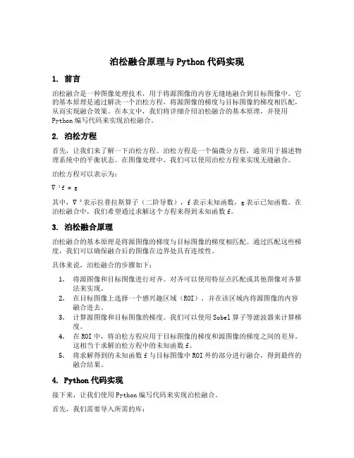
泊松融合原理与Python代码实现1. 前言泊松融合是一种图像处理技术，用于将源图像的内容无缝地融合到目标图像中。

它的基本原理是通过解决一个泊松方程，将源图像的梯度与目标图像的梯度相匹配，从而实现融合效果。

在本文中，我们将详细介绍泊松融合的基本原理，并使用Python编写代码来实现泊松融合。

2. 泊松方程首先，让我们来了解一下泊松方程。

泊松方程是一个偏微分方程，通常用于描述物理系统中的平衡状态。

在图像处理中，我们可以使用泊松方程来实现无缝融合。

泊松方程可以表示为：∇²f = g其中，∇²表示拉普拉斯算子（二阶导数），f表示未知函数，g表示已知函数。

在泊松融合中，我们希望通过求解这个方程来得到未知函数f。

3. 泊松融合原理泊松融合的基本原理是将源图像的梯度与目标图像的梯度相匹配。

通过匹配这些梯度，我们可以确保融合后的图像在边界处具有连续性。

具体来说，泊松融合的步骤如下：1.将源图像和目标图像进行对齐。

对齐可以使用特征点匹配或其他图像对齐算法来实现。

2.在目标图像上选择一个感兴趣区域（ROI），并在该区域内将源图像的内容融合进去。

3.计算源图像和目标图像的梯度。

我们可以使用Sobel算子等滤波器来计算梯度。

4.在ROI中，将泊松方程应用于目标图像的梯度和源图像的梯度之间的差异。

这相当于求解泊松方程中的未知函数f。

5.将求解得到的未知函数f与目标图像中ROI外的部分进行融合，得到最终的融合结果。

4. Python代码实现接下来，让我们使用Python编写代码来实现泊松融合。

首先，我们需要导入所需的库：import numpy as npimport cv2from scipy import sparsefrom scipy.sparse.linalg import spsolve然后，我们定义一个名为poisson_blend的函数来执行泊松融合：def poisson_blend(source, target, mask):# 获取源图像和目标图像的尺寸height, width, _ = source.shape# 将源图像和目标图像转换为灰度图像source_gray = cv2.cvtColor(source, cv2.COLOR_BGR2GRAY)target_gray = cv2.cvtColor(target, cv2.COLOR_BGR2GRAY)# 计算源图像和目标图像的梯度source_grad_x = cv2.Sobel(source_gray, cv2.CV_64F, 1, 0, ksize=3)source_grad_y = cv2.Sobel(source_gray, cv2.CV_64F, 0, 1, ksize=3)target_grad_x = cv2.Sobel(target_gray, cv2.CV_64F, 1, 0, ksize=3)target_grad_y = cv2.Sobel(target_gray, cv2.CV_64F, 0, 1, ksize=3)# 创建稀疏矩阵A和向量bA = sparse.lil_matrix((height * width, height * width))b = np.zeros((height * width,))# 填充矩阵A和向量bfor y in range(1,height-1):for x in range(1,width-1):if mask[y,x] == 255:index = y * width + xA[index,index] = -4A[index,index-1] = 1A[index,index+1] = 1A[index,index-width] = 1A[index,index+width] = 1b[index] = target_grad_x[y,x] - target_grad_x[y,x-1] + target_ grad_y[y,x] - target_grad_y[y-1,x]# 解泊松方程f = spsolve(A.tocsr(), b)# 将求解得到的未知函数f转换为图像f_image = np.uint8(np.clip(f.reshape(height, width), 0, 255))# 在目标图像中将ROI外的部分与源图像进行融合blended = target.copy()for y in range(height):for x in range(width):if mask[y,x] == 255:blended[y,x] = source[y,x]return blended最后，我们加载源图像、目标图像和蒙版，并调用poisson_blend函数来执行泊松融合：source = cv2.imread('source.jpg')target = cv2.imread('target.jpg')mask = cv2.imread('mask.jpg', cv2.IMREAD_GRAYSCALE)result = poisson_blend(source, target, mask)cv2.imwrite('result.jpg', result)5. 总结在本文中，我们详细介绍了泊松融合的基本原理，并使用Python编写了相应的代码实现。

泊松融合原理和python代码泊松融合是一种图像处理技术，可以将两幅图像进行平滑过渡，使其看起来自然无缝地融合在一起。

本文将介绍泊松融合的原理，并给出使用Python实现泊松融合的代码示例。

1. 泊松融合的原理2. 泊松融合的步骤3. 使用Python实现泊松融合的代码示例【1. 泊松融合的原理】泊松融合的原理是基于在两幅图像之间进行局部亮度和颜色平滑的假设。

具体来说，泊松融合可以看作是将源图像的颜色和边缘信息与目标图像的结构进行融合的过程。

【2. 泊松融合的步骤】泊松融合一般包括以下几个步骤：1) 输入源图像和目标图像。

2) 确定源图像在目标图像中的位置，以及需要融合的区域。

3) 对源图像和目标图像进行预处理，包括调整图像大小、灰度化等。

4) 使用梯度域重建技术计算源图像的梯度场。

5) 根据源图像的梯度向量和目标图像的结构特征进行优化，生成泊松方程。

6) 使用泊松方程进行图像融合。

7) 输出泊松融合后的图像。

【3. 使用Python实现泊松融合的代码示例】下面是一个使用Python实现泊松融合的简单示例代码：```pythonimport cv2import numpy as npdef poisson_blend(source, target, mask):# 将原图像和目标图像转换为浮点型source = source.astype(np.float32)target = target.astype(np.float32)# 将图像转换为灰度图gray_source = cv2.cvtColor(source, cv2.COLOR_BGR2GRAY) gray_target = cv2.cvtColor(target, cv2.COLOR_BGR2GRAY) # 计算源图像的梯度场gradient = placian(gray_source, cv2.CV_64F)# 将源图像的梯度场与目标图像的结构特征进行融合result = target.copy()result[mask] = source[mask] - gradientreturn result.astype(np.uint8)# 读取源图像、目标图像和融合区域的掩码source = cv2.imread("source.jpg")target = cv2.imread("target.jpg")mask = cv2.imread("mask.jpg", cv2.IMREAD_GRAYSCALE)# 进行泊松融合blended_image = poisson_blend(source, target, mask)# 显示融合结果cv2.imshow("Blended Image", blended_image)cv2.waitKey(0)cv2.destroyAllWindows()【4. 总结】泊松融合是一种常用的图像处理技术，可以实现图像的无缝融合。

遥感图像处理与分析（二）Remote Sensing Image Processing and Analysis第二章 遥感图像处理系统及基本概念遥感图像处理系统介绍 ¾ 数字图像处理的基本概念¾一、遥感图像处理系统介绍基本要求与分类¾¾¾以计算机系统为核心的、处理和分析图像信息的 系统。

从巨型机到微机都可构成图像处理系统。

但与一 般计算机系统相比较，数字图像处理系统必须具 备图像输入和输出的专用设备。

且要求： ① 存储容量要大； ② 处理速度要快； ③ 人机交互要方便。

随着计算机技术的发展，图像处理系统也出现了 多功能、小型化和普及化的趋势。

遥感图像处理系统大容量图 大容量图 像存储 像存储 图像输入 图像输入 图像运算 图像运算 处理 处理 终端 终端 图像输 图像输 出 出¾一个遥感图像处理系统包括：遥感图像的获取设备（传感器） 图像处理软件 计算机 输入数据存储装置 输出数据存储装置 图像的输出和显示设备图像处理输入（传感器数据）格式1、图像处理的软件部分ƒ ƒ ƒ ƒ ƒ ƒ ƒ它是各种基本的的图像处理程序，包括： 图像显示 图像变换 图像灰度处理 图像几何处理 图像匹配 图像分类 等等。

专业遥感图像处理系统、通用系统图像显示„ „ „ „ „格式：BMP 大小：256×256 像素深度：8 色彩模式：灰度 图像大小：65K反色阈值化窗口变换灰度拉伸均衡化原图像、水平、垂直镜像、平移图像的转置和旋转图像匹配遥感图像分类是模式识别技术在遥感技术领域的具体应用。

对遥感图像中地物的光谱信息和空间信息进行分析，选择特征，并用将特征控件划分为若干不重叠的子区间，然后将图像中各象素分到各子空间中去。

根据是否给定非类的类别可分为：监督分类和非监督分类。

ERDAS IMAGINEERDAS IMAGINE是美国ERDAS公司开发的专业遥感图像处理与地理信息系统软件，以模块的方式提供给用户，可使拥护根据自己的应用要求，资金情况合理的选择不同的功能模块极其不同功能模块的组合。

simlens1使用说明简介：simlens1是一种可用于人类观察、图像处理以及计算机视觉的图片数据增强工具，主要用于调整图像的大小、锐化图像、噪声变化以及通过多种视觉效果改善图像的质量。

同时也支持图像的裁剪、旋转、翻转、增强对比度、亮度等操作。

使用方法：1. 安装simlens1在安装好Python3的情况下，可以通过以下命令安装simlens1：```pip install simlens1```2. 调整图像大小使用resize函数调整图像大小，将图像大小调整到指定的宽度和高度。

示例代码如下：```pythonfrom simlens1 import Simlens1import cv2simlens = Simlens1()# 加载图像image = cv2.imread('image.jpg')# 调整图像大小new_image = simlens.resize(image, (512, 512))# 展示图像cv2.imshow('image', new_image)cv2.waitKey(0)cv2.destroyAllWindows()```3. 锐化图像使用sharpen函数可以增强图像的清晰度和锐度。

示例代码如下：```pythonfrom simlens1 import Simlens1import cv2simlens = Simlens1()# 加载图像image = cv2.imread('image.jpg')# 锐化图像new_image = simlens.sharpen(image)# 展示图像cv2.imshow('image', new_image)cv2.waitKey(0)cv2.destroyAllWindows()```4. 噪声变化使用noise函数可以为图像添加各种噪声，包括高斯噪声、盐/胡椒噪声、斑点噪声、泊松噪声等。

pr蒙版原理什么是pr蒙版在图像处理和计算机视觉领域，蒙版是指在特定区域内给图像施加特定效果或操作的一种技术。

pr蒙版（Poisson Reconstruction Mask）是一种基于泊松重建算法的蒙版技术。

pr蒙版的原理pr蒙版的原理是将待修改的图像和参考图像之间的差异映射到蒙版上，通过将蒙版应用于待修改的图像，可以实现图像的重建或修复。

pr蒙版的实现基于泊松重建算法，该算法主要包括以下几个步骤：1. 创建蒙版首先，需要创建一个与待修改的图像相同大小的蒙版图像。

蒙版图像中的每个像素表示相应位置是否需要进行修改，通常使用二进制表示，1表示需要修改，0表示不需要修改。

2. 计算梯度场接下来，计算待修改图像和参考图像之间的梯度场。

梯度场表示图像在不同位置上的颜色变化程度，可以用来指导图像修复时的颜色填充。

3. 重建图像将待修改图像和参考图像之间的差异以及梯度场信息应用于蒙版上，通过最小化重建误差来实现图像的重建。

重建误差通常使用泊松方程来度量，即要求重建图像的梯度场与参考图像的梯度场在蒙版区域内保持一致。

4. 解决边界问题在应用蒙版时，需要处理边界问题，以避免修复后的图像与周围内容不连续。

为了解决这个问题，可以通过在边界区域附加约束条件，如固定像素值或限制梯度值来实现。

pr蒙版的应用pr蒙版在图像修复、图像特效等方面有广泛的应用。

以下是一些常见的应用场景：图像修复pr蒙版可以用于修复图像中的缺陷、刮痕或污渍等问题。

通过创建蒙版并应用泊松重建算法，可以将参考图像中的相应区域填充到待修复区域，从而实现图像的修复。

图像合成pr蒙版可以用于实现图像合成，将不同图像中的内容进行拼接。

通过创建蒙版，并将不同图像的内容叠加在一起，可以实现将多个图像合成为一个完整的图像。

图像特效pr蒙版可以用于实现各种图像特效，如模糊、风格转换等。

通过在蒙版上定义特定区域，并将特效应用于蒙版区域，可以实现对图像局部区域的特殊处理。

使⽤imnoise向图像中添加噪声J = imnoise(I,type)向亮度图I中添加指定类型的噪声。

type是字符串，可以是以下值。

''gaussian''(⾼斯噪声);''localvar''(均值为零，且⼀个变量与图像亮度有关);''poisson''(泊松噪声)；''salt&pepper''(椒盐噪声)；''speckle''(乘性噪声)J = imnoise(I,type,parameters)根据噪声类型，可以确定该函数的其它参数。

所有的数值参数都进⾏归⼀化处理，它们对应于亮度从0到1的图像操作。

J = imnoise(I,'gaussian',m,v)将均值为m,⽅差为v的⾼斯噪声添加到图像I中。

默认值为均值是0，⽅差是0.01的噪声。

J = imnoise(I,'localvar',V)将均值为0，局部⽅差为v的⾼斯噪声添加到图像I上。

其中V是与f⼤⼩相同的⼀个数组，它包含了每个点的理想⽅差值。

J = imnoise(I,'localvar',image_intensity,var)将均值为0的⾼斯噪声添加到图像I上，其中噪声的局部⽅差var是图像I的亮度值的函数。

参量image_intensity和var是⼤⼩相同的向量，plot(image_intensity,var)绘制出噪声⽅差和图像亮度的函数关系。

向量image_intensity必须包含范围在[0,1]内的归⼀化亮度值。

J = imnoise(I,'poisson')从数据中⽣成泊松噪声，⽽不是将⼈⼯的噪声添加到数据中。

为了遵守泊松统计，uint8类和uint16类图像的亮度必须和光⼦的数量相符合。

基于泊松方程的数字图像无缝拼合作者：张建桥, 王长元来源：《现代电子技术》2010年第17期摘要:无缝图像拼合就是要消除待处理区域与背景之间存在的接缝。

针对传统淡入淡出渐变因子图像拼接方法对重叠区域含有几何错位或复杂内容实现无缝拼接时存在局限性的缺陷,采用泊松图像编辑方法,利用图像融合技术,在Matlab 环境下仿真实现了彩色图像的无缝拼合。

试验表明,泊松图像编辑方法可以很好地实现插值区域周围的背景颜色较为单一的彩色图像的无缝拼合。

关键词:图像拼接; 泊松图像混合; 图像融合; 梯度场中图分类号:TN911.73-34文献标识码:A文章编号:1004-373X(2010)17-0139-03Seamless Splicing of Digital Images Based on Poisson EquationZHANG Jian-qiao, WANG Chang-yuan(Xi’an Technological University, Xi’an 710032, C hina)Abstract: The purpose of seamless image splicing is to remove the seams between the mixed images. Aimming at the limitation of the traditional fade in/out algorithms used to mosaic the image overlapped region with complex content and geometry alignment error, Poisson image editing is adopted in this paper to implement the seamless splicing of the color images by the simulation under condition of Matlab. The test shows that the Poisson image editing method can realize the seamless splicing of the color images whose background color around the interpolation domain is simplex.Keywords: image mosaic; Poisson image mixing; image fusion; gradient field0 引言图像拼接是计算机视觉领域的一个重要分支[1]。

【数字图像处理】图像平滑图像平滑从信号处理的⾓度看就是去除其中的⾼频信息，保留低频信息。

因此我们可以对图像实施低通滤波。

低通滤波可以去除图像中的噪⾳，模糊图像(噪⾳是图像中变化⽐较⼤的区域，也就是⾼频信息)。

⽽⾼通滤波能够提取图像的边缘(边缘也是⾼频信息集中的区域)。

根据滤波器的不同⼜可以分为均值滤波，⾼斯加权滤波，中值滤波，双边滤波。

均值滤波平均滤波是将⼀个m*n(m, n为奇数)⼤⼩的kernel放在图像上，中间像素的值⽤kernel覆盖区域的像素平均值替代。

平均滤波对⾼斯噪声的表现⽐较好，对椒盐噪声的表现⽐较差。

g(x,y) = \frac{1}{mn}\sum_{(x,y) \in S_{xy}} f(s,t)其中$S_{xy} 表⽰中⼼点在(x, y) ⼤⼩为m X n 滤波器窗⼝。

当滤波器模板的所有系数都相等时，也称为盒状滤波器。

BoxFilter ， BoxFilter可以⽤来计算图像像素邻域的和。

cv2.boxFilter() normalize=False，此时不使⽤归⼀化卷积窗，当前计算像素值为邻域像素和。

加权均值滤波器不同于上⾯均值滤波器的所有像素系数都是相同的，加权的均值滤波器使⽤的模板系数，会根据像素和窗⼝中⼼的像素距离取不同的系数。

⽐如距离中⼼像素的距离越近，系数越⼤。

$$\frac{1}{16}\left [\begin{array}{ccc}1 &2 & 1 \\ 2 & 4 & 2 \\ 1 & 2 & 1\end{array}\right ]$$⼀般的作⽤于M*N⼤⼩的图像，窗⼝⼤⼩为m*n的加权平均滤波器计算公式为：g(x, y) = \frac{\sum_{s = -a}^a \sum_{t = -b}^b w(s, t) f(x+s, y+t)}{\sum_{s = -a}^a \sum_{t = -b}^b w(s, t)}⾼斯加权滤波器⾼斯函数是⼀种正态分布函数，⼀个⼆维⾼斯函数如下：hh(x, y) = \frac{1}{2\pi \sigma^2}e^{-\frac{x^2+y^2}{2\sigma^2}}\sigma为标准差，如果要得到⼀个⾼斯滤波器模板可以对⾼斯函数进⾏离散化，得到离散值作为模板系数。

skimage.util.random_noise用法skimage.util.random_noise用法：一步一步回答近年来，由于计算机图像处理的快速发展，我们可以在不同的应用中观察和处理图像。

图像噪声是图像处理中常见的问题之一，而scikit-image（skimage）是一个流行的Python库，提供了一整套图像处理工具。

在skimage中，有一个名为random_noise的函数，可以帮助我们向图像中添加噪声。

那么，让我们一步一步地探讨skimage.util.random_noise的用法，进一步了解如何使用它来添加噪声。

第一步：安装scikit-image（skimage）首先，我们需要安装scikit-image（skimage）库，以便能够使用其中的功能。

可以通过使用pip命令，在命令行中输入以下内容来安装：pip install scikit-image一旦安装完成，我们就可以在Python程序中导入skimage库，并使用其中的函数。

第二步：导入所需的Python库在使用skimage.util.random_noise之前，我们需要导入一些其他的Python库，以便能够操作图像和进行一些相关的计算。

以下是我们需要导入的库：pythonfrom skimage import iofrom skimage.util import random_noiseimport matplotlib.pyplot as plt在这里，我们导入了skimage库的io模块，以便能够读取和保存图像。

导入random_noise函数和matplotlib.pyplot库，以便在添加噪声后显示图像。

第三步：读取图像接下来，我们使用io模块中的imread函数来读取一个图像。

假设我们有一个名为"input_image.jpg"的图像文件，可以使用以下代码来读取它：pythonimage = io.imread("input_image.jpg")在这里，我们将读取的图像保存在名为"image"的变量中，以便后续使用。

python实现泊松图像融合本⽂实例为⼤家分享了python实现泊松图像融合的具体代码，供⼤家参考，具体内容如下```from __future__ import divisionimport numpy as npimport scipy.fftpackimport scipy.ndimageimport cv2import matplotlib.pyplot as plt#sns.set(style="darkgrid")def DST(x):"""Converts Scipy's DST output to Matlab's DST (scaling)."""X = scipy.fftpack.dst(x,type=1,axis=0)return X/2.0def IDST(X):"""Inverse DST. Python -> Matlab"""n = X.shape[0]x = np.real(scipy.fftpack.idst(X,type=1,axis=0))return x/(n+1.0)def get_grads(im):"""return the x and y gradients."""[H,W] = im.shapeDx,Dy = np.zeros((H,W),'float32'), np.zeros((H,W),'float32')j,k = np.atleast_2d(np.arange(0,H-1)).T, np.arange(0,W-1)Dx[j,k] = im[j,k+1] - im[j,k]Dy[j,k] = im[j+1,k] - im[j,k]return Dx,Dydef get_laplacian(Dx,Dy):"""return the laplacian"""[H,W] = Dx.shapeDxx, Dyy = np.zeros((H,W)), np.zeros((H,W))j,k = np.atleast_2d(np.arange(0,H-1)).T, np.arange(0,W-1)Dxx[j,k+1] = Dx[j,k+1] - Dx[j,k]Dyy[j+1,k] = Dy[j+1,k] - Dy[j,k]return Dxx+Dyydef poisson_solve(gx,gy,bnd):# convert to double:gx = gx.astype('float32')gy = gy.astype('float32')bnd = bnd.astype('float32')H,W = bnd.shapeL = get_laplacian(gx,gy)# set the interior of the boundary-image to 0:bnd[1:-1,1:-1] = 0# get the boundary laplacian:L_bp = np.zeros_like(L)L_bp[1:-1,1:-1] = -4*bnd[1:-1,1:-1] \+ bnd[1:-1,2:] + bnd[1:-1,0:-2] \+ bnd[2:,1:-1] + bnd[0:-2,1:-1] # delta-xL = L - L_bpL = L[1:-1,1:-1]# compute the 2D DST:L_dst = DST(DST(L).T).T #first along columns, then along rows# normalize:[xx,yy] = np.meshgrid(np.arange(1,W-1),np.arange(1,H-1))D = (2*np.cos(np.pi*xx/(W-1))-2) + (2*np.cos(np.pi*yy/(H-1))-2)L_dst = L_dst/Dimg_interior = IDST(IDST(L_dst).T).T # inverse DST for rows and columnsimg = bnd.copy()img[1:-1,1:-1] = img_interiorreturn imgdef blit_images(im_top,im_back,scale_grad=1.0,mode='max'):"""combine images using poission editing.IM_TOP and IM_BACK should be of the same size."""assert np.all(im_top.shape==im_back.shape)im_top = im_top.copy().astype('float32')im_back = im_back.copy().astype('float32')im_res = np.zeros_like(im_top)# frac of gradients which come from source:for ch in xrange(im_top.shape[2]):ims = im_top[:,:,ch]imd = im_back[:,:,ch][gxs,gys] = get_grads(ims)[gxd,gyd] = get_grads(imd)gxs *= scale_gradgys *= scale_gradgxs_idx = gxs!=0gys_idx = gys!=0# mix the source and target gradients:if mode=='max':gx = gxs.copy()gxm = (np.abs(gxd))>np.abs(gxs)gx[gxm] = gxd[gxm]gy = gys.copy()gym = np.abs(gyd)>np.abs(gys)gy[gym] = gyd[gym]# get gradient mixture statistics:f_gx = np.sum((gx[gxs_idx]==gxs[gxs_idx]).flat) / (np.sum(gxs_idx.flat)+1e-6) f_gy = np.sum((gy[gys_idx]==gys[gys_idx]).flat) / (np.sum(gys_idx.flat)+1e-6) if min(f_gx, f_gy) <= 0.35:m = 'max'if scale_grad > 1:m = 'blend'return blit_images(im_top, im_back, scale_grad=1.5, mode=m)elif mode=='src':gx,gy = gxd.copy(), gyd.copy()gx[gxs_idx] = gxs[gxs_idx]gy[gys_idx] = gys[gys_idx]elif mode=='blend': # from recursive call:# just do an alpha blendgx = gxs+gxdgy = gys+gydim_res[:,:,ch] = np.clip(poisson_solve(gx,gy,imd),0,255)return im_res.astype('uint8')def contiguous_regions(mask):"""return a list of (ind0, ind1) such that mask[ind0:ind1].all() isTrue and we cover all such regions"""in_region = Noneboundaries = []for i, val in enumerate(mask):if in_region is None and val:in_region = ielif in_region is not None and not val:boundaries.append((in_region, i))in_region = Noneif in_region is not None:boundaries.append((in_region, i+1))return boundariesif __name__=='__main__':"""example usage:"""import seaborn as snsim_src = cv2.imread('../f01006.jpg').astype('float32')im_dst = cv2.imread('../f01006-5.jpg').astype('float32')mu = np.mean(np.reshape(im_src,[im_src.shape[0]*im_src.shape[1],3]),axis=0) # print musz = (1920,1080)im_src = cv2.resize(im_src,sz)im_dst = cv2.resize(im_dst,sz)im0 = im_dst[:,:,0] > 100im_dst[im0,:] = im_src[im0,:]im_dst[~im0,:] = 50im_dst = cv2.GaussianBlur(im_dst,(5,5),5)im_alpha = 0.8*im_dst + 0.2*im_src# plt.imshow(im_dst)# plt.show()im_res = blit_images(im_src,im_dst)import scipyscipy.misc.imsave('orig.png',im_src[:,:,::-1].astype('uint8'))scipy.misc.imsave('alpha.png',im_alpha[:,:,::-1].astype('uint8'))scipy.misc.imsave('poisson.png',im_res[:,:,::-1].astype('uint8'))im_actual_L = cv2.cvtColor(im_src.astype('uint8'),cv2.cv.CV_BGR2Lab)[:,:,0] im_alpha_L = cv2.cvtColor(im_alpha.astype('uint8'),cv2.cv.CV_BGR2Lab)[:,:,0] im_poisson_L = cv2.cvtColor(im_res.astype('uint8'),cv2.cv.CV_BGR2Lab)[:,:,0] # plt.imshow(im_alpha_L)# plt.show()for i in xrange(500,im_alpha_L.shape[1],5):l_actual = im_actual_L[i,:]#-im_actual_L[i,:-1]l_alpha = im_alpha_L[i,:]#-im_alpha_L[i,:-1]l_poisson = im_poisson_L[i,:]#-im_poisson_L[i,:-1]with sns.axes_style("darkgrid"):plt.subplot(2,1,2)#plt.plot(l_alpha,label='alpha')plt.plot(l_poisson,label='poisson')plt.hold(True)plt.plot(l_actual,label='actual')plt.legend()# find "text regions":is_txt = ~im0[i,:]t_loc = contiguous_regions(is_txt)ax = plt.gca()for b0,b1 in t_loc:ax.axvspan(b0, b1, facecolor='red', alpha=0.1)with sns.axes_style("white"):plt.subplot(2,1,1)plt.imshow(im_alpha[:,:,::-1].astype('uint8'))plt.hold(True)plt.plot([0,im_alpha_L.shape[0]-1],[i,i],'r')plt.axis('image')plt.show()plt.subplot(1,3,1)plt.imshow(im_src[:,:,::-1].astype('uint8'))plt.subplot(1,3,2)plt.imshow(im_alpha[:,:,::-1].astype('uint8'))plt.subplot(1,3,3)plt.imshow(im_res[:,:,::-1]) #cv2 reads in BGRplt.show()以上就是本⽂的全部内容，希望对⼤家的学习有所帮助，也希望⼤家多多⽀持。