RPART
- 格式:pdf
- 大小:397.65 KB
- 文档页数:62
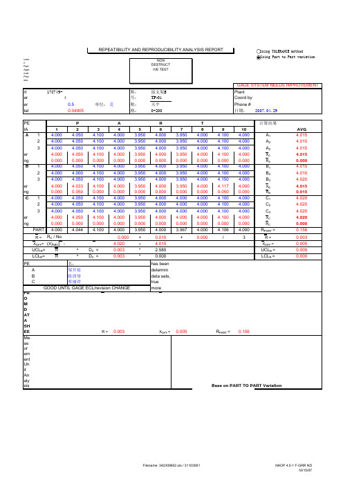
NON DESTRUCTIVE TEST'01 PSW '01 PSW'!A6'01 PSW'!A21'01 PSW'!A54'01 PSW'!H54GAGE SYSTEM NEEDS IMPROVEMENTPart number 8S79-17C749-A-PIA03/04零件名称:CD345焊接支架BPlant Characteristic 4 量具编号:TP-01 Coord by Tolerance0.5单位:克量具名称:天平 Phone #Total Variation (TV)0.04905量具规格:0-200日期:2007.04.29OPERATOR P A R T 计算结果TRIAL #12345678910AVG A 1 4.0004.050 4.100 4.000 3.950 4.000 3.950 4.000 4.100 4.000A 1 4.0152 4.0004.050 4.100 4.000 3.950 4.000 3.950 4.000 4.100 4.000A 2 4.01534.000 4.050 4.100 4.000 3.950 4.000 3.950 4.000 4.100 4.000A 34.015Average4.000 4.050 4.100 4.000 3.950 4.000 3.950 4.000 4.100 4.000X A 4.015Range 0.0000.0000.0000.0000.0000.0000.0000.0000.0000.000R A0.000B 14.000 4.050 4.100 4.000 3.950 4.000 3.950 4.000 4.100 4.000B 1 4.01524.000 4.000 4.100 4.000 3.950 4.000 3.950 4.000 4.100 4.000B 2 4.01034.000 4.050 4.100 4.000 3.950 4.000 3.950 4.000 4.150 4.000B 34.020Average 4.000 4.033 4.100 4.000 3.950 4.000 3.950 4.000 4.117 4.000X B 4.015Range 0.0000.0500.0000.0000.0000.0000.0000.0000.0500.000R B0.010C 14.000 4.050 4.100 4.000 3.950 4.000 4.000 4.000 4.100 4.000C 1 4.02024.000 4.050 4.100 4.000 3.950 4.000 4.000 4.000 4.100 4.000C 2 4.02034.000 4.050 4.100 4.000 3.950 4.000 4.000 4.000 4.100 4.000C 34.020Average 4.000 4.050 4.100 4.000 3.950 4.000 4.000 4.000 4.100 4.000X C 4.020Range0.0000.0000.0000.0000.0000.0000.0000.0000.0000.000R C0.000PART4.0004.0444.1004.000 3.950 4.000 3.967 4.000 4.106 4.000R PART =0.156R =R A + R B + R C / No of operators =0.000+0.010+0.000/3R =0.003X DIFF =[Max (X )ABC ] - [Min (X )ABC ] =4.020- 4.015X DIFF =0.005UCL R =R *D 4 =0.003* 2.580UCL R =0.009LCL R =R*D 3 =0.003*0.000LCL R =0.000OPERATOR 评价人姓名:NOTE : It has been statistically proven that the Tolerance Method is betterA 邹开琼to determine measurement equipment reliability. Even with negativeB 陈西琴Kurtosis data sets, the recorded measurements will be less than 1% awayC 邓丽君from the true value if GR&R is below 30%. Contact Quality Group if youGOOD UNTIL GAGE ECL/revision CHANGE need more information.FROM DATA SHEET:R =0.003X DIFF =0.005R PART =0.156Measurement Unit Analysis Base on PART TO PART Variation Repeatibility - Equipment Variation (EV)EV =R * K 1% EV = 100[EV/TV]EV =0.002Trials K 1% EV = 4.0230.5908Reproducibility - Appraiser Variation (AV)AV= [ ( X DIFF * K 2)2 - (EV 2 / nr)](n parts, r trials)% AV = 100[AV/TV]AV=0.003Oper K 2% AV = 5.2530.52Repeatibility & Reproducibility (R & R)% R&R = 100[R&R/TV]R&R= (EV 2 + AV 2)% R&R = 6.61R&R=0.003Part Variation (PV)PV=R PART * K 3Parts K 3% PV = 100[PV/TV]PV=0.049100.3146% PV =99.78Total Variation (TV)Based on PART VARIATIONTV= (R&R 2 + PV 2)#REF!GAGE IS REJECTED TV=0.049RANGES OUT OF UCLrNDC=21.2854Number of Distinct Data Categories(NDC)NDC=1.41* (PV/R&R)Guidelines for acceptance of gage repeatability and reproducibility (%R&R):UNDER 10% ERROR : Gage system OK10% to 30% ERROR:May be acceptable based upon importance of application. Calculate "breakpoint" = RPN x (% Gage R&R/100) andcheck that is less than 37.8 and (% Gage R&R) less than 30%. See next page for conclusion of usage.OVER 30% ERROR:Gage system needs improvement. Identify the problems and have them corrected.Using TOLERANCE methodUsing TOLERANCE methodNON DESTRUCTIVE TEST'01 PSW'01 PSW'!A6'01 PSW'!A21'01 PSW'!A54'01 PSW'!H54GAGE SYSTEM NEEDS IMPROVEMENT Part number8S79-17C749-A-PIA03/04零件名称:CD345焊接支架B PlantCharacteristic4量具编号:TP-01Coord byTolerance0.5单位:克量具名称:天平Phone #Total Variation (TV)0.04905量具规格:0-200日期:2007.04.29。
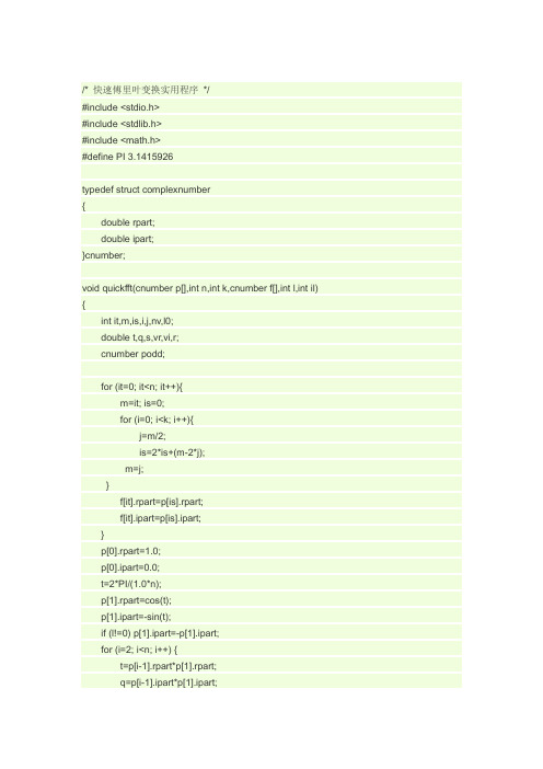
/* 快速傅里叶变换实用程序*/#include <stdio.h>#include <stdlib.h>#include <math.h>#define PI 3.1415926typedef struct complexnumber{double rpart;double ipart;}cnumber;void quickfft(cnumber p[],int n,int k,cnumber f[],int l,int il) {int it,m,is,i,j,nv,l0;double t,q,s,vr,vi,r;cnumber podd;for (it=0; it<n; it++){m=it; is=0;for (i=0; i<k; i++){j=m/2;is=2*is+(m-2*j);m=j;}f[it].rpart=p[is].rpart;f[it].ipart=p[is].ipart;}p[0].rpart=1.0;p[0].ipart=0.0;t=2*PI/(1.0*n);p[1].rpart=cos(t);p[1].ipart=-sin(t);if (l!=0) p[1].ipart=-p[1].ipart;for (i=2; i<n; i++) {t=p[i-1].rpart*p[1].rpart;q=p[i-1].ipart*p[1].ipart;s=(p[i-1].rpart+p[i-1].ipart)*(p[1].rpart+p[1].ipart);p[i].rpart=t-q; p[i].ipart=s-t-q;}for (it=0; it<n-1; it+=2){vr=f[it].rpart;vi=f[it].ipart;f[it].rpart=vr+f[it+1].rpart;f[it].ipart=vi+f[it+1].ipart;f[it+1].rpart=vr-f[it+1].rpart;f[it+1].ipart=vi-f[it+1].ipart;}m=n/2; nv=2;for (l0=k-2; l0>=0; l0--){m=m/2; nv=2*nv;for (it=0; it<=(m-1)*nv; it+=nv)for (j=0; j<=(nv/2)-1; j++) {t=p[m*j].rpart*f[it+j+nv/2].rpart;q=p[m*j].ipart*f[it+j+nv/2].ipart;s=p[m*j].rpart+p[m*j].ipart;s=s*(f[it+j+nv/2].rpart+f[it+j+nv/2].ipart);podd.rpart=t-q;podd.ipart=s-t-q;f[it+j+nv/2].rpart=f[it+j].rpart-podd.rpart;f[it+j+nv/2].ipart=f[it+j].ipart-podd.ipart;f[it+j].rpart=f[it+j].rpart+podd.rpart;f[it+j].ipart=f[it+j].ipart+podd.ipart;}}if (l!=0)for (i=0; i<n; i++){f[i].rpart/=n; f[i].ipart/=n;}if (il!=0)for (i=0; i<n; i++){p[i].rpart=sqrt(f[i].rpart*f[i].rpart+f[i].ipart*f[i].ipart);if (fabs(f[i].rpart)<0.000001*fabs(f[i].ipart)) {if ((f[i].ipart*f[i].rpart)>0) p[i].ipart=90.0;else p[i].ipart=-90.0;}elsep[i].ipart=atan(f[i].ipart/f[i].rpart)*360.0/(2*PI);}}int main(){int i,j;cnumber p[64],f[64];for (i=0; i<64; i++){p[i].rpart=exp(-0.1*(i+0.5));p[i].ipart=0.0;}printf("\n");for (i=0; i<8; i++){for (j=0; j<8; j++)printf("%2.5lf;",p[8*i+j].rpart);printf("\n");}printf("\n");quickfft(p,64,6,f,0,1);for (i=0; i<16; i++){for (j=0; j<4; j++){printf("%2.5lf",f[4*i+j].rpart);if(f[4*i+j].ipart<0) {printf("%2.5lfi;",f[4*i+j].ipart);}else {printf("+%2.5lfi;",f[4*i+j].ipart);}}printf("\n");}system("pause");return 0;}。

脑区英⽂及缩写Regions abbr.Precentral gyrus PreCG.L中央前回Precentral gyrus PreCG.R中央前回Superior frontal gyrus, dorsolateral SFGdor.L背外侧额上回Superior frontal gyrus, dorsolateral SFGdor.R背外侧额上回Superior frontal gyrus, orbital part ORBsup.L眶部额上回Superior frontal gyrus, orbital part ORBsup.R眶部额上回Middle frontal gyrus MFG.L额中回Middle frontal gyrus MFG.R额中回Middle frontal gyrus, orbital part ORBmid.L眶部额中回Middle frontal gyrus, orbital part ORBmid.R眶部额中回Inferior frontal gyrus, opercular part IFGoperc.L岛盖部额下回Inferior frontal gyrus, opercular part IFGoperc.R岛盖部额下回Inferior frontal gyrus, triangular part IFGtriang.L三⾓部额下回Inferior frontal gyrus, triangular part IFGtriang.R三⾓部额下回Inferior frontal gyrus, orbital part ORBinf.L眶部额下回Inferior frontal gyrus, orbital part ORBinf.R眶部额下回Rolandic operculum ROL.L中央沟盖Rolandic operculum ROL.R中央沟盖Supplementary motor area SMA.L补充运动区Supplementary motor area SMA.R补充运动区Olfactory cortex OLF.L嗅⽪质Olfactory cortex OLF.R嗅⽪质Superior frontal gyrus, medial SFGmed.L内侧额上回Superior frontal gyrus, medial SFGmed.R内侧额上回Superior frontal gyrus, medial orbital ORBsupmed.L眶内额上回Superior frontal gyrus, medial orbital ORBsupmed.R眶内额上回Gyrus rectus REC.L回直肌Gyrus rectus REC.R回直肌Insula INS.L脑岛Insula INS.R脑岛Anterior cingulate and paracingulate gyri ACG.L前扣带和旁扣带脑回Anterior cingulate and paracingulate gyri ACG.R前扣带和旁扣带脑回Median cingulate and paracingulate gyri DCG.L内侧和旁扣带脑回Median cingulate and paracingulate gyri DCG.R内侧和旁扣带脑回Posterior cingulate gyrus PCG.L后扣带回Posterior cingulate gyrus PCG.R后扣带回Hippocampus HIP.L海马Hippocampus HIP.R海马Parahippocampal gyrus PHG.L海马旁回Parahippocampal gyrus PHG.R海马旁回Amygdala AMYG.L杏仁核Amygdala AMYG.R杏仁核Calcarine fissure and surrounding cortex CAL.L距状裂周围⽪层Calcarine fissure and surrounding cortex CAL.R距状裂周围⽪层Cuneus CUN.L楔叶Cuneus CUN.R楔叶Lingual gyrus LING.L⾆回Lingual gyrus LING.R⾆回Superior occipital gyrus SOG.L枕上回Superior occipital gyrus SOG.R枕上回Middle occipital gyrus MOG.L枕中回Middle occipital gyrus MOG.R枕中回Inferior occipital gyrus IOG.L枕下回Inferior occipital gyrus IOG.R枕下回Fusiform gyrus FFG.L梭状回Fusiform gyrus FFG.R梭状回Postcentral gyrus PoCG.L中央后回Postcentral gyrus PoCG.R中央后回Superior parietal gyrus SPG.L顶上回Superior parietal gyrus SPG.R顶上回Inferior parietal, but supramarginal and angular gyri IPL.L顶下缘⾓回Inferior parietal, but supramarginal and angular gyri IPL.R顶下缘⾓回Supramarginal gyrus SMG.L缘上回Supramarginal gyrus SMG.R缘上回Angular gyrus ANG.L⾓回Angular gyrus ANG.R⾓回Precuneus PCUN.L楔前叶Precuneus PCUN.R楔前叶Paracentral lobule PCL.L中央旁⼩叶Paracentral lobule PCL.R中央旁⼩叶Caudate nucleus CAU.L尾状核Caudate nucleus CAU.R尾状核Lenticular nucleus, putamen PUT.L⾖状壳核Lenticular nucleus, putamen PUT.R⾖状壳核Lenticular nucleus, pallidum PAL.L⾖状苍⽩球Lenticular nucleus, pallidum PAL.R⾖状苍⽩球Thalamus THA.L丘脑Thalamus THA.R丘脑Heschl gyrus HES.L颞横回Heschl gyrus HES.R颞横回Superior temporal gyrus STG.L颞上回Superior temporal gyrus STG.R 颞上回Temporal pole: superior temporal gyrus TPOsup.L颞极:颞上回Temporal pole: superior temporal gyrus TPOsup.R颞极:颞上回Middle temporal gyrus MTG.L颞中回Middle temporal gyrus MTG.R颞中回Temporal pole: middle temporal gyrus TPOmid.L颞极:颞中回Temporal pole: middle temporal gyrus TPOmid.R颞极:颞中回Inferior temporal gyrus ITG.L颞下回Inferior temporal gyrus ITG.R颞下回和抑郁症相关和强迫症有关和强迫症有关中⽂处理和加⼯的关键部位,还具备通知记忆和不同信息协调功能,且其活动强度随⽂字复杂性的增加⽽逐渐增加,与⼯作记与⼯作记忆相关与AD有关科学家们在研究中发现,刺激⼤脑⽪层中央前回(⼜叫做第⼀运动区,)的顶部,可以引起下肢的运动;刺激中央前回的下部,则会出现头部器官的运动;刺激中央前回的其他部位,则会出现其他相应器官的运动。

【R】R语⾔常⽤包汇总⼀、⼀些函数包⼤汇总时间上有点过期,下⾯的资料供⼤家参考基本的R包已经实现了传统多元统计的很多功能,然⽽CRNA的许多其它包提供了更深⼊的多元统计⽅法,下⾯要综述的包主要分为以下⼏个部分:1)多元数据可视化(Visualising multivariate data)绘图⽅法 基本画图函数(如:pairs()、coplot())和 lattice包⾥的画图函数(xyplot()、splom())可以画成对列表的⼆维散点图,3维密度图。
car 包⾥的scatterplot.matrix()函数提供更强⼤的⼆维散点图的画法。
cwhmisc包集合⾥的cwhplot包的pltSplomT()函数类似pair()画散点图矩阵,⽽且可以在对⾓位置画柱状图或密度估计图。
除此之外,scatterplot3d包可画3维的散点图,aplpack包⾥bagplot()可画⼆变量的boxplot,spin3R()可画可旋转的三维点图。
misc3d包有可视化密度的函数。
YaleToolkit包提供许多多元数据可视化技术,agsemisc也是这样。
更特殊的多元图包括:aplpack包⾥的faces()可画Chernoff’s face;MASS包⾥的parcoord()可画平⾏坐标图(矩阵的每⼀⾏画⼀条线,横轴表⽰矩阵的每列); graphics包⾥的stars()可画多元数据的星状图(矩阵的每⼀⾏⽤⼀个星状图表⽰)。
ade4包⾥的mstree()和vegan包⾥的spantree()可画最⼩⽣成树。
calibrate包⽀持双变量图和散点图,chplot包可画convex hull图。
geometry包提供了和qhull库的接⼝,由convexhulln()可给出相应点的索引。
ellipse包可画椭圆,也可以⽤plotcorr()可视化相关矩阵。
denpro包为多元可视化提供⽔平集树形结构(level set trees)。


r语言机器算法代码以下是使用R语言实现常见的机器学习算法的示例代码:1. 线性回归(Linear Regression):```R# 使用lm函数进行线性回归model <- lm(y ~ x1 + x2, data=train_data)# 预测新数据点new_data <- data.frame(x1 = 5, x2 = 3) # 新数据点的特征值predicted <- predict(model, newdata=new_data)```2. 决策树(Decision Tree):```R# 使用rpart函数进行决策树构建model <- rpart(y ~ x1 + x2, data=train_data)# 预测新数据点new_data <- data.frame(x1 = 5, x2 = 3) # 新数据点的特征值predicted <- predict(model, newdata=new_data, type="class") ```3. 随机森林(Random Forest):```R# 使用randomForest包进行随机森林建模library(randomForest)# 构建随机森林模型model <- randomForest(y ~ x1 + x2, data=train_data)# 预测新数据点new_data <- data.frame(x1 = 5, x2 = 3) # 新数据点的特征值predicted <- predict(model, newdata=new_data)```4. K近邻算法(K-Nearest Neighbors):```R# 使用class包进行K近邻算法建模library(class)# 构建K近邻模型model <- knn(train = train_data[, c("x1", "x2")], test = test_data[, c("x1", "x2")], cl = train_data$y, k = 3)# 预测新数据点new_data <- data.frame(x1 = 5, x2 = 3) # 新数据点的特征值predicted <- knn(train = train_data[, c("x1", "x2")], test = new_data, cl = train_data$y, k = 3)```以上代码仅是示例,具体的实现可能需要根据实际数据和问题做相应的调整和修改。
15. 缺失值处理方法目录:一. 直接删除法二. 用均值/中位数/众数填补三. 探索变量的相关性插补四. 探索样本的相似性填补五. 分类树与回归树预测法插补(rpart包)六. 多重插补法(mice包)正文:一、直接删除法即直接删除含有缺失值的样本,有时最为简单有效,但前提是缺失数据的比例较少,且缺失数据是随机出现的,这样删除缺失数据后对分析结果影响不大。
1. 向量删除缺失值x<-c(1,2,3,NA,5)mean(x) #默认不忽略NA值或NaN值,注意与NULL的区别[1] NAmean(x,na.rm=TRUE) #忽略缺失值[1] 2.75x1<-x[!is.na(x)] #去掉向量中的NA值x1[1] 1 2 3 5x2<-na.omit(x) #返回去掉NA值的向量x2[1] 1 2 3 5attr(,"na.action")[1] 4attr(,"class")[1] "omit"na.fail(x) #若向量有NA值,则返回ErrorError in na.fail.default(x) : 对象里有遺漏值na.fail(x1) #若向量不含NA值,则返回该向量[1] 1 2 3 5attr(na.omit(x),"na.action") #返回向量中NA值的下标[1] 4attr(,"class")[1] "omit"x[is.na(x)]<-0 #将向量x中的NA值替换为0x[1] 1 2 3 0 52. 删除含缺失值的样本数据用DMwR包实现。
library(DMwR) #用自带数据集algae,18个变量,200个观测值library(VIM)sum(!complete.cases(algae)) #查看含有缺失值的样本个数[1] 16algae1<-na.omit(algae) #直接删除所有含缺失值的样本sum(!complete.cases(algae1))[1] 0#只删除缺失值过多的样本:缺失值个数大于列数的20%algae2<-algae[-manyNAs(algae,0.2),] #数据框的“删除行”操作sum(!complete.cases(algae2))其中,函数manyNAs(x,nORp)用来查找数据框x中缺失值过多(≥缺失比例nORp)的行;nORp默认为0.2,即缺失值个数≥列数的20%注:当删除缺失数据会改变数据结构时,通过对完整数据按照不同的权重进行加权,可以降低删除缺失数据带来的偏差。
模型验证⽅法——R语⾔在数据分析中经常会对不同的模型做判断⼀、混淆矩阵法作⽤:⼀种⽐较简单的模型验证⽅法,可算出不同模型的预测精度将模型的预测值与实际值组合成⼀个矩阵,正例⼀般是我们要预测的⽬标。
真正例就是预测为正例且实际也是正例(预测正确);假反例是实际是正例但模型错误预测成反例(即预测错误);假正例是预测是模型预测是正例,但实际是反例;真反例是预测是反例,实际也是反例。
查准率=真正例/假正例+真正例(真正率占我们预测是正例的⽐例)查全率=真正例/真正例+假反例(真正率占我们实际是正例的⽐例)混淆矩阵运⽤:以下以回归模型为例,探索混淆矩阵的使⽤# 设定五折交叉验证规则train_control<-trainControl(method = 'cv',number = 5)# 对数据集分成set.seed(1234)# 在任何随机事件之前都需要设定随机种⼦index<-createDataPartition(good_data$left,p=.7,list = F)head(index)traindata<-good_data[index, ]testdata<-good_data[-index, ]# 建⽴回归树模型rpart_model1<-train(left ~ .,data=traindata,trControl=train_control,method='rpart')# 将测试集导⼊回归树模型,求得测试结果pred_rpart<-predict(rpart_model1,testdata[-7])# 利⽤混淆矩阵对回归树模型进⾏评估con_rpart<-table(pred_rpart,testdata$left) # 混淆矩阵只⽤测试集,与训练集⽆关con_rpart # 求得混淆矩阵结果pred_rpart 0 10 2246 721 51 528对应查准率为:528/51+528=91.19%⼆、roc曲线模型验证,根据学习器的结果对样例排序,逐个把样本作为正例进⾏预测,每次计算出两个重要的值,分别以它们为横纵坐标作图,即得到ROC曲线。
公司部门英文缩写简称大全总公司H ead O ffice分公司Branc h Off ice营业部 Bu sines s Off ice人事部 Pe rsonn el De partm ent人力资源部Human Reso urces Depa rtmen t总务部 Gene ral A ffair s Dep artme nt财务部 Gen eralAccou nting Depa rtmen t销售部 Sale s Dep artme nt促销部 Sal es Pr omoti on De partm ent国际部 In terna tiona l Dep artme nt出口部 Exp ort D epart ment进口部I mport Depa rtmen t公共关系 Pub lic R elati ons D epart ment广告部A dvert ising Depa rtmen t企划部 Plan ningDepar tment产品开发部 Pro ductDevel opmen t Dep artme nt研发部 Res earch andDevel opmen t Dep artme nt(R&D) 秘书室 Sec retar ial P ool采购部 Pu rchas ing D epart ment工程部E ngine ering Depa rtmen t行政部 Admi n. De partm ent人力资源部HR De partm ent市场部 Ma rketi ng De partm ent技术部 Te chnol og De partm ent客服部 Se rvice Depa rtmen t行政部: Adm inist ratio n财务部 Fina ncial Depa rtmen t总经理室、Dir ecoto r, or Pres ident副总经理室、Dep uty D irect or, o r Vic e pre siden t总经办、Gene ral D eparm ent采购部、Pu rchas e & O rderDepar tment工程部、Engin eerin g Dep armen t研发部、Rese archDepar ment生产部、P roduc tiveDepar tment销售部、Sales Depa rment广东业务部、GDBranc h Dep armen t无线事业部、Wi reles s Ind ustry Depa rtmen t拓展部 Busi nessExpen dingDepar tment物供部、Suppl y Dep artme ntB&D bus iness anddevel opmen t 业务拓展部Ma rketi ng 市场部Sal es 销售部HR人力资源部Acco unt 会计部PR peop le re latio nship公共关系部OFC (Off ice,但不常见) / OM B = O ffice of M anage mentand B udget办公室Finan ce 财务部MKT G (Ma rketi ng) 市场部R&D (Re searc h & D evelo pment) 研发部MFG(Manu factu ring)产品部Admin istra tionDept.管理部Purch asing Dep t 采购部Chai rman/Presi dentOffic e //Gerne ral M anage r off ice o r GMoffic e 总经理办公室M onito r & S uppor t Dep artme nt 监事会Str ategy Rese arch战略研究部我认为翻译没有标准答案,要根据实际情况来进行决定。
An Introduction to Recursive PartitioningUsing the RPART RoutinesTerry M.TherneauElizabeth J.AtkinsonMayo FoundationMarch28,2014Contents1Introduction2 2Notation4 3Building the tree53.1Splitting criteria (5)3.2Incorporating losses (7)3.2.1Generalized Gini index (7)3.2.2Altered priors (8)3.3Example:Stage C prostate cancer(class method) (10)3.4Variable importance (11)4Pruning the tree124.1Definitions (12)4.2Cross-validation (13)4.3Example:The Stochastic Digit Recognition Problem (14)5Missing data185.1Choosing the split (18)5.2Surrogate variables (19)5.3Example:Stage C prostate cancer(cont.) (20)16Further options236.1Program options (23)6.2Example:Consumer Report Auto Data (25)6.3Example:Kyphosis data (30)7Regression337.1Definition (33)7.2Example:Consumer Report car data (34)7.3Example:Stage C data(anova method) (39)8Poisson regression428.1Definition (42)8.2Improving the method (43)8.3Example:solder data (44)8.4Example:Stage C Prostate cancer,survival method (48)8.5Open issues (49)9Plotting options52 10Other functions58 11Test Cases5911.1Classification (59)1IntroductionThis document is a modification of a technical report from the Mayo Clinic Division of Biostatistics[6],which was itself an expansion of an earlier Stanford report[5].It is intended to give a short overview of the methods found in the rpart routines,which implement many of the ideas found in the CART(Classification and Regression Trees)book and programs of Breiman,Friedman,Olshen and Stone[1].Because CART is the trademarked name of a particular software implementation of these ideas,and tree has been used for the S-Plus routines of Clark and Pregibon[2]a different acronym—Recursive PARTitioning or rpart—was chosen.It is somewhat humorous that this label“rpart”has now become more common than the original and more descriptive“cart”,a testament to the influence of freely available software.The rpart programs build classification or regression models of a very general structure using a two stage procedure;the resulting models can be represented as binary trees.An example is some preliminary data gathered at Stanford on revival of cardiac arrest patients by paramedics.The goal is to predict which patients can be successfully revived in thefield224revived 144not revivedr r rr r rr r r¨¨¨¨¨¨¨¨¨X 1=122/13X 1=2,3or 42/131¨¨¨¨¨r r rr rr rrr r¨¨¨¨¨X 2=120/5X 2=2or 32/8X 3=12/31X 3=2or 30/100Figure 1:Revival dataon the basis of fourteen variables known at or near the time of paramedic arrival,e.g.,sex,age,time from attack to first care,etc.Since some patients who are not revived on site are later successfully resuscitated at the hospital,early identification of these “recalcitrant”cases is of considerable clinical interest.The resultant model separated the patients into four groups as shown in figure 1,whereX 1=initial heart rhythm1=VF/VT 2=EMD 3=Asystole 4=Other X 2=initial response to defibrillation1=Improved 2=No change 3=Worse X 3=initial response to drugs1=Improved 2=No change 3=WorseThe other 11variables did not appear in the final model.This procedure seems to work especially well for variables such as X 1,where there is a definite ordering,but spacings are not necessarily equal.The tree is built by the following process:first the single variable is found which best splits the data into two groups (‘best’will be defined later).The data is separated,and then this process is applied separately to each sub-group,and so on recursively until the subgroups either reach a minimum size (5for this data)or until no improvement can be made.The resultant model is,with a certainty,too complex,and the question arises as it does with all stepwise procedures of when to stop.The second stage of the procedure consists of using cross-validation to trim back the full tree.In the medical example above the full tree3had ten terminal regions.A cross validated estimate of risk was computed for a nested set of sub trees;this final model was that sub tree with the lowest estimate of risk.2NotationThe partitioning method can be applied to many different kinds of data.We will start by looking at the classification problem,which is one of the more instructive cases (but also has the most complex equations).The sample population consists of n observations from C classes.A given model will break these observations into k terminal groups;to each of these groups is assigned a predicted class.In an actual application,most parameters will be estimated from the data,such estimates are given by ≈formulae.πi i =1,2,...,Cprior probabilities of each classL (i,j )i =1,2,...,C Loss matrix for incorrectly classifying an i as a j .L (i,i )≡0Asome node of the treeNote that A represents both a set of individuals in the sample data,and,via the tree that produced it,a classification rule for future data.τ(x )true class of an observation x ,where x is the vector of predictor variablesτ(A )the class assigned to A,if A were to be taken as a final noden i ,n Anumber of observations in the sample that are class i ,number of obs in node AP (A )probability of A (for future observations)= C i =1πi P {x ∈A |τ(x )=i }≈ Ci =1πi n iA /n ip (i |A )P {τ(x )=i |x ∈A }(for future observations)=πi P {x ∈A |τ(x )=i }/P {x ∈A }≈πi (n iA /n i )/ πi (n iA /n i )4R (A )risk of A = C i =1p (i |A )L (i,τ(A ))where τ(A )is chosen to minimize this risk R (T )risk of a model (or tree)T = k j =1P (A j )R (A j )where A j are the terminal nodes of the treeIf L (i,j )=1for all i =j ,and we set the prior probabilities πequal to the observed class frequencies in the sample then p (i |A )=n iA /n A and R (T )is the proportion misclassified.3Building the tree3.1Splitting criteriaIf we split a node A into two sons A L and A R (left and right sons),we will haveP (A L )r (A L )+P (A R )r (A R )≤P (A )r (A )(this is proven in [1]).Using this,one obvious way to build a tree is to choose that split which maximizes ∆r ,the decrease in risk.There are defects with this,however,as the following example shows:Suppose losses are equal and that the data is 80%class 1’s,and that some trial split results in A L being 54%class 1’s and A R being 100%class 1’s.Since the minimum risk prediction for both the left and right son is τ(A L )=τ(A R )=1,this split will have ∆r =0,yet scientifically this is a very informative division of the sample.In real data with such a majority,the first few splits very often can do no better than this.A more serious defect is that the risk reduction is essentially linear.If there were two competing splits,one separating the data into groups of 85%and 50%purity respectively,and the other into 70%-70%,we would usually prefer the former,if for no other reason than because it better sets things up for the next splits.One way around both of these problems is to use look-ahead rules;but these are com-putationally very expensive.Instead rpart uses one of several measures of impurity,or diversity,of a node.Let f be some impurity function and define the impurity of a node A asI (A )=Ci =1f (p iA )50.00.20.40.60.8 1.00.00.10.20.30.40.50.60.7PI m p u r i t yGiniInformation rescaled GiniFigure 2:Comparison of Gini and Information impurity for two groups.where p iA is the proportion of those in A that belong to class i for future samples.Since we would like I (A )=0when A is pure,f must be concave with f (0)=f (1)=0.Two candidates for f are the information index f (p )=−p log(p )and the Gini index f (p )=p (1−p ).We then use that split with maximal impurity reduction∆I =p (A )I (A )−p (A L )I (A L )−p (A R )I (A R )The two impurity functions are plotted in figure (2),along with a rescaled version of the Gini measure.For the two class problem the measures differ only slightly,and will nearly always choose the same split point.Another convex criteria not quite of the above class is twoing for whichI (A )=min C 1C 2[f (p C 1)+f (p C 2)]where C 1,C 2is some partition of the C classes into two disjoint sets.If C =2twoing is equivalent to the usual impurity index for f .Surprisingly,twoing can be calculated almost as efficiently as the usual impurity index.One potential advantage of twoing is that6the output may give the user additional insight concerning the structure of the data.It can be viewed as the partition of C into two superclasses which are in some sense the most dissimilar for those observations in A .For certain problems there may be a natural ordering of the response categories (e.g.level of education),in which case ordered twoing can be naturally defined,by restricting C 1to be an interval [1,2,...,k ]of classes.Twoing is not part of rpart .3.2Incorporating lossesOne salutatory aspect of the risk reduction criteria not found in the impurity measures is inclusion of the loss function.Two different ways of extending the impurity criteria to also include losses are implemented in CART,the generalized Gini index and altered priors.The rpart software implements only the altered priors method.3.2.1Generalized Gini indexThe Gini index has the following interesting interpretation.Suppose an object is selected at random from one of C classes according to the probabilities (p 1,p 2,...,p C )and is randomly assigned to a class using the same distribution.The probability of misclassification isij =ip i p j = ijp i p j − ip 2i =i1−p 2i =Gini index for pLet L (i,j )be the loss of assigning class j to an object which actually belongs to class i .The expected cost of misclassification isL (i,j )p i p j .This suggests defining a generalized Gini index of impurity by G (p )= ijL (i,j )p i p jThe corresponding splitting criterion appears to be promising for applications involvingvariable misclassification costs.But there are several reasonable objections to it.First,G (p )is not necessarily a concave function of p ,which was the motivating factor behind impurity measures.More seriously,G symmetrizes the loss matrix before using it.To see this note that G (p )=(1/2)[L (i,j )+L (j,i )]p i p j In particular,for two-class problems,G in effect ignores the loss matrix.73.2.2Altered priorsRemember the definition of R (A )R (A )≡C i =1p iA L (i,τ(A ))=C i =1πi L (i,τ(A ))(n iA /n i )(n/n A )Assume there exists ˜πand ˜Lbe such that ˜πi ˜L(i,j )=πi L (i,j )∀i,j ∈CThen R (A )is unchanged under the new losses and priors.If ˜Lis proportional to the zero-one loss matrix then the priors ˜πshould be used in the splitting criteria.This is possible only if L is of the form L (i,j )=L i i =j0i =j in which case˜πi =πi L ij πj L jThis is always possible when C =2,and hence altered priors are exact for the two class problem.For arbitrary loss matrix of dimension C >2,rpart uses the above formula with L i = j L (i,j ).A second justification for altered priors is this.An impurity index I (A )=f (p i )has its maximum at p 1=p 2=...=p C =1/C .If a problem had,for instance,a misclassification loss for class 1which was twice the loss for a class 2or 3observation,one would wish I(A)to have its maximum at p 1=1/5,p 2=p 3=2/5,since this is the worst possible set of proportions on which to decide a node’s class.The altered priors technique does exactly this,by shifting the p i .Two final notes•When altered priors are used,they affect only the choice of split.The ordinary losses and priors are used to compute the risk of the node.The altered priors simply help the impurity rule choose splits that are likely to be “good”in terms of the risk.•The argument for altered priors is valid for both the Gini and information splitting rules.8|grade< 2.5g2< 13.2ploidy=ab g2>=11.84g2< 11g2>=17.91age>=62.5NoNoNoProgNoProgProgFigure 3:Classification tree for the Stage C data93.3Example:Stage C prostate cancer(class method)Thisfirst example is based on a data set of146stage C prostate cancer patients[4].The main clinical endpoint of interest is whether the disease recurs after initial surgical removalof the prostate,and the time interval to that progression(if any).The endpoint in this example is status,which takes on the value1if the disease has progressed and0if not. Later we’ll analyze the data using the exp method,which will take into account time to progression.A short description of each of the variables is listed below.The main predictor variable of interest in this study was DNA ploidy,as determined byflow cytometry.For diploid and tetraploid tumors,theflow cytometry method was also able to estimate the percent of tumor cells in a G2(growth)stage of their cell cycle;G2%is systematically missing for most aneuploid tumors.The variables in the data set arepgtime time to progression,or last follow-up free of progressionpgstat status at last follow-up(1=progressed,0=censored)age age at diagnosiseet early endocrine therapy(1=no,0=yes)ploidy diploid/tetraploid/aneuploid DNA patterng2%of cells in G2phasegrade tumor grade(1-4)gleason Gleason grade(3-10)The model isfit by using the rpart function.Thefirst argument of the function is a model formula,with the∼symbol standing for“is modeled as”.The print function givesan abbreviated output,as for other S models.The plot and text command plot the tree and then label the plot,the result is shown infigure3.>progstat<-factor(stagec$pgstat,levels=0:1,labels=c("No","Prog")) >cfit<-rpart(progstat~age+eet+g2+grade+gleason+ploidy,data=stagec,method='class')>print(cfit)n=146node),split,n,loss,yval,(yprob)*denotes terminal node1)root14654No(0.63013700.3698630)2)grade<2.5619No(0.85245900.1475410)*3)grade>=2.58540Prog(0.47058820.5294118)6)g2<13.24017No(0.57500000.4250000)12)ploidy=diploid,tetraploid3111No(0.64516130.3548387)1024)g2>=11.84571No(0.85714290.1428571)*25)g2<11.8452410No(0.58333330.4166667)50)g2<11.005175No(0.70588240.2941176)*51)g2>=11.00572Prog(0.28571430.7142857)*13)ploidy=aneuploid93Prog(0.33333330.6666667)*7)g2>=13.24517Prog(0.37777780.6222222)14)g2>=17.91228No(0.63636360.3636364)28)age>=62.5154No(0.73333330.2666667)*29)age<62.573Prog(0.42857140.5714286)*15)g2<17.91233Prog(0.13043480.8695652)*>par(mar=rep(0.1,4))>plot(cfit)>text(cfit)•The creation of a labeled factor variable as the response improves the labeling of the printout.•We have explicitly directed the routine to treat progstat as a categorical variable by asking for method=’class’.(Since progstat is a factor this would have been the default choice).Since no optional classification parameters are specified the routine will use the Gini rule for splitting,prior probabilities that are proportional to the observed data frequencies,and0/1losses.•The child nodes of node x are always2x and2x+1,to help in navigating the printout (compare the printout tofigure3).•Other items in the list are the definition of the split used to create a node,the number of subjects at the node,the loss or error at the node(for this example,with proportional priors and unit losses this will be the number misclassified),and the predicted class for the node.•*indicates that the node is terminal.•Grades1and2go to the left,grades3and4go to the right.The tree is arranged so that the branches with the largest“average class”go to the right.3.4Variable importanceThe long form of the printout for the stage C data,obtained with the summary function, contains further information on the surrogates.The cp option of the summary function instructs it to prune the printout,but it does not prune the tree.For each node up to511surrogate splits (default)will be printed,but only those whose utility is greater than the baseline “go with the majority”surrogate.The first surrogate for the first split is based on the following table:>temp <-with(stagec,table(cut(grade,c(0,2.5,4)),cut(gleason,c(2,5.5,10)),exclude =NULL))>temp(2,5.5](5.5,10]<NA>(0,2.5]42163(2.5,4]1840<NA>000The surrogate sends 126of the 146observations the correct direction for an agreement of 0.863.The majority rule gets 85correct,and the adjusted agreement is (126-85)/(146-85).A variable may appear in the tree many times,either as a primary or a surrogate variable.An overall measure of variable importance is the sum of the goodness of split measures for each split for which it was the primary variable,plus goodness *(adjusted agreement)for all splits in which it was a surrogate.In the printout these are scaled to sum to 100and the rounded values are shown,omitting any variable whose proportion is less than 1%.Imagine two variables which were essentially duplicates of each other;if we did not count surrogates they would split the importance with neither showing up as strongly as it should.4Pruning the tree 4.1DefinitionsWe have built a complete tree,possibly quite large and/or complex,and must now decide how much of that model to retain.In stepwise regression,for instance,this issue is addressed sequentially and the fit is stopped when the F test fails to achieve some level α.Let T 1,T 2,....,T k be the terminal nodes of a tree T.Define|T |=number of terminal nodes risk of T =R (T )= k i =1P (T i )R (T i )In comparison to regression,|T |is analogous to the degrees of freedom and R (T )to the residual sum of squares.Now let αbe some number between 0and ∞which measures the ’cost’of adding another variable to the model;αwill be called a complexity parameter.Let R (T 0)be the risk for12the zero split tree.DefineR α(T )=R (T )+α|T |to be the cost for the tree,and define T αto be that sub tree of the full model which has minimal cost.Obviously T 0=the full model and T ∞=the model with no splits at all.The following results are shown in [1].1.If T 1and T 2are sub trees of T with R α(T 1)=R α(T 2),then either T 1is a sub tree of T 2or T 2is a sub tree of T 1;hence either |T 1|<|T 2|or |T 2|<|T 1|.2.If α>βthen either T α=T βor T αis a strict sub tree of T β.3.Given some set of numbers α1,α2,...,αm ;both T α1,...,T αm and R (T α1),...,R (T αm )can be computed efficiently.Using the first result,we can uniquely define T αas the smallest tree T for which R α(T )is minimized.Since any sequence of nested trees based on T has at most |T |members,result 2implies that all possible values of αcan be grouped into m intervals,m ≤|T |I 1=[0,α1]I 2=(α1,α2]...I m =(αm −1,∞]where all α∈I i share the same minimizing sub tree.4.2Cross-validationCross-validation is used to choose a best value for αby the following steps:1.Fit the full model on the data setcompute I 1,I 2,...,I mset β1=0β2=√α1α2β3=√α2α3...βm −1=√αm −2αm −1βm =∞each βi is a ‘typical value’for its I i132.Divide the data set into s groups G1,G2,...,G s each of size s/n,and for each groupseparately:•fit a full model on the data set‘everyone except G i’and determine Tβ1,Tβ2,...,Tβmfor this reduced data set,•compute the predicted class for each observation in G i,under each of the modelsTβjfor1≤j≤m,•from this compute the risk for each subject.3.Sum over the G i to get an estimate of risk for eachβj.For thatβ(complexityparameter)with smallest risk compute Tβfor the full data set,this is chosen as the best trimmed tree.In actual practice,we may use instead the1-SE rule.A plot ofβversus risk often has an initial sharp drop followed by a relativelyflat plateau and then a slow rise.The choice ofβamong those models on the plateau can be essentially random.To avoid this,both an estimate of the risk and its standard error are computed during the cross-validation.Any risk within one standard error of the achieved minimum is marked as being equivalent to the minimum(i.e.considered to be part of theflat plateau).Then the simplest model, among all those“tied”on the plateau,is chosen.In the usual definition of cross-validation we would have taken s=n above,i.e.,each of the G i would contain exactly one observation,but for moderate n this is computationally prohibitive.A value of s=10has been found to be sufficient,but users can vary this if they wish.In Monte-Carlo trials,this method of pruning has proven very reliable for screening out ‘pure noise’variables in the data set.4.3Example:The Stochastic Digit Recognition ProblemThis example is found in section2.6of[1],and used as a running example throughout much of their book.Consider the segments of an unreliable digital readout141745236where each light is correct with probability 0.9,e.g.,if the true digit is a 2,the lights 1,3,4,5,and 7are on with probability 0.9and lights 2and 6are on with probability 0.1.Construct test data where Y ∈{0,1,...,9},each with proportion 1/10and the X i ,i =1,...,7are i.i.d.Bernoulli variables with parameter depending on Y.X 8−X 24are generated as i.i.d Bernoulli P {X i =1}=.5,and are independent of Y.They correspond to embedding the readout in a larger rectangle of random lights.A sample of size 200was generated accordingly and the procedure applied using the Gini index (see 3.2.1)to build the tree.The S code to compute the simulated data and the fit are shown below.>set.seed(1953)#An auspicious year >n <-200>y <-rep(0:9,length =200)>temp <-c(1,1,1,0,1,1,1,0,0,1,0,0,1,0,1,0,1,1,1,0,1,1,0,1,1,0,1,1,0,1,1,1,0,1,0,1,1,0,1,0,1,1,0,1,0,1,1,1,1,1,0,1,0,0,1,0,1,1,1,1,1,1,1,1,1,1,1,0,1,0)>lights <-matrix(temp,10,7,byrow =TRUE)#The true light pattern 0-9>temp1<-matrix(rbinom(n*7,1,0.9),n,7)#Noisy lights>temp1<-ifelse(lights[y+1,]==1,temp1,1-temp1)>temp2<-matrix(rbinom(n*17,1,0.5),n,17)#Random lights>x <-cbind(temp1,temp2)15|x3>=0.5x1< 0.5x4< 0.5x2< 0.5x5>=0.5x4>=0.5x4< 0.5x7>=0.5 x5< 0.5x1>=0.514237956 Figure4:Optimally pruned tree for the stochastic digit recognition data16>dfit<-rpart(y~x,method='class',control=rpart.control(xval=10,minbucket=2,cp=0)) >printcp(dfit)Classification tree:rpart(formula=y~x,method="class",control=rpart.control(xval=10, minbucket=2,cp=0))Variables actually used in tree construction:[1]x1x10x13x14x17x19x2x21x3x4x5x6x7x8[15]x9Root node error:180/200=0.9n=200CP nsplit rel error xerror xstd10.11111110 1.000001.105560.005541620.100000010.888890.983330.025064730.088888920.788890.883330.031717840.077777840.611110.816670.034674450.066666750.533330.694440.038036360.061111160.466670.666670.038490070.055555670.405560.638890.038839380.038888980.350000.466670.038777690.022222290.311110.394440.0375956100.0166667100.288890.372220.0370831110.0083333110.272220.366670.0369434120.0055556170.222220.372220.0370831130.0027778250.177780.361110.0367990140.0000000270.172220.350000.0364958>fit9<-prune(dfit,cp=0.02)>par(mar=rep(0.1,4))>plot(fit9,branch=0.3,compress=TRUE)>text(fit9)This table differs from that in section3.5of[1]in several ways,the last two of whichare substantive.•The actual values are different,of course,because of different random number gener-ators in the two runs.17•The complexity table is printed from the smallest tree(no splits)to the largest one (28splits).Wefind it easier to compare one tree to another when they start at the same place.•The number of splits is listed,rather than the number of nodes.The number of nodes is always1+the number of splits.•For easier reading,the error columns have been scaled so that thefirst node has an error of1.Since in this example the model with no splits must make180/200 misclassifications,multiply columns3-5by180to get a result in terms of absolute error.(Computations are done on the absolute error scale,and printed on relative scale).•The complexity parameter column has been similarly scaled.Looking at the table,we see that the best tree has10terminal nodes(9splits),based on cross-validation.This sub tree is extracted with a call to prune and saved in fit9.The pruned tree is shown infigure4.Two options have been used in the plot.The compress option tries to narrow the printout by vertically overlapping portions of the plot.The branch option controls the shape of the branches that connect a node to its children.The largest tree,with35terminal nodes,correctly classifies170/200=85%of the observations,but uses several of the random predictors in doing so and seriously overfits the data.If the number of observations per terminal node(minbucket)had been set to1 instead of2,then every observation would be classified correctly in thefinal model,many in terminal nodes of size1.5Missing data5.1Choosing the splitMissing values are one of the curses of statistical models and analysis.Most procedures deal with them by refusing to deal with them–incomplete observations are tossed out.Rpart is somewhat more ambitious.Any observation with values for the dependent variable and at least one independent variable will participate in the modeling.The quantity to be maximized is still∆I=p(A)I(A)−p(A L)I(A L)−p(A R)I(A R)The leading term is the same for all variables and splits irrespective of missing data,but the right two terms are somewhat modified.Firstly,the impurity indices I(A R)and I(A L) are calculated only over the observations which are not missing a particular predictor. Secondly,the two probabilities p(A L)and p(A R)are also calculated only over the relevant18observations,but they are then adjusted so that they sum to p(A).This entails some extra bookkeeping as the tree is built,but ensures that the terminal node probabilities sum to1.In the extreme case of a variable for which only2observations are non-missing,the impurity of the two sons will both be zero when splitting on that variable.Hence∆I will be maximal,and this‘almost all missing’coordinate is guaranteed to be chosen as best; the method is certainlyflawed in this extreme case.It is difficult to say whether this bias toward missing coordinates carries through to the non-extreme cases,however,since a more complete variable also affords for itself more possible values at which to split.5.2Surrogate variablesOnce a splitting variable and a split point for it have been decided,what is to be done with observations missing that variable?One approach is to estimate the missing datum using the other independent variables;rpart uses a variation of this to define surrogate variables.As an example,assume that the split(age<40,age≥40)has been chosen.The surrogate variables are found by re-applying the partitioning algorithm(without recursion)to predict the two categories‘age<40’vs.‘age≥40’using the other independent variables.For each predictor an optimal split point and a misclassification error are computed. (Losses and priors do not enter in—none are defined for the age groups—so the risk is simply#misclassified/n.)Also evaluated is the blind rule‘go with the majority’which has misclassification error min(p,1−p)wherep=(#in A with age<40)/n A.The surrogates are ranked,and any variables which do no better than the blind rule are discarded from the list.Assume that the majority of subjects have age≤40and that there is another variable x which is uncorrelated to age;however,the subject with the largest value of x is also over 40years of age.Then the surrogate variable x<max versus x≥max will have one less error that the blind rule,sending1subject to the right and n−1to the left.A continuous variable that is completely unrelated to age has probability1−p2of generating such a trim-one-end surrogate by chance alone.For this reason the rpart routines impose one more constraint during the construction of the surrogates:a candidate split must send at least2observations to the left and at least2to the right.Any observation which is missing the split variable is then classified using thefirst sur-rogate variable,or if missing that,the second surrogate is used,and etc.If an observation is missing all the surrogates the blind rule is used.Other strategies for these‘missing every-thing’observations can be convincingly argued,but there should be few or no observations of this type(we hope).19。