GIS, Users, Developers, and Spatial Statistics On Monarchs and Their Clothing
- 格式:pdf
- 大小:290.06 KB
- 文档页数:18

国内外常用两个GIS平台软件介绍摘要:地理信息系统(Geographic Information System, 简称GIS)地理信息系统是以地理空间数据库为基础,在计算机软硬件的支持下,运用系统工程和信息科学的理论,科学管理和综合分析具有空间内涵的地理数据,以提供管理、决策等所需信息的技术系统。
简单的说,GIS是综合处理和分析地理空间数据的一种技术系统,是以测绘测量为基础,以数据库作为数据储存和使用的数据源,以计算机编程为平台的全球空间分析即时技术。
作为获取、处理、管理和分析地理空间数据的重要工具、技术和学科,近年来得到了广泛关注和迅猛发展。
目前GIS已经快速的应用到各个领域,发展速度非常快,好多高校相应也开设了相关专业。
国外的常用的GIS软件有AutoCAD Map3d、ArcGIS、MapInfo等,而国内比较知名的GIS软件则是Supermap、MapGIS、GeoStar等。
本文将选取GeoMap 和MapInfo两款软件,进行相关介绍以及功能介绍。
关键词:GIS;GeoMap;MapInfo;功能介绍Introductionof two GIS platform softwares at home andabroadAbstract : Geographic Information Systems (Geographic Information System, referred to as GIS) geographic information system is based on geo-spatial databases , with the support of computer hardware and software , the use of the theory of systems engineering and information science , scientific management and comprehensive analysis of spatial connotation geographic data to provide the necessary information technology systems management and decision-making. Simply put , GIS is a comprehensive geospatial data processing and analysis of a technical system that is based on the measurement -based mapping to the database as a data storage and data sources used in computer programming as a platform for the analysis of real-time global space technology . As access to important tools, techniques and disciplines processing, management and analysis of geospatial data has been widespread concern in recent years and rapid development. Currently GIS has been applied to all areas of rapid development speed is very fast , a lot of colleges and universities have set up the appropriate relevant professional . GIS software used abroad have AutoCAD Map3d, ArcGIS, MapInfo , etc., and more well-known domestic GIS software is Supermap, MapGIS, GeoStar and so on. This article will select two GeoMap and MapInfo software, related presentations and Features .Key words:GIS GeoMap MapInfo Introduction of Function引言:地理信息系统(Geographic Information System或 Geo-Information system,简称GIS)是用于回答具有物质属性和空间坐标且与时间相关联问题的艺术、科学、工程和技术的统称,是集计算机科学、地理科学、测绘科学、环境科学、城市科学、空间科学、信息科学和管理科学为一体的新兴边缘学科。

ArcGIS Spatial Analyst栅格数据和非栅格数据的复合应用是GIS应用中的一个趋势,目前多数GIS软件关注的是矢量数据的分析和应用。
随着GIS和遥感以及DEM的不断发展,栅格数据在GIS中将扮演越来越重要的角色。
第一节空间分析扩展模块简介1.1 简介ArcGIS空间分析扩展模块提供了功能强大的空间建模和分析工具。
利用这个扩展模块可以创建基于栅格的数据,并对其查询,分析,绘图。
在空间分析模块中我们可以采用的数据包括影像,Grid以及其他的栅格数据集。
1.2 空间分析扩展模块功能下面列举一些使用该模块可以实现的功能:· 根据要素生成Arcinfo Grid·从要素按照一定距离或临近关系生成Raster· 由点状要素生成密度栅格图· 由离散要素点生成连续表面· 根据要素派生出等高线,坡度图,坡向图和山体阴影· 进行基于栅格数据的分析· 同时在多个栅格数据上进行逻辑查询和代数运算· 进行临域和区域分析· 进行栅格分类和显示· 支持很多标准格式1.3 空间模型模型就是把源域的组成部分表现在目标域中的一种结构。
源域中被表现的部分可以是实体,关系,过程或者其他感兴趣的现象。
建模的目的就是对源域的简单化和抽象化。
因此空间建模就是对地面上的地理实体进行简单和抽象化进行表示的过程。
模型有两类:表征模型和过程模型。
前者是用来描述物体,而后者则关注是物体间的相互作用和描述过程。
GIS过程模型,它可以使用一个流程图来表示。
第二节在ArcGIS中进行空间分析2.1分析环境设置在进行空间分析前,必须对设定分析范围,存储形式,存储使用的坐标系统,输出Grid的大小,缺省的输出目录。
下面将一一对此进行说明(这些设置是在Sptial Analyst工具条---->Spatial Analyst菜单---->Options中设置)坐标系统和矢量数据类似,没有校准的栅格数据是没有太大使用价值的。
ArcGIS教程:Spatial Analyst 扩展模块ArcGIS Spatial Analyst 扩展模块提供了多种强大的空间建模与分析功能。
如:创建、查询和分析基于像元的栅格数据并基于这些数据制图;将栅格/矢量分析进行整合;从现有数据中获取新信息;在多个数据图层中查询信息;将基于像元的栅格数据与传统的矢量数据源完全整合。
应用示例Spatial Analyst 能够帮助您实现多种功能,其中包括:从现有数据中获取新信息。
应用 Spatial Analyst 工具可基于源数据创建有价值的信息。
您能够实现的任务包括:基于点、折线或面数据得到距离;根据特定位置的测量数据计算出人口密度;将现有数据按适宜性重新分类;基于高程数据创建坡度、坡向或山体阴影。
查找适宜位置。
通过合并信息图层,针对特定目的查找最适宜的区域(例如,为建筑物选址,分析洪水或泥石流高风险区域)。
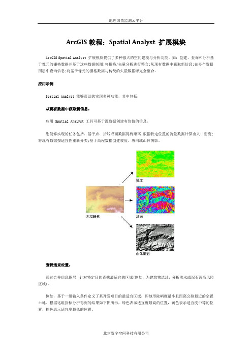
例如,基于一组输入条件定义了某开发项目的最适宜区域,即地形陡峭度最小且距离公路最近的空置土地。
根据这组指标分析得到的结果如下图所示,绿色表示适宜度最高的位置,黄色表示适宜度中等的位置,棕色表示适宜度最低的位置。
执行距离和行程成本分析。
创建欧氏距离表面以推算两个位置间的直线距离,或者创建成本加权距离表面以根据一组指定的输入条件来推算从一个位置到另一个位置所需的成本。
您可以计算从任意位置(像元)到最近的源位置的直线距离,也可以计算从任意位置到最近的源位置的所需成本。
确定两个位置间的最佳路径。
在考虑经济、环境和其他条件因素的前提下,为道路规划、管线铺设或动物迁移确定最佳路径或最适宜的廊道。
最短路径不一定就是成本最低的路径,可能会有若干个备选廊道可供采纳。
根据当地环境、较小邻域或预先确定的区域执行统计分析。
基于每个像元值对跨多个栅格的数据进行计算,例如,计算 10 年间的作物平均产量。
通过计算某邻域内包含的物种种类等特性对该邻域进行研究。
确定每个区域的平均值,例如,每个森林区的平均高程值。

地理信息系统英文专业名词English:Geographic Information System (GIS) is a system designed to capture, store, manipulate, analyze, manage, and present spatial or geographic data. It allows users to view, understand, question, interpret, and visualize data in many ways that reveal relationships, patterns, and trends in the form of maps, globes, reports, and charts. Key components of a GIS include hardware, software, data, and people. Examples of geographic information system software include QGIS, ArcGIS, and Google Earth. GIS is widely used in various fields such as urban planning, environmental resource management, natural resource management, archaeology, and public health.中文翻译:地理信息系统(GIS)是一个旨在捕获、存储、操纵、分析、管理和呈现空间或地理数据的系统。
它允许用户以多种方式查看、了解、提问、解释和可视化数据,揭示地图、地球仪、报告和图表形式上的关系、模式和趋势。
地理信息系统的关键组成部分包括硬件、软件、数据和人员。
地理信息系统软件的例子包括QGIS、ArcGIS和Google Earth。

手把手教你做g i s地形分析本页仅作为文档封面,使用时可以删除This document is for reference only-rar21year.March用gis做地形分析一、准备工作:1.拥有授权过(破解过的)软件;2.拥有一个DWG文件(其中需要有高程点的图层);3.认真按照这个文章的步骤做;4.参照以上三点。
二、含高程点DWG文件准备1.首先,找到你需要分析高程(坡度、坡向等)的DWG源文件。
打开后,如图所示。
2.随意找到一个高程点,仔细观察CAD软件左下角的Z坐标是否为0,不为0,且有一定的数值,则请看第三步。
如果没有Z坐标的值,则看下面的红色字体。
因为这次选用的CAD文件的高程点是没有值的,所以要利用湘源控规\飞时达来解决这个问题,下面分别进行介绍。
(1)打开飞时达,打开有高程点的CAD文件,除了高程点图层,在图层管理器中关闭其他所有的图层。
使用飞时达的“地形——高程点转换——输入最小有效高程值〈不限制〉——输入最大有效高程值〈不限制〉——选择一个高程点——该图元已有标高,是否直接采用〈Y〉——是否生成标高文字〈N〉——转换同类型图元〈A〉——确定”。
(2)打开湘源,打开有高程点的CAD文件,除了高程点图层,在图层管理器中关闭其他所有的图层。
使用湘源的“地形——字转高程——标高最低值0——标高最高值100——是否过滤小数点选择1——框选所有高程点——确定”。
按照这个步骤后,我们可以看到所有的高程点的Z值已经生成了。
将转好高程值的DWG文件,放至“文档——ArcGis文件夹”。
PS:请大家养成好习惯,所有gis要用到的文件夹和文件一定不能用汉字命名,作者经常碰到错误是因为这类习惯造成的,此外,尽量在磁盘根目录下新建文件夹用来进行GIS分析,因为这样好找。
3.打开GIS软件(ArcMap)。
如图所示:4.打开GIS后,先确认你的Spatial模块是否开启。
点击“自定义——扩展模块”,检查里面的spatial analyst 是否开启,作者为了方便,全部都勾选了,反正不影响系统速度。
《专业英语》课程教学大纲课程名称(中文/英文):专业英语/ Professional English 课程编码:12024019 课程类型:专业选修课 课程性质:专业课 适用范围:06地理信息系统学分数:2 先修课程:《大学英语》《地理信息系统》 学时数:36 其中:实验/实践学时:0 课外学时:0 考核方式:考查 制订日期:2006年制订单位:广州大学地理科学学院 审核者:夏丽华 执笔者:冯艳芬一、教学大纲说明(一)课程的地位、作用和任务(一)课程的地位、作用和任务该课程属于地理信息系统专业基础课之一,通过该课程的学习,学生基本能掌握常用的地理信息系统专业词汇,能查阅相关的外文资料,阅读简单的外文文献,阅读简单的外文文献,能进行简单的英文能进行简单的英文摘要撰写。
摘要撰写。
本课程的任务主要为:本课程的任务主要为:(1) 增加学生专业词汇量增加学生专业词汇量 (2) 介绍专业文献阅读的技巧介绍专业文献阅读的技巧 (3) 加强对英文长句翻译的训练加强对英文长句翻译的训练 (4) 介绍论文英文摘要的写法介绍论文英文摘要的写法(5) 介绍专业在国际上的发展趋势介绍专业在国际上的发展趋势 (二)课程教学的目的和要求(二)课程教学的目的和要求能让学生在学完二年能让学生在学完二年《大学英语》的基础上,《大学英语》的基础上,《大学英语》的基础上,增加专业方面的词汇,同时了解本专业在增加专业方面的词汇,同时了解本专业在英文上的表达方式,通过本课程的学习,通过本课程的学习,学生能掌握较多的专业词汇,学生能掌握较多的专业词汇,学生能掌握较多的专业词汇,能根据教学的要求查能根据教学的要求查阅简单的外文专业文献,基本能够读懂文献中的主要方法与主要内容,同时能为四年级论文的撰写打下基础,介绍论文英文摘要的写法。
的撰写打下基础,介绍论文英文摘要的写法。
要求:掌握要求:掌握500个专业词汇,个专业词汇,能基本完成对专能基本完成对专业长句中译英或英译中的翻译,基本能读懂专业文献。
WORD文档下载可编辑ArcGIS Desktop 10新功能ESRI(中国)北京有限公司二〇一〇年六月目录第一章ArcGIS 10中新增功能浏览 (8)第一节文档 (8)第二节数据管理 (8)1)地理数据库 (8)2)编辑 (9)3)宗地编辑 (10)4)栅格数据 (11)5)表和属性 (12)6)CAD (12)7)元数据 (13)8)地图投影和坐标系 (13)第三节制图和可视化 (13)1)ArcMap 基础 (13)2)访问数据 (13)3)共享地图和数据 (14)4)符号和样式 (14)5)地图显示和导航 (15)6)制图表达 (15)7)页面布局和数据框 (16)8)自动化地图工作流 (16)9)时态数据 (16)10)动画 (16)11)选择工具 (17)12)图表 (17)13)报告 (17)14)其他 (17)第四节地理处理和分析 (17)1)常规 (17)2)Python 和 ArcPy (18)3)基础工具 (18)4)模型构建器 (18)5)迭代器 (19)第五节桌面应用程序开发 (19)1)ArcGIS .net软件开发工具包 (19)第六节移动 GIS (19)1)改进的手持应用程序可用性 (19)2)扩展的应用程序平台可支持触摸屏 Windows 设备 (20)3)供开发人员使用的开放式现场应用程序可提供自定义工作流204)使用“移动项目中心”简化项目管理 (20)第七节Web 上的 GIS (20)1)常规 (21)2)服务 (21)3)地图缓存 (22)4)Web ADF (22)第八节ArcGIS 扩展模块 (23)1)ArcGIS 3D Analyst (23)2)ArcGIS Geostatistical Analyst (25)3)ArcScan for ArcGIS (25)4)Maplex for ArcGIS (26)5)ArcGIS Network Analyst (26)6)ArcGIS Schematics (27)7)ArcGIS Spatial Analyst (27)8)ArcGIS Tracking Analyst (29)第九节行业解决方案 (29)1)军事 (29)2)查找路径 (30)3)地理编码 (30)第二章数据管理 (30)第一节ArcGIS 10 中地理数据库的新增功能 (30)1)地理数据库管理 (31)2)地理数据库中的数据管理 (33)第二节ArcGIS 10 中编辑方面的新增功能 (36)1)常规编辑环境和用户界面增强功能 (36)2)启动编辑会话 (36)3)使用要素模板创建要素 (37)4)创建线和面 (38)5)创建注记 (39)6)使用编辑命令创建新要素 (39)7)新捕捉环境 (40)8)在“属性”窗口中编辑 (40)9)采用新方式输入确切位置 (42)10)通过微型工具条更轻松地访问功能 (42)11)编辑现有要素 (43)12)编辑状态下更出色的反馈能力 (44)13)新的地理数据库拓扑规则 (45)14)用于创建面和分割面的新命令 (45)15)用于沿线创建点以及对线进行等分的新命令 (45)16)采用新方式创建大地测量要素 (45)17)新的“编辑”地理处理工具箱 (46)18)采用新方式编辑来自 ArcGIS Server 的数据 (46)19)其他更改 (46)20)为现有解决方案和工作流提供的支持 (46)第三节ArcGIS 10 中栅格和图像数据方面的新增功能 (47)1)Desktop (47)2)服务器 (52)第四节ArcGIS 10 中表和属性的新增功能 (53)1)“表”窗口 (53)2)查看多个表 (54)3)ArcGIS 中的表使用连接 (55)4)字段计算器 (56)5)“表”窗口中的新增选项和命令 (57)6)图层中字段的改进处理 (57)7)将文件作为属性附加到图层中的要素 (59)第五节ArcGIS 10 中CAD整合的新增功能 (60)1)ArcMap 中的 CAD 转换菜单 (60)2)批量加载 CAD 数据集 (60)3)简化的 CAD 字段显示 (60)4)已弃用的地理处理工具 (60)第六节ArcGIS 10 中元数据的新增功能 (61)1)项目描述 (61)2)元数据样式 (62)3)用于管理元数据的新地理处理工具 (62)第三章地图和可视化 (62)第一节ArcMap 10基础内容的新增功能 (62)1)重新设计的图标和下拉菜单 (62)2)简单获取各种漂亮的底图图层 (63)3)新的可停靠窗体控件让软件样式的安排和管理变得容易. 644)内容列表窗口 (66)第二节ArcGIS 10 在访问数据方面的新增功能 (67)1)“目录”窗口 (67)2)“搜索”窗口 (69)第三节ArcGIS 10 中地图模板的新增功能 (70)1)启动对话框 (71)2)选择模板对话框 (72)3)自定义用户界面 (72)4)将现有地图模板 (.mxts) 转换为地图文档 (72)第四节ArcGIS 10 中共享地图和数据的新增功能 (73)1)从 ESRI 和 GIS 社区轻松访问地图和数据 (73)2)改进的图层包 (74)3)新地图包 (75)第五节ArcGIS 10 中符号和样式的新增功能 (75)1)符号标记 (76)2)引用样式 (77)3)样式管理 (78)第六节ArcGIS 10 中地图显示和导航的新增功能 (79)1)底图图层 (79)2)快速平移模式 (80)3)比例设置 (81)第七节ArcGIS 10 中制图表达的新增功能 (81)1)新几何效果 (81)2)位置属性 (82)3)制图表达图层增强功能 (83)4)制图表达UI增强功能 (83)5)改进的自定义警告消息 (84)第八节ArcGIS 10 中页面布局和数据框的新增功能 (84)1)数据驱动页面 (84)2)动态文本 (85)3)数据框选项 (86)第九节ArcGIS 10 在地图工作流自动化方面的新增功能 (87)1)利用 Python 和 arcpy.mapping 实现地图自动化 (87)第十节ArcGIS 10 中时态数据的新增功能 (88)1)对数据启用时间 (88)2)利用时间滑块显示时态数据 (88)3)时间滑块提供启用时间的数据 (89)第十一节ArcGIS 10 在动画方面的新增功能 (89)1)时间动画 (89)2)将动画以连续图像的形式导出 (90)第十二节ArcGIS 10 中选择工具的新增功能 (90)1)选择工具 (90)第十三节ArcGIS 10 中图表绘制的新增功能 (91)1)图表菜单 (91)2)新图表类型 (91)3)用于创建和保存图表的地理处理工具 (93)4)ArcGlobe 和 ArcScene 中的图表 (93)第十四节ArcGIS 10 中报表的新增功能 (93)1)报表菜单 (93)2)报表向导 (94)3)报表查看器 (94)4)报表设计器 (94)第四章地理处理和分析 (95)第一节ArcGIS 10 在地理处理方面的新增功能 (95)1)后台处理 (95)2)“搜索”和“目录”窗口 (96)3)“地理处理”菜单 (96)4)可添加到菜单中的工具 (96)5)Python 窗口取代“命令行”窗口 (96)6)Python 和 ArcPy (96)7)模块和脚本工具的密码保护 (97)第二节ArcGIS 10 中新增和改进的地理处理工具 (97)1)分析工具箱 (97)2)制图工具箱 (97)3)“转换”工具箱 (98)4)数据管理工具箱 (99)5)编辑工具箱(新增)。
GIS,Users,Developers,and Spatial Statistics:On Monarchs and Their ClothingKonstantin Krivoruchko1and Roger Bivand21Environmental Systems Research Institute,380New York Street,Redlands,CA92373, kkrivoruchko@2Norges Handelshøyskole,Breiviksveien40,N-5045Bergen,Norway,Roger.Bivand@nhh.no1Introduction and motivationThe development and documentation of software for the analysis of geographical data is maturing,and the needs and desires of varying user communities are becom-ing clearer.Certainly today there are more users in more communities,and in general much more data than before,even though data is more accessible in some coun-tries than in others.Many more users are now meeting geographical data through geographical information systems software(GIS).GIS are general-purpose environ-ments for handling geographical data,and do not assume that the user will need to make predictions or draw inferences from the data,or error propagation in geograph-ical data analysis.Indeed,much of current progress in GIS is in making it easier for users to construct maps at the front end and in providing open and consistent data base support at the back end.Neither of these two areas lie close to the cen-tral concerns of statistical data analysts,such as making predictions with associated uncertainties,but can be of great value to them.In meeting and undertaking dialogues with users and developers,it seems both valid and important to attempt to explore some of the assumptions the different com-munities hold themselves,have about each other,and the tasks they undertake sepa-rately and jointly.Some of the points to be made will draw in the ontology discourse in geographical information science(GIScience),which may be helpful in throw-ing light of different assumptions made by different communities,not just techni-cal/motivational,but also related to the sociology of organizations and of scientific disciplines.The paper3discusses these issues in general terms,but more specifically touch-ing on tools and methods that may propagate between communities of users,and on difficulties associated with the use of inference in inappropriate settings.In par-ticular,we will present and discuss selected examples of analytical practice that are 3draft of paper presented at StatGIS2003,International Workshop on Interfacing Geo-statistics,GIS and Spatial Databases,Sept.29–Oct.1,2003Pörtschach,Austria.2Konstantin Krivoruchko and Roger Bivandcommon,although alternatives exist that resolve or avoid some of the difficulties of these methods.In some cases,choices were limited at the time the methods were proposed by lack of access to computing power and capacity,in others by lack of access to appropriate software.In further cases,choices of methods seem to reflect barriers to the diffusion of practise across discipline boundaries,in particular from the statistical sciences,especially applied statistics,to otherfields.This also reflects some of the organizational relationships,in that for example work in onefield is most frequently refereed within thatfield,so that duplications may not be made plain for some time if at all.On the other hand,scientific progress in ever-more specialized fields is difficult to track,so multiple apparently original work is more the rule than the exception,and indeed should be welcomed as providing replicated indications of the potential fruitfulness of an approach.It does however introduce the risk of “borrowing”between differentfields of applied science without sufficient reference being made,and/or without an adequate understanding of the underlying assump-tions.Analogies can be useful,but can also be misleading,because the history and rationale of the development of a method may be discarded when it is“transplanted”into a newfield.The transfer and rephrasing of ideas about geostatistics from mete-orology to geology is a classic example:compare[13],[6],[7],[8],[19],and[20].We will also examine needs for documenting analyses leading to decisions,be-cause decision support involves not only giving policy advice,but also providing a clear statement of how the advice was reached.This means not only documenting data sources and collection methods,but also how the data has been handled and analyzed.Analysis is partly a matter of the formal definitions of methods,but should specify the implementation or implementations used to create derivative products used as a basis for policy advice.This means that it should be possible,as in food and drugs appraisal procedures,to assign responsibility for each step in data analy-sis,so that another researcher could replicate it and confirm that the results achieved are in accord with the data and the specified analytical scheme.This is analogous to the statement of authority in metadata sources.For statistical analysis,this is known as reproducible statistical research.This leads on to a discussion of the benefits different software implementations can offer one another,be they closed or open source.While open source software by its nature provides full insight into algorithm implementation,it may be no better or worse than other implementations in providing facilities for recording the steps taken in data analysis.It should also be acknowledged that different user communities expect and require different levels of support and documentation,and that developers should have some grasp of their needs for and use of implemented methods.This may be balanced by developers offering guidance,either narrowly prescriptive:do this with data of that class,or broadly prescriptive:with data of that class,consider the assumptions you are making,and try at least some of the following alternative methods to check the robustness of your conclusions.Before proceeding,the reader deserves an explanation for the extension of the title we have chosen.We found it helpful to stress that even when an analyst feels “well-clothed”in relation to the expectations of his or her community,it may well be that others will have different opinions.This is about assumptions of what“well-On Monarchs and Their Clothing3 clothed”means in different circumstances,and about the sometimes self-reinforcing views expressed about this in inward-looking communities of both users and devel-opers.Different users and research communities do things in various ways,often tradition-based,and it is a user’s inherent right to choose software and tools to use in his/her research and decision-making.But this right requires that the user(or devel-oper making tools available)accepts responsibility at least for documenting how the analysis has been done.It is not enough to rely on the assurances of courtiers that we are fashionably clothed,when our apparel is awry or absent in the view of others.2Assumptions held by user and developer communitiesFig.1.Typically the landscape in which we are living and working is much more complicated than our models assume.The landscape in which we are living and working is a reality that is much more complicated than the statistical framework in the most studies.It is definitely not a flat surface,see Figure1.There is nothing to measure using simple straight-line dis-tances.There are many natural and artificial barriers between spatial objects.Among these are disciplinary barriers,which make it difficult to interact fruitfully with peo-ple from other disciplines and traditions.The naïve GIS user is shocked at how dif-ferent reality is from the models that describe it.There is no such thing in Nature as Gaussian distribution and data homogeneity.There are no clear boundaries between4Konstantin Krivoruchko and Roger Bivandpolygonal objects.Both GIS users and developers are users of reality,but they may approach its conceptualization differently.In the real world users of GIS and spatial statistical software vary in their in-sight both into statistics and into their own discipline-based domains in depth and breadth.Some users do not have either the programming experience or the moti-vation to modify and customize the software to suit the needs of analysis,while others will want to do so.Kuan[17]terms this the integration of the consumer into production,and this is applicable not only to software development,but to many kinds of scientific endeavors.An immediate consequence is that if we really want to make Spatial Statistics available to the average GIS user,which includes tightly in-tegrated spatial statistics in a GIS environment and“protecting”the user from them-selves(that is,inappropriate use of methods),then an attractive approach is what is already done by ESRI,building Geostatistical Analyst within ArcMap.There are some problems with such an approach for users who feel themselves well educated in statistics/geostatistics and thus able and willing to use additional methods or modify existing ones;we will discuss one possibility to resolve existing problems below.The researcher as user and as developer is often stressed by conflicting under-standings of why analysis is being undertaken and what kinds of results are accept-able,and to whom.In academic settings,results are scanned for propriety by refer-ees,using the standards of their communities.Curiously,they quite often disagree, either on standards,or on how they“read”the product with which they have been presented.In applied settings,reviewing and evaluation is also practiced,but there are most often also instrumental goals for the analysis being carried out.These typ-ically do not adequately acknowledge the fact that uncertainty is certain.This is a key point of discord between the use of spatial statistical methods,in which we need both predictions and estimates of uncertainty,and the demands of practical users,or rather the organizations for which they work,for certainty.There are as many logics as we can imagine.This is because logic is based on systems of axioms and rules for deriving logically true statements.For example, the greatest mathematician of the20th century,Andrei Kolmogorov,formulated the following rule of human logic:Let[P⇒Q]and[Q is nice];then[P].Example:If my parents have money,I’ll have a new bicycle[P⇒Q];It is nice to have a new bicycle [Q is nice];Hence my parents have money[P].In fact,many users follow such logic, but there are other possibilities.Chrisman[3]points to weaknesses in the use of ontology-derived terms,such as bonafide andfiat objects,arguing that the distinction between them is not very helpful in practice:“The notion offiat objects does recognize the human dimensions of practice,but some of these same issues recur in the objects that are meant to be beyond human interference.Bonafide objects are just as subject to conventions and standards developed from disciplinary practice.”This observation has direct appli-cation to spatial statistics,in that disciplinary practices mediate in the treatment of objects,especially when the observed data objects have been used as a basis,with selected methods,for modeling and prediction.One specific difficulty is that spatial statistics as afield is broader than the ap-plication of these methods to geographical data.Some methods,in particular pointOn Monarchs and Their Clothing5 pattern analysis,but also others,have direct relevance at much larger and smaller scales,such as in the analysis of patterns on microscope slides,or in medical imag-ing.Because of this,the views of reality embodied in methods of analysis may or may not be well suited to geographical data.Other views of reality within geograph-ical scales are difficult to represent using legacy GIS data models,for example time and a third dimension.It is arguably the case that even good statistical training will not help some-one who is lacking in domain knowledge terms,so that some“positive”or“self-reinforcing”intersection of methods practice and domain knowledge is desirable. If a researcher does not understand his own discipline,methods or software will not help,but well-structured methods and software can“enable”scientists who are aware of the often difficult assumptions of their own domain.Some of the meth-ods may actually be simple,just good practice in data analysis,like good laboratory practice.This is associated with learning,engaging users by asking them questions to try to get them to grasp and operationalise their research problem in a way that lets them both solve that problem(or admit that it cannot be solved as posed),and learn something more generic that is transferable to other situations encountered later.In a similar way,user and developer communities functioning in relation to spa-tial statistics software,especially but not only extensible software,allow participants to become more familiar with each others’assumptions.Learning is here the key, conditioned by the willingness of participants to make their positions explicit in understandable terms.Some software includes methods and implementations that would not be proposed by statisticians,but are provided because the domain sci-entists expect them to be present,if just because that were once considered appro-priate,and were fashionable when the scientists were trained.It is also important to acknowledge that statistical methods are often seen by domain scientists as not very enjoyable,compared for example withfieldwork.Promoting positive attitudes towards analysis ought to be included in the development of such software,and is in many cases neglected,because the developer does not share this dislike.If develop-ers were forced to dofieldwork instead of coding,they might empathize better with users of their software.The message needs to be sent clearly that the users’data, collected with considerable commitment and interest,and often expense,deserve the respect of the developer,embodied in the software–executables,documentation,and training,and in the virtual community(online discussions,meetings,conferences). Advances in computing hardware may lead to another problem:the use of ever more popular MCMC methods risk“dumbing down”science,making statistics mindless computing in cases where compute power is used instead of analysis.3Selected examples of conceptual discourses and discordsWe will present one extended example of discord between practices in spatial statis-tics,concerning indicator kriging usage.The presentation of probability values for local indicators of spatial association is another topic that will be mentioned more briefly.6Konstantin Krivoruchko and Roger Bivand3.1Indicator kriging usageJournel proposed indicator kriging[11]as an alternative to disjunctive and multi-Gaussian(that is kriging after data transformation)kriging,because they require good understanding of the assumptions involved and were considered difficult to use at that time.In indicator kriging the data are pre-processedfirst.Indicator values are defined for each data location as the following:an indicator is set to zero if the data value at the location s is below the threshold,and one otherwise:I(s)=I(Z(s)<threshold)=0Z(s)<threshold 1Z(s)>thresholdIndicator transformation for one-dimensional data is illustrated in Figure2.Trans-formed input data inside the interval around threshold(for example,this can be mea-surement error interval)are displayed as red points in the indicator transformation in the graph to the right.It is quite possible that they can be exchanged if one more measurement will be taken.Fig.2.Illustration of the indicator transformation for one-dimensional data.Notice that after indicator transformation,input values near and far from the threshold became either zeroes or ones.This means that we are loosing information when transforming the data.Then these indicator values are used as input to ordinary(sometimes to simple or universal)kriging.Ordinary kriging produces continuous prediction and we might expect that prediction at the unsampled locations will be between zero and one(this is often not fulfilled in practice,however).The prediction is interpreted as the proba-bility that the threshold is exceeded at location s.For instance,if the prediction equals 0.71,it is interpreted as a71%chance that threshold was exceeded.Predictions made at each location form a surface that can be interpreted as a probability map that the specified threshold is exceeded.If a set of indicators is used as input to ordinary kriging(for example,10quantiles of the input data distribution),the resulting set of predictions at each location can be combined to give a cumulative probability distribution from which a probability density distribution can be estimated and the prediction mean and variance can be calculated.On Monarchs and Their Clothing7 Although indicator kriging became very popular immediately,a number of problems have been found.If different semivariogram models are used for differ-ent thresholds,then internally inconsistent results may be obtained.One possible workaround for this problem is to use the median indicator variogram for all indi-cators.However,this nullifies the potential advantage of the model that the spatial structure of a variable depends on its value.For instance,we might expect that range of correlation is smaller and variance is larger for large values.Nowadays indicator kriging is mostly used to provide risk-qualified predictions(probability that a speci-fied threshold is exceeded)at the unsampled locations,and not for prediction itself.Consider this kriging model for the signal Y(s),(see[16]):Y(s)=m(s)+S(s)+η(s)where m(s)is a large scale variation(trend),known or estimated,S(s)is a random process with zero mean and known covariance(small scale variation),and micro-scale variationη(s)is the variation at a scale,toofine to be recognizable from the data.Measurement Z i in the location s i is a sum of the signal and independent random error with zero mean and known variance.Z i=Y(s i)+εi,i=1,n,where n is a number of measurements.This allows for more than one measurement at the same data location.Geostatistical prediction and conditional simulations should not honor the data if there is measurement error and all real data are not exact.But geostatistical programs usually assume that data are perfect,that isεi=0,which contradicts common sense. Probably this comes from a distrust of statistical ers think that their data are all they really know,see discussion in[16].The idea behind indicator kriging is to estimate probability that the specified threshold T was exceeded:Pr(Y(s)≥T|Z)=E(I(s)≥T|Z)assuming that there is no measurement error,that is Z(s)≡Y(s).A reason for this assumption is thatE(I(Z(s0))≥T)=Pr(Z(s0)≥T)=Pr(Y(s0)+ε(s0)≥T)=E(I(Y(s0))≥T),meaning that indicator kriging is a biased predictor of a signal and this bias can be substantial if measurement error is large.The non-existence of thefiltered predictant is a serious disadvantage of the indicator kriging model.In practice,predictions in the close vicinity of the data locations are usually not close to0or1and predictions jump to0or1at the data locations.Such a prediction surface for discrete input data must be questioned.8Konstantin Krivoruchko and Roger BivandKriging is the best linear predictor for Gaussian random variables,but I(Z(s i))≥T)are Bernoulli random variables and the indicator predictor may be far from opti-mal([5]).A semivariogram might be inappropriate measure of spatial continuity of discrete data,([24]).There is also a problem with block estimation of I(Z(B))≥T),where B is an area,from point data Z i sinceI(Z(B))≥T)=I1|B|BZ(u)d u≥T=1|B|BI(Z(u)≥T)d usee discussion in[10],meaning that an additional assumption concerning the covari-ance between point and block indicators,cov(I(Z(s i))≥T),I(Z(B))≥T)),needs to be made.A basic assumption behind any standard geostatistical model is an assumption about data stationarity.In reality,data often more or less depart from stationarity, and the solution is to use detrending and transformation techniques to make data close to stationarity,see case study with comparison of indicator,disjunctive,and other krigings performance in Krivoruchko,[14].However,indicator kriging uses original data and there is no possibility to transform data to stationarity.Also,even if the original measurements are stationary,there is no guarantee that the transformed indicator variable will be stationary.For simple statistical models,departures from the stationarity assumption are more serious in their consequences for the reliability of inference than violation of the distribution assumption for more complex models.An important advantage of statistical models over deterministic ones is the pos-sibility to estimate prediction uncertainty.Without data pre-processing,the kriging standard error map does not depend on data values,only on measurement density. If input data are transformed to an approximately Gaussian distribution,predic-tion standard errors depend on data values.For example,Figure3taken from[14], compares standard error of indicators maps created using indicator and disjunctive kriging with data transformation for radionuclide soil contamination interpolation in Southern Belarus.The probability map created using disjunctive kriging is data de-pendent,and the largest uncertainty corresponds to areas close to the selected thresh-old value.Without reliable information on modeling uncertainty,decision-making may be misleading.This example shows how the practical use of methods can become encumbered with what we can call“encrustations”.A method became established,that was in-troduced to address a pragmatic issue,or a group of issues,at least partly because other methods,acknowledged to be more adequate,were seen as practically or com-putationally infeasible,as well as poorly matched to users’possibilities.Over the intervening period,not only computational resources,but also the research bases, have changed,but not least for pragmatic reasons,analytical practice has not neces-sarily followed up.We could have chosen to present other examples of areas where spatial statisticians differ sincerely in their approaches to analysis,and others have been noted above in brief.This will for now have to be sufficient to indicate some of the features of one of many debates.On Monarchs and Their Clothing9parison of standard error of indicators maps created using indicator(left)and disjunctive kriging(right)after data transformation using threshold15Ci/km2.Because of the problems described above regarding indicator kriging usage,it is safe to use it as ESDA technique,but not as a prediction model for decision-making.It is not advisable to use the conditional indicator simulation model as well, because of above-mentioned problems with indicator kriging and because of some other problems,see Gotway and Rutherford,1994.3.2Local indicators of spatial associationThe main difference between geostatistical and polygonal data analysis is in the order of specifying covariance/semivariogram matrix and weights of neighbors involved in spatial prediction.In geostatistics,the correlation between locations separated by a specified distance is modeledfirst.Then weights are calculated automatically.In polygonal data analysis weights are definedfirst.It is supposed that they reflect the statistical distance between polygons.Cliff and Ord([4],p.11–13)provide the initial formalization of the relationships as a generalized weighting matrix,most usually termed W.It is usual in the literature to define the contiguity relation in terms of sets of neighbors of zone or site i.These are coded in the form of a weights matrix W, with a zero diagonal,and the off-diagonal non-zero elements often scaled to sum to unity in each row,with typical elements:w i j=c i j N∑j=1c i jwhere c i j=1if i is linked to j and c i j=0otherwise.This implies no use of other information than that of neighborhood set membership.In practice set membership is almost always defined arbitrary and the most popular way to define it is on the basis of shared boundaries,centroids lying within distance bands,and“rook”or“queen”rules,terms borrowed from chess.Often it is unclear how rook or queen will behave near the boundary of the area under investigation.Spatial autocorrelation is the term given to a measure of the correlation among neighboring values.There are many different ways to quantify spatial autocorrela-tion,but the most common index for regional data is Moran’s I([21],[4]):10Konstantin Krivoruchko and Roger BivandI global=N∑N i=j∑N j=1w i j∑N i=j∑N j=1w i j(r i−¯r)(r j−¯r)∑N i=1(r i−¯r)2where¯r is the global mean value,defined and calculated as a simple average value based on all the data.The data could be counts or rates,although in our opinion working with count data is misleading since the underlying population also varies among the regions,see detailed discussion in[15].A local version,called a Local Indicator of Spatial Association or LISA by Anselin(1995)is:I local i,std =r i−¯rsN∑j=1w i jrj−¯rswhere¯r and s are the overall mean and standard deviation,respectively,and the weights w i j reflect the spatial proximity between regions i and j.This statistic pro-vides a measure of local similarity(or dissimilarity)for each region.There are prob-lems with LISA.For instance,it is hard to understand how to interpret a case where, when using adjacency weights,two adjacent regions have very different statistics.Getis and Ord[9]and Anselin[1]give expectations and variances for the local indicators,using both assumptions of normality and randomization,following Cliff and Ord[4]for the global measures.The standard route to drawing inferences has been to treat the square root of the difference between the observed measure and its expectation divided by its variance,as a standard normal deviate.The Gaussian distribution can be a good model for continuous data,but count data are inherently discrete.In randomization,assuming the observed values are exchangeable,the as-sumption of stationarity is actually made and this is violated by counts and rates in any case,and also when stationarity is not present.Other indices that allow the mean and variance of the data to vary with the population in each region,and are thus more suitable for measuring clustering in regional populations are available,see discussion in[15].Moran’s I can be modified to relax the assumption of constant mean and variance. One such statistic for rates,see Walter[25],is:I WM i =y i−¯r n i√¯r n iN∑j=1w i jyj−¯r n j√¯r n jassuming that the underlying risk¯r to be constant over all regions and estimated from the data over the entire region.This statistic is based on properties of the Poisson distribution assuming that E(Yi)=¯r n i.The p-values can be computed using Monte Carlo simulation as follows([15]):1.Generate simulated values for each region,under the null(or default)hypothesisof spatial independence;Here we assume the data follow a Poisson distribution with mean E(Yi)=¯r n i;these values are simulated from the Poisson distribution and are not a permutation of the observed counts.pute the statistic of interest,in this case U=I WMi for each simulated dataset.3.Repeat M times.This gives U1,U2,...,U M.pare the observed statistic calculated from the available data,say U obs tothe distribution of the simulated U j and determine the proportion of simulated U j values that are greater than U obsThe idea is to obtain the proportion of simulated values that are more extreme that the value determined from the data.It is natural and users regularly ask for probability values to be made available for global and local indices of spatial association,but it is a rather delicate procedure. Some software permutes all the data values across the set of units,as is typically done for global measures.But this does not provide an adequate basis for inferring about the local neighborhood,in which the range of values found may be much more restricted.One could attempt to simulate for each neighborhood,but because the numbers of neighbors are small,very few draws can be made before all possible combinations have been exhausted.An underlying problem is that global autocorre-lation,perhaps reflecting a trend in the data,will yield apparently significant local measures,and will also make the use of the whole pool of data values for simula-tion wrong,because within a local neighborhood,the trend limits values to a narrow ers are at risk of drawing conclusions from the output of local indicators that are not robust,and it is not obvious how to indicate to them how dependent these in-dicators,and derived measures,such as probability values,are on the assumptions being made.Often software users and developers assume that data that the data are indepen-dent and follow a stationary Gaussian distribution,but this is an unreliable conditions in practice,at least for aggregated data,such as cancer and crime rates.In fact almost all polygonal data are not continuous and Moran’s I should arguably be used only for pedagogical purposes.The best approach is to use Monte Carlo testing.In this approach we generate realizations from a specified univariate distribution that de-scribes the data,calculate local index for each polygon and then compute the p-value as in example using Walter’s modified I above.This certainly is best approach in the case of global statistics,but it still may be misleading for LISA because number of neighbors is usually small,less than10,and any statistics might be insufficient.One possible solution to the problem is to use several different indices as in the case study by Krivoruchko et al.[15].If all or most of indices give similar results,we can safely make conclusion about data clustering or cross-correlation.If not,further research is required.4Reproducible researchLeisch and Rossini[18]present arguments for making statistical research repro-ducible,so that given the same data,another analyst will be able to re-create the research outcome used in a paper or report.If software has been used,the imple-mentation of the method applied should also be documented.If arguments used by the implemented functions can take different values,then these also need documen-tation.An example is the way in which a geostatistical layer in ESRI ArcMap is。