Human Shape Estimation in a Multi-Camera Studio

837E-mail:***********.cn Website: Tel: ************©中国图象图形学报版权所有中国图象图形学报JOURNAL OF IMAGE AND GRAPHICS中图法分类号:TP391.41文献标识码：A文章编号：1006-8961(2021 )04-0837-1()论文引用格式：Cai Z D，Ying N ，Guo C S ，Guo R and Yang P. 2021. Research on multiperson pose estimation combined with Y0L0v3 pruning model.Journd of Image and GraphicS ，26(04) :0837-0846(蔡哲栋，应娜，郭春生，郭锐，杨鹏.2021. Y 0U )v3剪枝模型的多人姿态估计.中国图象图形学报，26 (04) :0837-0846) [ D01:10•丨 1834/jig. 200138 ]YOLOV 3剪枝模型的多人姿态估计蔡哲栋，应娜％郭春生，郭锐，杨鹏杭州电子科技大学通信工程学院，杭州310018摘要：目的为了解决复杂环境中多人姿态估计存在的定位和识别等问题，提高多人姿态估计的准确率，减少算 法存在的大tt冗余参数，提高姿态估计的运行速率，提出了基于批量归一化层（batch normalization, B N )通道剪枝的多 人姿态估计算法（Y 0L0v3 prune pose estimator, Y L P P E )。

方法以目标检测算法 Y0L0v3 ( you only look once v3 )和 堆叠沙漏网络（stacked hourglass network. S H M )算法为基础，通过重叠度K-means算法修改Y 0L 0v 3网络描框以更 适应行人目标检测，并训练得到Trimming-YOL〇V3网络；利用批量归一化层的缩放因子对Trimming-YOL〇V3网络 进行循环迭代式通道剪枝，设置剪枝阈值与缩放因子，实现较为有效的模型剪枝效果，训练得到Trim-Prune- Y 0L 0v 3网络；为了结合单人姿态估计网络，重定义图像尺寸为256 x 256像素（非正方形图像通过补零实现）；再级 联4个Hourglass子网络得到堆叠沙漏网络,从而提升整体姿态估计精度。

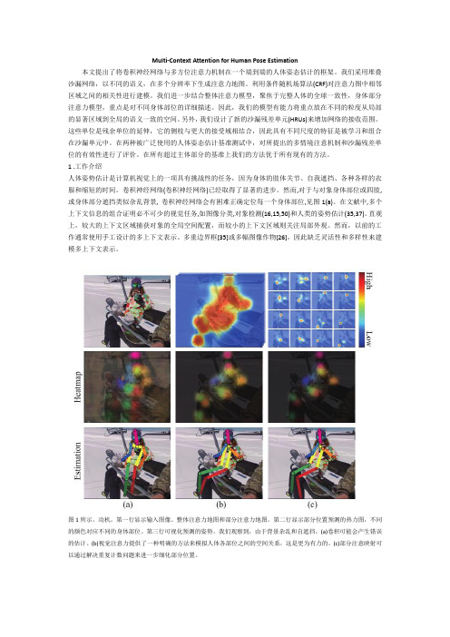
Multi-Context Attention for Human Pose Estimation本文提出了将卷积神经网络与多方位注意力机制在一个端到端的人体姿态估计的框架。

我们采用堆叠沙漏网络，以不同的语义，在多个分辨率下生成注意力地图。

利用条件随机场算法(CRF)对注意力图中相邻区域之间的相关性进行建模。

我们进一步结合整体注意力模型，聚焦于完整人体的全球一致性，身体部分注意力模型，重点是对不同身体部位的详细描述。

因此，我们的模型有能力将重点放在不同的粒度从局部的显著区域到全局的语义一致的空间。

另外，我们设计了新的沙漏残差单元(HRUs)来增加网络的接收范围。

这些单位是残余单位的延伸，它的侧枝与更大的接受域相结合，因此具有不同尺度的特征是被学习和组合在沙漏单元中。

在两种被广泛使用的人体姿态估计基准测试中，对所提出的多情境注意机制和沙漏残差单位的有效性进行了评价。

在所有超过主体部分的基准上我们的方法优于所有现有的方法。

1 .工作介绍人体姿势估计是计算机视觉上的一项具有挑战性的任务，因为身体的肢体关节、自我遮挡、各种各样的衣服和缩短的时间。

卷积神经网络(卷积神经网络)已经取得了显著的进步。

然而,对于与对象身体部位或四肢,或身体部分遮挡类似杂乱背景, 卷积神经网络会有困难正确定位每一个身体部位,见图1(a)。

在文献中,多个上下文信息的组合证明必不可少的视觉任务,如图像分类,对象检测(16,15,50)和人类的姿势估计(35,37)。

直观上，较大的上下文区域捕获对象的全局空间配置，而较小的上下文区域则关注局部外观。

然而，以前的工作通常使用手工设计的多上下文表示。

多重边界框[35]或多幅图像作物[26]，因此缺乏灵活性和多样性来建模多上下文表示。

图1所示。

动机。

第一行显示输入图像、整体注意力地图和部分注意力地图。

第二行显示部分位置预测的热力图，不同的颜色对应不同的身体部位。

第三行可视化预测的姿势。

我们观察到，由于背景杂乱和自遮挡，(a)卷积可能会产生错误的估计。

Author QueriesJOB NUMBER:MS213840JOURNAL:GPAAQ1We have inserted a running head.Please approve or provide an alternative.Q2Please supply received,revised and accepted dates.Counting people using video camerasDAMIAN ROQUEIRO†*and V ALERY A.PETRUSHIN‡{†Department of Computer Science,University of Illinois at Chicago,Chicago,IL 60607,USA‡Accenture Technology Labs,Chicago,IL 60601,USA(Received B ;revised B ;in final form B )Q2The paper is devoted to the problem of estimating the number of people visible in a camera.It uses as features the ratio of foreground pixels in each cell of a rectangular ing the above features and data mining techniques allowed reaching accuracy up to 85%for exact match and up to 95%for plus–minus one estimates for an indoor surveillance environment.Applying median filters to the sequence of estimation results increased the accuracy up to 91%for exact match.The architecture of a real-time people counting estimator is suggested.The results of analysis of experimental data are provided and discussed.Keywords :Multi-camera surveillance;Video surveillance;Counting people;Machine learning algorithms;Number of people estimation1.IntroductionCounting people is an important task in automatic surveillance systems.It can serve as a subtask in multiple stage processing or can be of primary interest.The robust estimate of people count could improve low level procedures,such as blob extraction or it can provide answers to questions such as,how many people were inside the room between time stamps t 1and t 2?The related problem is to estimate the density of people in a crowd in places such as a subway platform or a ually the output is a “fill rate”of the space expressed as a percentage.To solve this problem,different types of location sensors could be used.We will not attempt to exhaustively enumerate all the types of location sensors (see Ref.[1]for a survey).However,we can mention some special sensors that are used mostly in indoor environments and for which there are many commercial solutions already in place:electro-optical,thermic and passive-optics directional sensors are just a few.These sensors are placed in the entrances of buildings,rooms or vehicles.They can detect the passage and direction of a person and report with high accuracy the count of people that entered or left the facility,but they come atThe International Journal of Parallel,Emergent and Distributed Systems ISSN 1744-5760print/ISSN 1744-5779online q 2006Taylor &Francis/journals DOI:10.1080/17445760601139096*Corresponding author.Email:droque1@ {Email:valery.a.petrushin@GPAA 213840—8/12/2006—SWAPNA—245462The International Journal of Parallel,Emergent and Distributed Systems ,Vol.00,No.0,2006,1–1751015202530354045the cost of having to install proprietary hardware (the sensors and the data collection devices)and software to analyse the data.In contrast to this,video-based sensors—or video cameras—have increasingly become a commercial off-the-shelf product for surveillance purposes.Additionally,existing video cameras used for surveillance can be leveraged to perform more tasks such as automatic tracking,behaviour recognition and crowd estimation,among others.2.Related workIn the past years there has been a bulk of research work in the area of image processing with the objective of obtaining more accurate and reliable people-count estimations.An intuitive solution to the problem of estimating the size of a crowd in an image will be,literally,to obtain a head count.While this would be a tedious,but yet feasible,task for a human it certainly is a difficult problem for an automatic system.That is exactly the problem tackled in Ref.[2],where wavelets are used to extract head-shaped features from the image.Further processing uses a support vector machine to correctly classify the feature as a “head”or “something else”and applies a perspective transform to account for the distance to the camera.A similar idea is used in Ref.[3],where a face detection program is used to determine the person count.Unfortunately,as pointed out by its authors,this method is affected by the angle of view at which the faces are exposed to the camera.Additionally,images where a person’s back is only visible will result in a poor estimation as well.Another approach has been suggested in Ref.[4],it aims to obtain an estimation of the crowd density,not the exact number of people.It requires a reference image—where no people are present,in order to determine the foreground pixels in a new image.A single layer neural network is fed with the features extracted from the new image (edge count and densities of the background and crowd objects)and the hybrid global learning algorithm is used to obtain a refined estimation of the crowd density.Our work compares different classification algorithms for estimating the number of people in an image obtained from a video surveillance camera.This approach differs from previous works in that we do not attempt to obtain and count specific features from the images (head-shaped objects in Ref.[2]or faces in Ref.[3]).We just exploit the correlation between the percentage of foreground pixels and the number of people in an image [5].3.DatasetsIn order to determine how different classification algorithms would perform on both an outdoor environment with high traffic and an indoor environment with moderate and low traffic,we selected the following two sources:(1)a publicly available webcam at Times Square;and (2)two webcams in the premises of the Accenture Technology Labs in Chicago.The Times Square webcam,denoted herein as camTS ,is located at the intersection of 46th Street and Broadway in New York City and it streams video images through a publicly available URL [6].In contrast,the remaining two webcams can only be accessed from within the Accenture intranet and are part of a larger set of webcams of an experimental surveillanceGPAA 213840—8/12/2006—SWAPNA—245462D.Roqueiro and V .A.Petrushin2505560657075808590system already in place.The two cameras chosen for the experiments have opposite views of an elevator area on the 36th floor.This area is the gateway to the offices of the Accenture Q1Technology Labs located on the same floor,and the cameras will be referred as camEE and camEW ,covering the elevators from the East and West,respectively.The three cameras capture snapshot images in the JPEG format but with different resolutions:353£239for camTS and 640£480for camEE and camEW .3.1Image pre-processingThe features we extracted from the images were based on the density of foreground pixels.To extract the foreground pixels we used the well known median filter background modelling technique [7].According to this technique each background pixel is modelled as median of a pool of images accumulated over some period of time and periodically updated by adding the current image and discarding the oldest one.This technique works well when each background pixel is occluded in less than 50%of images of the pool.To get the foreground pixels the background model is subtracted from the current image pixel by pixel,the absolute values of differences are summed and compared to a threshold.All pixels that have a difference above the threshold are marked as foreground.Then morphological operations are applied to smooth the result.Figure 1(b),(d)show the binary images with the results of foreground pixel extraction.The original images (figure 1(a),(b))have an ignore-zonethatFigure 1.Captured images from the three webcams and their respective binary images with foreground pixels (the ignore zones and grids are shown for illustrational purposes only);(a)camTS captured image;ignore zone above y ¼60;(b)camTS binary image with foreground pixels;original grid of 83cells;size of each cell is 25£30pixels;(c)camEE captured image;ignore zone above y ¼40;(d)camEE binary image with foreground pixels;grid of 176cells of 40£40pixels.GPAA 213840—8/12/2006—SWAPNA—245462Counting people using video cameras395100105110115120125130135represents an area of the image not worth using and from which no features are extracted.There was no ignore-zone defined for camEW .3.2Feature extractionFor each camera,we created three grids of different size and applied them to the binary images to obtain three datasets.A record of a dataset has the image ID and N real values in the range from 0to 1,which correspond to the portion of foreground pixels in each cell (count of foreground pixels in the cell divided by its area).The size of the cells is arbitrary and for our experiments we considered grid sizes that differ by a factor of two:double (2x)or half the size (0.5x)of the original (1x).For camTS the original cell size was of 25£30pixels whereas for camEE and camEW it was 40£40.We wanted to learn how the sizes of the cells influenced the accuracy of the classification algorithms.Figure 1shows the sample layouts for two of the cameras that have been used in the experiments.3.3LabellingThe images from camTS were collected in the spring of 2005during several days between 10:00am and 3:00pm.The images for the other two webcams were recorded on 6different days,between 11:50am and 2:00pm,to benefit from the “rush-hour”activity at lunch time.They were captured at a frame rate that varied from 2to 9images/s and they were not synchronized (camEE could have captured one image in 1s while camEW captured four in the same period).This raw set of images was analysed and several hundreds of them had to be discarded due to flickering in the cameras.Once the final set of images was clearly defined,we manually labelled them associating to each image the number of people visible in it.Even if part of a person was visible,it was still counted.The count was added as another attribute to the existing records in the datasets.Figure 2(a)–(c)show the distribution of ground truth counts of people for the three original datasets.The original data contain 1452images for camTS ,17,604images for camEE and 26,718images for camEW .As it can be seen from the two distributions in figure 2(b),(c),the datasets for the webcams covering the elevator area were biased toward low number of people.To improve the performance of the classification algorithms we decided to create two reduced datasets that have a more uniform distribution for low number of people.These datasets have a total of 3565images for camEE and 4974images for camEW ,and their records were randomly selected from the original datasets.The distribution of labels in the reduced datasets is presented in figure 2(d),(e).4.Classification algorithmsThis section lists the algorithms used in our experiments and their parameters.For the sake of clarity,we would like to briefly explain how the algorithms were tested and what data they used.This digression will help the reader to understand how the datasets were actually processed.Each image that was captured and processed will have a matching record in a dataset with:a label and N values.The label is the count of persons in the image and the N values are the proportion of foreground pixels in each cell of the N -grid.For a givenGPAA 213840—8/12/2006—SWAPNA—245462D.Roqueiro and V .A.Petrushin4140145150155160165170175180classification method,some records from the dataset are used to train it.The rest of the records are used to test it and the labels are compared to the predicted values.This gives us a measure of the accuracy of the algorithm to estimate the count of persons in unseen images from the test set.4.1Algorithms implementedWe implemented the following algorithms:(a)multiple linear regression ;(b)k-nearest neighbour with Euclidean distance;(c)a two-layer resilient backpropagation neural network (BPNN)with a log-sigmoid transfer function for the first layer and ten neurons [8,9].The second layer has a linear transfer function and its output was rounded to the closest integer number;(d)a two-layer probabilistic neural network (PNN)[10].The first layer is a radial basis layer that computes the distance (probability)of a new vector to the training input vectors and then a competitive layer finds the maximum of these probabilities;and (e)support vector machines (SVM)5.ResultsThe methodology implemented to compare the above mentioned classifiers follows the traditional sequence of steps used in creating and evaluating supervised learning algorithms.Each classifier was trained and tested with different datasets and,unless otherwise noted,all the experiments detailed in this section were repeated 100times to attain statisticalDistribution of labels for camTSPersonsN u m b e r o f c a s e sOriginal distribution of labels for camEEPersonsPersonsN u m b e r o f ca s e sOriginal distribution of labels for camEWPersonsReduced distribution of labels for camEEN u m b e r o f c a s e sReduced distribution of labels for camEWPersons(a)(b)(d)(e)(c)Figure 2.Distribution of labels for the original and reduced datasets.GPAA 213840—8/12/2006—SWAPNA—245462Counting people using video cameras5185190195200205210215220225significance.At each iteration,70%of the records of the dataset were randomly selected to train the classifier and the remaining 30%was used to test it.Then the labels in the test set were compared to the output generated by the classifier and the accuracy of the classifier was estimated.The records in the training and test set were randomly selected using a uniform distribution.Before an experiment started,all the records in the dataset were shuffled to avoid any side effects due to the chronological order of the images§.The experiments were run using Matlab w 7.1on a Pentium 4,2.8GHz CPU with 512Mb of RAM.Two-third party toolboxes were used for SVM [11]and k -nearest neighbour [12].Before presenting the results of our experiments,we would like to revisit the goal of this work.Our original goal of finding a method to estimate the count of people in an image can be refined further as two sub-goals:(1)Find a classifier to determine with certain reliability if there are zero-persons in animage.(2)Find a classifier to estimate the count of people in an image that has one or more people.In some real settings it makes sense first to filter out frames when no people are present in front of a camera.This two-step process can both expedite the recognition process and improve the accuracy of the person count estimation.An architecture that will implement this idea is depicted in figure 3.First,an image is captured and pre-processed to obtain the foreground pixels.Based on a given grid,the percentage of foreground pixels in each cell of the grid is determined.These values are then used by an already trained classification algorithm that determines if the number of people in the image is zero (zero-person detector).If the image is classified as having zero people,it is discarded.Otherwise another classifier is used to estimate the people count and the whole process is repeated for a new image.This section describes our experience for finding the best classifier for each of the above mentioned sub-goals.For zero-person detection we tested k -nearest neighbour,the PNN and SVM with the 1x grid.For counting people we tested all the classifiers,except for SVM,with the three grid sizes (1x,2x and 0.5x).5.1Zero-person detectionHere we tackle the problem of creating a recogniser that classifies images into two classes,when (a)no person;and (b)one or more persons are visible in the image.Taking into account that a simple threshold applied to the percentage of foreground pixels does not work well (for example,when the elevator doors opened or closed and no people were visible),we decided to use machine learning techniques to solve the problem.We evaluated three different classifiers for this task:(1)SVM,(2)k -nearest neighbour with k ¼1;and (3)a PNN.The classifiers were tested using the original datasets described in Section 3.3,where all labels with values 1or more were substituted with value 1.§As it will become clear in Section 6,training the classifiers with shuffled data provides us with a baseline for accuracy that leaves room for improvement,e.g.if the classifier can take advantage of the chronological order of the images.GPAA 213840—8/12/2006—SWAPNA—245462D.Roqueiro and V .A.Petrushin6230235240245250255260265270Our results show that SVM was slightly more accurate than the other classifiers in two datasets (camTS and camEE )while having a comparable accuracy to k -nearest neighbour for camEW .In general,SVM and k -nearest neighbour were significantly more accurate than the probabilistic neural network.Table 1shows the confusion matrices obtained for camEE .To obtain the execution times,we had to perform two different time measurements:one at the group level—measure the time to train 70%of the dataset and to classify the remaining 30%and one at the individual record level.Although high accuracy is very desirable,it cannot come at the price of a slow performance.In that aspect,table 2shows how k -nearest neighbour outperforms SVM by a factor of 10.Clearly,from the values in table 2,we cannot take the time required by a method to classify 1070records and divide it by 1070to obtain the time to classify one record.That is why the average execution time of classifying only one record had to be computed separately.From an implementation perspective these functions have an overhead that cannot be ignored,especially since we target to do classification in real-time.5.2Counting peopleAs it was mentioned before,if an image is classified as having one or more persons in it we proceed to run a classifier that will estimate the people count in the image.This means that,when comparing the classification algorithms,we can assume that the datasets have no records with labels equal to zero.To do so,we used the reduced datasets described in Section 3.3and deleted the records with images that were labelled as havingzero-persons.Figure 3.Architecture of a real-time person counter.Table 1.Confusion matrices with results of classification between 0or 1þpersons (one or more)for camEE andgrid size 1x.SVM 1-nearest neighbourPNN Predicted Predicted Predicted1þ01þ01þActual 096.49 3.5197.56 2.44100.000.001þ0.6099.40 1.1498.86 4.0995.91Total Accuracy98.86%98.64%96.61%GPAA 213840—8/12/2006—SWAPNA—245462Counting people using video cameras7275280285290295300305310315These “reduced-no-zeros”datasets have 1442,2960and 4121records for camTS ,camEE and camEW ,respectively.The following classification methods were evaluated:(1)Multiple Linear Regression;(2)Regression Tree;(3)k -nearest neighbour;(4)Backpropagation neural network (BPNN);and (5)Probabilistic neural network (PNN).Once the results were obtained,the methods were compared according to three variables of interest:(a)accuracy;(b)training time;and (c)execution time.Accuracy .The accuracy of a method was categorized in four levels:the first,and most desirable one,is exact match.This level has the percentage of accurate estimations,i.e.when the classifier—for a given image—reported a person count that was equal to the label assigned to that image.The other three levels account for the estimations that had a difference of 1person (þ1or 21),2(þ2,22)and 3(þ3,23)persons,respectively.The accuracy is reported in a cumulative fashion,for example,the percentage of estimations with a difference of 2includes the exact matches and the estimations that were off by 1.Training time .This time has different implications according to the classification method analysed.For Multiple Linear Regression,the training time is the time required to solve the system of equations.In the case of a Regression Tree,it is not only the time necessary to create the tree but also to prune it.k -nearest neighbour does not have a training phase and for both neural networks,the training time has the correct interpretation.In all cases,this time is expressed in seconds and involved the processing of 70%of the dataset in question.Execution time .It is the time required for a classifier to classify only one record.It will also be expressed in seconds and,in the case of very small numbers,in scientific notation.Table 3shows the accuracy of the classifiers for exact match.At first sight,Linear Regression and Regression Tree do not seem to be good classifiers.If instead of focusing on exact matches we consider a difference of 3(þ3or 23)the mean accuracy for this two classifiers can in some cases be above 95%and as close as to 100%.Of course,this relaxation in our prediction can be acceptable in an environment similar to the one covered by the Times Square webcam.In this case,when having to determine the count of people in a crowd of 20Table parison of execution times between classifiers for camEE .Number of recordsMean time (in seconds)SVM1-nearest neighbourPNN Train 2495(70%)68.94N/A 0.20Classify1070(30%)7.0925.4632.72One record0.260.020.05Table 3.Mean accuracy (in percentage)for exact match.Dataset methodcamTS camEE camEW 1x2x 0.5x 1x 2x 0.5x 1x 2x 0.5x Multiple linear regression 21.720.022.547.948.644.656.950.558.4Regression tree 22.721.322.269.669.768.371.972.970.41-nearest neighbour 36.537.036.983.379.685.086.685.586.9BPNN 27.321.531.265.759.767.069.965.069.5PNN37.037.030.583.072.980.786.283.579.8GPAA 213840—8/12/2006—SWAPNA—245462D.Roqueiro and V .A.Petrushin8320325330335340345350355360persons,an estimation of 23may be acceptable.On the other hand,in a confined and controlled area as the one covered by camEE and camEW ,we would expect a higher accuracy for exact matches and will probably consider a difference of up to 1.For this,1-nearest neighbour,the BPNN and the PNN provide a better estimation.The k -nearest neighbour classifier was evaluated for different values of k ¼1,3,5and 7and the best results were obtained when k ¼1;with the mean accuracy degrading for higher values of k .For example,for camEE (dataset 1x)and k ¼3;5and 7the mean accuracy for exact match was 80,77.6and 76.3%,respectively.It is worth mentioning that the density of the grid has an effect on k -nearest neighbour.For the webcams in the elevator area we had a higher accuracy when the density of the grid increased (the size of the cells decreased).As an example,for camEE and grids of 1x,2x and 0.5x the accuracies of up to a difference of 1were 95.9,94.5and 96.4%.It is just a slight increase in accuracy but,as we could have expected,the classifier takes advantage of the extra number of features to find a better match.The BPNN does not provide a high accuracy for exact matches but improves dramatically when considering a difference of 1.In particular,for camEE and camEW the precision increases at least to 95%.The PNN outperforms the BPNN in exact matches for all datasets and grid sizes—except for camTS and grid 0.5x—but has a comparable performance with BPNN when considering a difference of 1.Also of interest,is the fact that the number of cells in the grid does not improve the classification for PNN.Considering the mean accuracy of these methods,1-nearest neighbour and PNN provide equivalent results.Figure 4compares the mean accuracy for exact matches in the original grid (1x)for all three webcams.Figures 5and 6illustrate the mean accuracy for the different labels.In the case of camTS (figure 5),1-nearest neighbour gives slightly better estimations for exact matches.For the other webcams (figure 6(a),(b)),as it was mentioned before,the mean accuracy of the PNN is comparable to that of the BPNN when considering a difference of 1.The training and execution time were also calculated for each classifier.In practice,the training time is not important in determining the most appropriate classifier because training is conducted off-line.Therefore,we put more stress on comparing the methods based on their execution time,i.e.the time it takes the classifier to estimate the number of people in one image.Table 4lists the execution times of the classifiers for the different datasets.Due to their architecture the PNNs have shorter training time and larger execution time in comparison to the BPNN,which in turn is computationally more expensive to train,but faster to execute.The execution of multiple linear regression is just a dot product of twovectors,Figure parison of mean accuracy (exact match)for three cameras.GPAA 213840—8/12/2006—SWAPNA—245462Counting people using video cameras9365370375380385390395400405thus it has extremely fast execution time.The execution time of a nearest neighbour approach depends on the number of cells and size of the dataset.6.ExtensionsThe results presented in the previous section provide a foundation for creating a real-time person counter as the one depicted in figure 3with two main modules:(a)a zero-person classifier;and (b)a counting-people estimator.We can pick up a pair of classifiers that gives the best accuracy,but the total accuracy depends on how well the counting-people estimator treats the situation when it is fed with wrong output from the zero-person classifier.In general we have three sources of error,namely:(1)An image with no persons is classified as 1þby the zero-person classifier.(2)An image with 1þpersons is classified as 0by the zero-person classifier.(3)An image with 1þpersons is classified as 1þby the zero-person classifier but thefinal count is incorrectly estimated by the counting-people classifier.When the percentage of errors from 1to 2are sufficiently close to zero,the accuracy of the whole system—for exact match—will be close to what was shown in table 3(note that the third source of error listed before is the complement of the figures in table 3).We know from table 1that,for camEE ,we can expect SVM and 1-nearest neighbour to produce 1.14and 1.36%of errors 1and 2combined,respectively.This section addresses these problems and attemptstoFigure 5.Results for 1-nearest neighbor (camTS1x).Figure 6.Mean accuracy for camEE (1x);using (a)PNN and for (b)BPNN.GPAA 213840—8/12/2006—SWAPNA—245462D.Roqueiro and V .A.Petrushin10410415420425430435440445450simulate (off-line)a real-time person counter.Our goal is to extend our analysis and to explore techniques that could help the real-time person counter to increase its accuracy and minimize the effect of the errors in the predictions of 0or 1þpersons for the elevator cameras camEE and camEW .The strategies we will explore include:(1)utilization of median filters;(2)creation of an assorted (heterogeneous)grid;and (3)variable (feature)selection.6.1Median filtersA median filter with window of size k (where k is an odd number)scans a sequence of numbers and replaces a value in the middle position with the median value of the window.The advantage of the median filters is that they can smooth the result without averaging the values.Applying median filters to a sequence of chronologically ordered images that were captured within a certain time interval,we can correct the output of our classifiers.Let us assume that a counting-people classifier predicted the sequence of counts depicted in figure 7(a).If the time interval between the images is not large,we would expect a smooth transition of counters.As a result of this,we can notice that number 8in the 5th position is an incorrect prediction due to,probably,flickering of the camera,and the value 1in the 15th position is likely the result of occlusion of a person by another ing a median filter with a window of size 3corrects the errors (figure 7(b)).The real-time person counter can use a median filter to correct the results of the zero-person classifier,the counting-people estimator or ing a median filter introduces a delay,which depends on the frame rate of the camera and the filter’s window size.For majority of applications a delay of 1–3s could be acceptable when it brings a benefit of increasing accuracy by 3–5%.We assume that the output of the zero-person classifier will be corrected with a median filter before invoking the counting-people classifier for those images classified as 1þ,and another median filter will be applied to the results to create the final estimations.At every point,if the interval between images is larger than a threshold then theTable 4.Average execution time in seconds.Dataset methodcamTSCamEEcamEW1x2x 0.5x 1x 2x 0.5x 1x 2x 0.5x Multiple linear regression 1.e-5 1.e-5 1.e-5 2.e-5 1.e-5 2.e-5 2.e-5 1.e-5 4.e-5Regression tree 8.e-47.e-48.e-40.0020.0010.0010.0019.e-40.0061-nearest neighbour 0.0050.0010.0100.0200.0060.0840.0310.0090.122BPNN 0.0050.0050.0050.0060.0050.0060.0050.0050.005PNN0.0150.0070.0230.0450.0170.1600.0610.0210.224Figure 7.A sample sequence of counts with (a)two errors and (b)the corrected sequence after a median filter with window size ws ¼3was applied.GPAA 213840—8/12/2006—SWAPNA—245462Counting people using video cameras 11455460465470475480485490495。

CVPR 2013 录用论文（目标跟踪部分）/gxf1027/article/details/8650878完整录用论文官方链接：/cvpr13/program.php过段时间CvPaper上面应该会有正文链接今年有关RGB-D摄像机应用和研究的论文渐多起来了。

当然，自己还是比较关心Tracking方面的Papers。

从作者来看，一作大部分为华人，而且有不少在Tracking这个圈子里相当有名的牛，比如Ming-Hsuan Yang，Robert Collins等（中科院到阿大的Xi Li也是非常活跃，从他的论文可以看出深厚的数学功底，另外Chunhua Shen老师团队非常高产）。

此外，从录用论文题目初步判断，Sparse coding （representation）的热度在减退，所以Haibin Ling老师并没有这方面的文章录用，且纯粹的tracking-by-detection几乎不见踪影了。

以下是摘录的tracking方面的录用论文：Oral部分：Structure Preserving Object Tracking. Lu Zhang, Laurens van der MaatenTracking Sports Players with Context-Conditioned Motion Models. Jingchen Liu, Peter Carr, Robert Collins, Yanxi Liu Post部分：Online Object Tracking: A Benchmark. Yi Wu, Jongwoo Lim,Ming-Hsuan YangLearning Compact Binary Codes for Visual Tracking. Xi Li, Chunhua Shen, Anthony Dick, Anton van den HengelPart-based Visual Tracking with Online Latent Structural Learning. Rui Yao, Qinfeng Shi,Chunhua Shen, Yanning Zhang, Anton van den HengelSelf-paced learning for long-term tracking.James Supancic III, Deva Ramanan（long-term的噱头还是很吸引人的，和当年TLD一样，看看是否是工程的思想多一些）Visual Tracking via Locality Sensitive Histograms.Shengfeng He, Qingxiong Yang, Rynson Lau, Jiang Wang,Ming-Hsuan Yang （CityU of HK，使用直方图作为表观在当前研究背景下真是反其道而行之啊）Minimum Uncertainty Gap for Robust Visual Tracking. Junseok Kwon, Kyoung Mu Lee （VTD作者）Least Soft-thresold Squares Tracking. Dong Wang, Huchuan Lu, Ming-Hsuan YangTracking People and Their Objects. Tobias Baumgartner, Dennis Mitzel, Bastian Leibe（这个应该也有应用的背景和前景）（以上不全包括多目标跟踪方面的论文）其它关注的论文：Alternating Decision Forests. Samuel Schulter, Paul Wohlhart,Christian Leistner, Amir Saffari,Peter M. Roth,Horst Bischof（Forest也是近些年的热点之一。

openpose的相关文献以下是一些与OpenPose相关的文献：1. Cao, Z., Simon, T., Wei, S. E., & Sheikh, Y. (2017). Realtime multi-person 2D pose estimation using part affinity fields. In Proceedings of the IEEE Conference on Computer Vision and Pattern Recognition (pp. 7291-7299). 这是OpenPose的原始论文，介绍了OpenPose方法的细节和实现。

2. Simon, T., Joo, H., Matthews, I., & Sheikh, Y. (2017). Hand keypoint detection in single images using multiview bootstrapping. In Proceedings of the IEEE Conference on Computer Vision and Pattern Recognition (pp. 4645-4653). 这篇论文介绍了OpenPose中关于手部关键点检测的方法。

3. Cao, Z., Hidalgo Martinez, G., & Simon, T. (2018). OpenPose: realtime multi-person 2D pose estimation using part affinity fields (arXiv preprint arXiv:1812.08008). 这是OpenPose方法的更新版本，介绍了一些改进和优化。

4. Guler, R. A., & Koksal, M. S. (2018). Densepose: Dense human pose estimation in the wild. In Proceedings of the IEEE Conference on Computer Vision and Pattern Recognition (pp. 7297-7306). 这篇论文介绍了DensePose，一种与OpenPose类似的密集姿态估计方法。

二维人体姿态估计研究综述李崤河; 刘进锋【期刊名称】《《现代计算机（专业版）》》【年(卷),期】2019(000)022【总页数】5页(P33-37)【关键词】深度学习; 人体姿态估计; 关键点检测【作者】李崤河; 刘进锋【作者单位】宁夏大学信息工程学院银川750021【正文语种】中文0 引言人体姿态估计长久以来一直是计算机视觉领域的一个热点问题。

其主要内容，是让计算机从图像或视频中定位出人物的关键点（也称为关节点，如肘、手腕等）。

人体姿态估计作为理解图像或视频中人物动作的基础，一直受到众多学者的关注。

随着计算机技术的迅猛发展，人体姿态估计已经在动作识别、人机交互、智能安防、增强现实等领域获得了广泛应用。

人体姿态估计按维度可分为二维和三维两种：二维人体姿态估计通常使用线段或者矩形来描述人体各关节在图像上的投影位置，线段的长度和角度表示了人体的二维姿态；三维人体姿态估计通常使用树模型来描述估计的姿态，各关节点的位置使用三维坐标确定。

在实际应用中，目前获取的大多数图像仍是二维图像，同时三维姿态估计可以使用二维预测进行推理[1]，所以二维姿态估计有着重要的研究价值。

自人体姿态估计的概念提出以来，国内外的学者对此做出了不懈的努力。

传统的姿态估计算法主要是基于图结构（Pictorial Structures）模型[2]。

该模型将人或物体表示为多个部件的集合，这些部件之间含有空间约束，通过人工指定的特征检测组件实现关节点检测。

传统方法过于依赖手工设计的模板，难以应付复杂的姿态变换并且推广到多人姿态估计。

随着深度学习技术在计算机视觉领域大放异彩，部分学者开始研究如何利用深度学习来解决人体姿态估计问题。

Toshev 等人利用深度卷积神经网络对人体姿态进行全局推断，提出了完全基于神经网络的模型DeepPose[3]。

DeepPose 是第一个将深度学习方法应用于人体姿态估计的主要模型。

该模型实现了SOTA 性能并击败了当时的传统模型。

Shape-From-Silhouette of Articulated Objects and its Use for Human Body Kinematics Estimation and Motion Capture German K.M.Cheung Simon Baker Takeo KanadeRobotics Institute,Carnegie Mellon University,Pittsburgh PA15213german+@ simonb+@ tk+@AbstractShape-From-Silhouette(SFS),also known as Visual Hull (VH)construction,is a popular3D reconstruction method which estimates the shape of an object from multiple silhou-ette images.The original SFS formulation assumes that all of the silhouette images are captured either at the same time or while the object is static.This assumption is violated when the object moves or changes shape.Hence the use of SFS with moving objects has been restricted to treating each time instant sequentially and independently.Recently we have successfully extended the traditional SFS formu-lation to refine the shape of a rigidly moving object over time.Here we further extend SFS to apply to dynamic ar-ticulated objects.Given silhouettes of a moving articulated object,the process of recovering the shape and motion re-quires two steps:(1)correctly segmenting(points on the boundary of)the silhouettes to each articulated part of the object,(2)estimating the motion of each individual part us-ing the segmented silhouette.In this paper,we propose an iterative algorithm to solve this simultaneous assignment and alignment problem.Once we have estimated the shape and motion of each part of the object,the articulation points between each pair of rigid parts are obtained by solving a simple motion constraint between the connected parts.To validate our algorithm,wefirst apply it to segment the dif-ferent body parts and estimate the joint positions of a per-son.The acquired kinematic(shape and joint)information is then used to track the motion of the person in new video sequences.1.IntroductionTraditional Shape-From-Silhouette(SFS)assumes either that all of the silhouette images are captured at the same time or that the object is static[15,18,14].Although sys-tems have been proposed to apply SFS to video[5,2],these systems apply SFS to each frame sequentially and inde-pendently.Recently there has been some work on using SFS on rigidly moving objects to recover shape and motion [21,22],or to refine the shape over time[4].These meth-ods involve the estimation of the6DOF rigid motion of the object between successive frames.In[22]the motion is as-sumed to be circular.Frontier points are extracted from the silhouette boundary and used to estimate the axis of rota-tion.In[21],Ponce et al.define a local parabolic structure on the surface of a smooth curved object and use epipolar geometry to locate corresponding frontier points on three silhouette images.The motion between the images is then estimated by a two-step minimization.In[4]the6DOF motion is estimated by combining both the silhouette and the color information.At each time in-stant,3D line segments called Bounding Edges are con-structed from rays through the camera centers and points on the silhouette ing the fact that each Bounding Edge touches the object at at least one point,a multi-view stereo algorithm is proposed to extract the colors and posi-tions of these touching points(subsequently referred to as Colored Surface Points).The motion between consecutive frames is then computed by minimizing the errors of pro-jecting the Colored Surface Points into the images.Once the6DOF rigid motion is recovered and compensated for, all the silhouette images are treated as taken at the same time and traditional SFS is applied to get a refined shape of the object.In this paper we extend[4]to handle articulated objects. An articulated object consists of a set of rigidly moving parts which are connected to each other at certain articu-lation points.A good example of an articulated object is the human body(if we approximate the body parts as rigid). Here we propose an algorithm to automatically recover the joint positions,and the shape and motion of each part of an articulated object.We begin with silhouette images,al-though color information is used to break the alignment am-biguity as in[4].Given silhouettes of a moving articulated object,recov-ering the shape and motion requires two inter-related steps: (1)correctly segment(points on the boundary of)the silhou-ettes to each part of the object and(2)estimate the shape and motion of the individual parts.We propose an itera-tive algorithm to solve this simultaneous assignment and 6DOF motion estimation problem.Once the motions of the rigid parts are known,their articulation points are es-timated by imposing motion constraints between adjoining parts.To test our algorithm,we apply it to acquire the shape and joint locations of articulated human models.Once this kinematic information of the person has been acquired,we show how the6DOF motion estimation algorithm can be used to track the articulated motion of that person in new video sequences.Results on both synthetic and real data are presented to show the validity of our algorithms.Bounding EdgeCamera center 3Object Oi r 1E 1 i& I13Figure1.The Bounding Edge is obtained byfirst pro-jecting the ray onto,,and then re-projecting thesegments overlapping the silhouettes back into3D space.is the intersection of the reprojected segments.The point where the object touches is located by searchingalong for the point with the minimum projected colorvariance.Note that the image from camera4is not usedbecause it is occluded.See[4]for details.2.BackgroundIn[3]and[4]we extended the traditional SFS formu-lation to rigidly moving bining the silhouette and color images,wefirst extract3D points on the surface of the object at each time instant.These surface points are then used to estimate the6DOF motion between succes-sive frames.Once the rigid motion across time is known, all of the silhouette images are treated as being captured at the same time and SFS is performed to estimate the shape of the object.Below we give a brief review of this temporal SFS algorithm.2.1.Visual Hulls and Their Bounding EdgesThe term Visual Hull(VH)wasfirst coined by Lauren-tini in[13]to denote the3D shape obtained by intersecting the visual cones formed by the silhouette images and the camera centers[13,14,2].One useful property of a VH is that it provides an upper bound on the shape of the ob-ject.In[4],we introduced a new representation of a VH called the Bounding Edge representation.Assume there are color-balanced and calibrated cameras positioned around a Lambertian object.Letbe the set of color and corresponding silhouette images of the object obtained from the cameras at time.Let be a point on the boundary of the silhouette image. Through the center of camera,defines a ray in3D space.A Bounding Edge is defined as the portion of such that the projection of on the image planes of all the other cameras lies completely inside the silhouettes.An example is shown in Figure1.can be constructed by successively projecting the ray onto each silhouette im-age,and retaining the portion whose projection overlaps all the silhouettes.2.2.Colored Surface Points(CSP)The most important property of a Bounding Edge is the Second Fundamental Property of Visual Hulls(2nd FPVH) which states that each Bounding Edge touches the object (which forms the silhouette images)at at least one point [4].Using this property,we are able to locate points on the surface of the object using a multi-stereo color match-ing approach.Consider a Bounding Edge.Since we assume the object is Lambertian and the cameras are color balanced,there exists at least one point on(the point where it touches the object)such that the projected colors of this point in all the visible color images are the same. In other words,this point has zero projected color variance among the visible color images.In practice,due to noise and inaccuracies in color balancing,instead of searching for the point that has zero projected color variance,we assign the touching point on to be the point with the minimum color variance,as shown in Figure1.We refer to this point as a Colored Surface Point(CSP)of the object and repre-sent its position and color(which is obtained by averaging its projected color across all visible cameras)by and respectively.By sampling the boundaries of all the sil-houette images,a set of Colored Surface Points can be constructed.Note that there is no point-to-point correspon-dence relationship between two different sets of CSPs ob-tained at different time instant.The only property common to the CSPs is that they all lie on the surface of the object.2.3.SFS Across Time for Rigid ObjectsWe now describe our algorithm for recovering the6DOF motion of a rigid object using the CSPs.Without loss of generality,we assume that the orientation and position of the object at time is0¯and that at time it is.The rigid object alignment prob-lem is then equivalent to recovering.Consider the motion between and as an example and assume we have two sets of dataobtained at and respectively. Tofind,we align the CSPs with the2D silhouette and color images.The idea is very similar to that in[19]for 2D image alignment.Suppose we have an estimate of.For a CSP (with color)at time,its3D position at time would be.Consider two different cases of the projection of into the camera:1.The projection lies inside the silhouette.In thiscase,we use the color difference as an error measure:(1)where is the projected color of a3D pointinto the color image.Here we assume this color error is zero if the projection of lies outside.(b)(a)(d)(c)Figure 2.Results of our temporal SFS algorithm [4]applied to synthetic data:(a)one of the input images,(b)unaligned CSPs,(c)aligned CSPs,(d)refined visual hull.2.The projection lies outside.In this case,we use the distance of the projection from ,represented byas an error measure.The distance iszero if the projection lies inside .Summing over all cameras in which is visible,the errormeasure of with respect tois given by(2)where is a weighing constant.Similarly,the error measure of a CSP at time is written as(3)Now the problem of estimating the motion is posedas minimizing the total error(4)which can be solved using a gradient descent or Iterative Levenberg-Marquardt algorithm [20].Hereafter we refer to this motion estimation process as either “temporal SFS”or the visual hull alignment algorithm.To show the validity of our visual hull alignment algo-rithm,we apply it to both synthetic and real sequences of a rigidly moving person.In the synthetic sequence,a com-puter graphics model of a person is made to rotate about the z-axis.Twenty five sets of color and silhouette images of the model from eight virtual cameras are rendered us-ing OpenGL.One example of the rendered color images is shown in Figure 2(a).CSPs are then extracted and aligned.Figures 2(b)and (c)illustrate respectively the unaligned and aligned CSPs for all 25frames.Figure 2(d)shows the vi-sual hull constructed by applying SFS to all the silhouette images (compensating for the alignment).A real sequence of a person standing on a turntable (with unknown speed and rotation axis)was also captured by eight cameraswith(b)(a)(d)(c)Figure 3.Results of our temporal SFS algorithm [4]ap-plied to estimate the shape of a real human body (a)one of the input images,(b)unaligned CSPs,(c)aligned CSPs,(d)refined visual hull displayed from several different view points.thirty frames per camera.The person was asked to remainstill throughout the capture process to satisfy the rigidity as-sumption.The results are presented in Figure 3.It can be seen that excellent shape estimates (the visual hulls shown in Figure 2(d)and Figure 3(d))of the human bodies can be obtained using our temporal SFS algorithm [4].Although the 3D shape of a person can be obtained in detail using the VH alignment algorithm described above,the acquired shape does not contain any kinematic infor-mation.Kinematic information is essential for applications such as motion tracking,capture,recognition and render-ing.We now show how this information can be obtained automatically and accurately using temporal SFS algorithm for articulated objects.3.SFS for Articulated ObjectsTo extend the temporal SFS algorithm to articulated ob-jects we employ an idea similar to that used for multiple layered motion estimation in [16].The rigid parts of the articulated object are first modeled as separate and indepen-dent of each other.With this assumption,we iteratively (1)assign the extracted CSPs to different parts of the object and (2)apply the temporal SFS algorithm to align each part across time.Once the motions of all the parts are recovered,an articulation constraint is applied to estimate the joint po-sitions.Note that this iterative approach can be categorized as belonging to the Expectation Maximization framework [7].The whole algorithm is explained below in detail using a two-part,one-joint articulated object.3.1.Segmentation/Alignment AlgorithmConsider an one-joint objectwhich consists of two rigid partsand as shown in Figure 4at two dif-ferent time instants and .Assume CSPs of the ob-ject are extracted from the color and silhouette images of calibrated and color-balanced cameras,denoted by.Furthermore,treatingPart APart B time t 2Part APart BY 2B(R 2, t 2)AAMotion of part BW 11(R 2, BR 2+ t 2BBW 11R 2+ t 2AAW 12W 21Figure 4.A two-part articulated object at two different time instants and .and as two independently moving rigid objects allows us to represent the relative motion of between and as and that of as .Now consider the following two complementary cases.3.1.1.Alignment with known segmentationSuppose we have segmented the CSPs at into groupsbelonging to partand part ,represented by and respectively for both .By applying the temporal SFS algorithm described in Section 2(Eq.(4))to and separately,estimates of the relative motionsare obtained.3.1.2.Segmentation with known alignment Assumewearegiven the relative motion of and from to .For a CSP at time ,consider the following two errormeasures(5)(6)Here is the error of with respect to thecolor/silhouette images at if it belongs to part (thusfollowing the motion model ()).Similarly is the error if lies on the surface of .In these expres-sions the summations are over all visible cameras .By comparing these two errors,a simple strategy to classify the point is devised as follows:if ifotherwise(7)where is a thresholding constant and contains all the CSPs which are classified as neither belonging to part nor part .Similarly,the CSPs at time can be classified using the errors and .In practice,the above decision rule does not work very well because of image/silhouette noise and camera calibra-tion errors.Here we suggest using spatial coherency and temporal consistency to improve the segmentation.To use spatial coherency,the notion of a spatial neighborhood has to be defined.Since it is difficult to define a spatial neigh-borhood for the scattered CSPs in 3D space (see for example Figure 3(b)),an alternate way is used.Recall that each CSPlies on a Bounding Edge which in turn corresponds to a boundary point of the silhouette image .We define two CSPs and as “neighbors”if their correspond-ing 2D boundary pointsand are neighboring pixels (in 8-connectivity sense)in the same silhouette image.This neighborhood definition allows us to easily apply spatial co-herency to the CSPs.From Figure 5(a)it can be seen that different parts of an articulated object usually project onto the silhouette image as continuous outlines.Inspired by this property,the following spatial coherency rule (SCR)is pro-posed:Spatial Coherency Rule (SCR):Ifis classified as belonging to part by Eq.(7),it stays as belonging to part if all of its left and right immediate “neighbors”are also classified as belonging to part by Eq.(7),otherwise it is reclassified as belonging to .The same procedure applies to part .Figure 5(a)shows how the spatial coherency rule can be used to remove spurious partition error.The second con-straint we utilize to improve the segmentation results is tem-poral consistency as illustrated in Figure 5(b).Consider three successive frames captured at ,and .For a CSP ,it has two classifications due to motion from to and motion from to .Since either belongs to part or ,the temporal consistency rule (TCR)simply requires that the two classifications have to agree with each other:Temporal Consistency Rule (TCR):If has the same classification by SCR from to and from to ,the classification is maintained,other-wise,it is reclassified as belonging to .Note that SCR and TCR not only remove wrongly seg-mented points,but they also remove some of the correctlyclassified CSPs.Overall though they are effective because few but more accurate data is always preferred over abun-dant but less accurate data,especially in our case where the segmentation has a great effect on motion estimation.3.1.3.Iterative algorithmSummarizing the above discussion,we propose an iterative segmentation/alignment process to estimate the shape and motion of parts and over frames as follows :1.Given segmentationsof CSPs,recover therelative motions of andover all frames using the temporal SFSalgorithm.classifiedObjectclassifiedremovedCoherencyCSPs(a)Figure5.(a)Spatial coherency removes spurious segmenta-tion errors,(b)Temporal consistency ensures segmentationagrees between successive frames.2.Repartition the CSPs according to the estimated mo-tions by applying Eq.(7),followed by the intra-frame SCR and inter-frame TCR.3.Repeat Steps1and2until the segmentation/alignmentconverges or for afixed maximum number of times.Although for the sake of explanation we have described this algorithm for an articulated object with two rigid parts, it can easily be generalized to apply to objects with parts.3.2.InitializationAs common to all iterative EM algorithms,initialization is always a problem[16].Here we suggest two different ap-proaches to start our algorithm.Both approaches are com-monly used in the layer estimation literature[16].Thefirst approach uses the fact that the6DOF motion of each part of the articulated object represents a single point in a six di-mensional space.In other words,if we have a large set of estimated motions of all the parts of the object,we can ap-ply clustering algorithms on these estimates in the6D space to separate the motion of each individual part.To get a set of estimated motions for all the parts,the following method is used.The CSPs at each time instant arefirst divided into subgroups by cutting the corresponding silhouette bound-aries into arbitrary segments.These subgroups of CSPs are then used to generate the motion estimates using the VH alignment algorithm,each time with a randomly cho-sen subgroup from each time instant.Since this approach requires the clustering of points in a6D space,it performs best when the motions between different parts of the artic-ulated object are relatively large so that the motion clusters are distinct from each other.The second approach is applicable in situations where one part of the object is much larger than the other.As-sume,say,part is the dominant part.Since this assump-tion means that most of the CSPs of the object belong to, the dominant motion of can be approximated using all the CSPs.Once an approximation of is available,the CSPs are sorted in terms of their errors with respect to this dominant motion.An initial segmentation is then obtained by thresholding the sorted CSPs errors.3.3.Articulation Point EstimationAfter recovering the motions of parts and sepa-rately,the point of articulation between them is estimated. Suppose we represent the joint position at time as. Since lies on both and,it must satisfy the motion equation from to as follows(8) Putting together similar equations for over frames, we get......(9)The least squares solution of Eq.(9)can be computed using Singular Value Decomposition.3.4.Human Body Kinematics AcquisitionHere we apply our SFS algorithm for articulated objects to segment the body parts and to estimate the joint positions of a person.Instead of estimating all the joints at the same time,we take a sequential approach and model the joints one by one.Tofind the position of,say the left shoulder joint,the person is asked to move his whole left arm around the shoulder while keeping the rest of the body still.This makes the human body a one-articulation point object.Since the size of the whole body is much larger than a single body part,the dominant motion initialization method is used.Figure6(a)shows some of the input images and the results for the right elbow and the right hip joints of the computer graphics model used in the synthetic sequence(Figure2)at the end of Section2. Figure6(b)presents some of the input images and the results for the left shoulder and the left knee joints of the person in Figure3.The input images,CSPs and results for the left hip/knee joints of the synthetic data set can be seen in the movie syn-kinematics-leftleg.mpg and those for the right shoulder/elbow and right hip/knee joints of the real person in the movie real-kinematics-rightarm.mpg and real-kinematics-rightleg.mpg respectively.All the movie sequences mentioned in this paper can be found at /˜german/research/CVPR2003/HumanMT.To create a complete articulated human model(after each body part is segmented and its joint position is located using our SFS algorithm for articulated objects)the various body parts are aligned to the whole body voxel model acquired at the end of Section2(Figure2(d)for the synthetic data and Figure3(d)for the real person).The alignment is done between the3D CSPs of the body part and the reference im-age of the sequences that are used to obtain the whole body voxel model.Figure7(a)displays the complete articulated model of the synthetic data set with the joint locations andSegmented Segmented (a). Results of right elbow and right hip joints for the synthetic data setestimated joint positionUnaligned CSPsAligned and CSPsestimated joint positionUnaligned CSPsAligned and CSPsThree of the input images from camera 6Three of the input images from camera 1(b). Results left shoulder and left knee joints for the real humanSegmented Segmented estimated joint positionUnaligned CSPsAligned and CSPsestimated joint positionUnaligned CSPsAligned and CSPsThree of the input images from camera 7Left ShoulderJointThree of the input images from camera 1Left Knee JointFigure 6.(a).Estimated right elbow and right hip joints of a synthetic data set.(b).Estimated left shoulder and left knee joints of a real data set.For each joint,the unaligned CSPs from different frames are drawn with different colors.The aligned and segmented CSPs are shown with two different colors to show the segmentation.Theestimated articulation point (joint location)is indicated by the black sphere.segmented body parts (shown in terms of the 3D points de-rived from the voxel centers of the model).We have also added a skeleton by joining the joint locations together.The articulated model of the real person is shown in Figure 7(b).The work most similar to our vision-based human body kinematic information acquisition is by Kakadiaris et al.in [12].They first use deformable templates to segment 2D body parts in a silhouette sequence.The segmented 2D shapes from three orthogonal view-points are then com-bined into a 3D shape by SFS.Here we address the acqui-sition of motion,shape and articulation information at the same time,while [12]focuses mainly on shape estimation.4.Application:Motion CaptureDue to increased applications in entertainment,secu-rity/surveillance and human-computer interaction,the prob-lem of vision-based motion capture has gained much at-tention in recent years.Several researchers have pro-posed systems to track body parts from video sequences [10,1,11,6,5,17,8,9].In most of these systems,generic shapes (e.g.rectangles/ellipses in 2D,cylinders/ellipsoids in 3D)are used to model the body parts of the person.Al-though generic models/shapes are simple to use and can be generalized to different persons easily,they suffer from two disadvantages.Firstly they only coarsely approximate the actual body shape of the person.Secondly generic shapes/models also lack accurate joint information of theRight Left Right Right Shoulder Left Shoulder Right Right Left Elbow Left Hip Knee Lower Arm (LLA) Upper (LUA)Upper Leg Left Lower Upper Arm (RUA)Right Lower Arm (RLA) Right Upper Leg Right Lower Leg (RLL)(TSO)(a)Figure plete articulated human model of (a)the syn-thetic data set (different body parts shown with different colors),(b)the real person.These are the models used for motion tracking in the experimental results in Section 4.3.person.In vision-based motion capture systems,precise kinematic information (shape and joint)is essential to ob-tain accurate motion data.Here we show how to use the ac-quired human kinematic model of the person in the previous section to perform motion capture from color and silhouette image sequences.As compared to other systems which use either only color images [1,17]or only silhouette images [6,5],our algorithm combines both silhouette and color in-formation to fit the articulated model.4.1.Human Body ModelThe articulated human model used in our tracking algo-rithm is the same as those depicted in Figure 7.It consists of nine body parts (torso,right/left lower/upper arms,right/left lower/upper legs)connected by eight joints (right/left shoul-der/elbow joints,right/left hip/knee joints).Each body part is assumed to be rigid with the torso being the base.The shoulder and hip joints have 3DOF each while there is 1DOF for each of the elbow and knee joints.Including trans-lation and rotation of the torso base,there are a total of 22DOF in the model.4.2.Tracking with An Articulated ModelAssume we have estimated the kinematic information of all nine body parts of the person at a reference time with color and silhouette images .Represent the shape of body part in terms of a set of CSPs as,its joint as and call this the model dataset.Now suppose we are given the run-time data set at ,which consists of color/silhouette images and the corre-sponding CSPs of the person.Let be the rotation matrix of at its joint and be the trans-lation of the torso base at .Without loss of generality,assume is zero and is the identity matrix for all body parts at .The motion capture problem can be posed as estimating and for all the body parts from the color and the silhouette images .The most straightforward way to solve the above motion capture problem is to align all the body parts (with a total of 22DOF)of the human model directly to the silhouetteand color images all at once.Although this all-at-onceproach can be done by generalizing the temporal SFS rithm to perform a non-linear optimization over all22in practice it is prone to the problem of falling into minima because of the high dimensionality.To avoid local minimum problem,we instead use a two-step chical approach:firstfit the torso base and then each independently.This approach makes use of the fact that motion of the body is largely independent of the motion the limbs which are,under most of the cases,largely pendent of each other.Thefirst step of our hierarchical approach volves recovering the global translation andof the torso base.This can be done by ing the6DOF temporal SFS algorithm described in tion2.Once the global motion of the body isthe four joint positions:left/right shoulders andhips are calculated.The four limbs of the body are then aligned separately around thesefixed joint positions in the second step.For each limb,the two joint rotations(shoul-der and elbow for arms,hip and knee for legs)are estimated simultaneously.We briefly explain the second step below using the left arm and time as an example.Here only the errors of projecting the model CSPs onto the run-time color/silhouette images are considered.This can be ex-tended to include the projection errors of the run-time CSPs by segmenting them to individual part of the body.Assume we have recovered the torso translation and ori-entation,then the joint location and the transformed position of a model CSPon the left upper arm(LUA)at time are expressed asUsing these and Eq.(2),we can express the sum of pro-jected color/silhouette error of across visi-ble cameras at as a function of the unknown.Sim-ilarly,the error for each CSP on the Left Lower Arm (LLA)can be written as function of and.By optimizing the combined errors of the whole left arm as(10)the joint rotation matrices are estimated.This simultaneous estimation approach,as compared to estimating the joint ro-tations(e.g.first shoulder and then elbow)of the limb indi-vidually and sequentially,is better because both joint con-straints are incorporated implicitly into the equations at the same time.4.3.Experimental Results4.3.1.Synthetic sequencesTwo synthetic motion video sequences:KICK(60frames) and PUNCH(72frames)were generated using the syn-joint angles of the left arm and right leg of the syntheticsequence KICK.The estimated joint angles closely followthe ground-truth values throughout the whole sequence.thetic human model in Figure2(a).A total of eight cam-eras are used.The complete articulated model shown in Figure7(a)is used to track the motion in these sequences. Figure8compares the ground-truth and estimated joint an-gles of the left arm and right leg of the body in the KICK sequence.It can be seen that our tracking algorithm per-forms very well.The moviefile syn-track.mpg illustrates the tracking results on both sequences.In the movie,the upper left corner shows one of the input camera sequences, the upper right corner shows the tracked body parts and joint skeleton(rendered color)overlaid on one of the input images(which are converted from color to gray-scale for clarity).The lower left corner depicts the ground-truth mo-tion rendered through an avatar and the lower right corner represents the tracked motions rendered through the same avatar.The avatar renderings show that the ground-truth and tracked motions are almost indistinguishable from each order.4.3.2.Real sequencesThree video sequences:STILLMARCH(158frames), AEROBICS(110frames)and KUNGFU(200frames)of the real person in Figure3(a)were captured to test the track-ing algorithm.Eight cameras are used in each sequence and the articulated model in Figure7(b)acquired in Section3.4 is used.Figures9(a)(b)show the tracking results on the AEROBICS and KUNGFU sequences respectively.Each figure shows four selected frames of the sequence with the (color)tracked body parts and the joint skeleton overlaid on one of the eight camera(turned gray-scale)input images. The movie real-track.mpg contains results on all three se-quences.In the movie,the upper left corner represents one of the input camera images and the upper right corner il-lustrates the tracked body parts with joint skeleton overlaid on a gray-scale version of the input images.The lower left corner illustrates the results of applying the estimated joint angles to a3D articulated visual hull(voxel)model(ob-tained by combining the results in Figure3(d)and the kine-。