STATE ESTIMATION OF SOFCGT HYBRID SYSTEM USING UKF

非线性时间序列的动力结构突变检测的研究3龚志强1)2)　封国林2)3)　董文杰3)　李建平4)1)(扬州大学物理科学与技术学院,扬州　225009)2)(中国科学院大气物理研究所东亚区域气候2环境重点实验室,北京　100029)3)(国家气候中心,中国气象局气候研究开放实验室,北京　100081)4)(中国科学院大气物理研究所大气科学和地球流体力学数值模拟国家重点实验室,北京　100029)(2005年7月4日收到;2005年12月10日收到修改稿) 基于非线性时间序列分析方法———动力学相关因子指数,提出一种新的动力结构突变的检测方法———动力学指数分割算法.通过理想时间序列试验,验证了该方法检测动力结构突变的有效性,同时发现相对少量的尖峰噪声对该方法的影响较小,但连续分布的随机白噪声对其具有一定的影响,并与传统的滑动T 检验法和Y amam oto 法进行比较,进而讨论它们各自的优缺点.关键词:动力学相关因子指数,动力学指数分割算法,噪声,滑动T 检验,Y amam oto 法PACC :9260X ,05453国家重点基础研究发展规划项目(批准号:2006C B400503)和国家自然科学基金(批准号:90411008和40325015)共同资助的课题. 通讯联系人.E 2mail :feng -gl @11引言时间序列分析是一门涉及到几乎一切科学和技术的学问,并且已经有了相当长的历史和成就,突变分析是时间序列研究的一个重要方面[1,2].20世纪60年代中期开始,以Thom [3]的工作为先导,逐步形成了突变理论,并被广泛地应用于气候、地震、医学等研究领域.所谓突变就是指系统发生了突然的变化,是系统对外界条件的光滑变化而做出的突然响应.突变主要包括高等突变和初等突变,通常所说的突变一般指初等突变,如均值突变、频率突变、趋势突变和方差突变等.目前对突变理论的研究大多集中于这些传统型突变,研究的方法也较多,主要有:滤波检测法、滑动t ,F 检测法、Y amam oto 法等,但这些方法本质上还是统计和线性的,对物理过程的描述不太明显[4—6].另外,有些统计方法本身还存在一定的缺陷,如滑动t ,F 检测法检测均值突变时,经常会检测到一些虚假的突变点[7—9].气候系统等许多实际系统的演化和发展可能受一个或多个驱动因子的控制,往往表现为非线性、非平稳性和复杂性,其内在的动力结构也可能随着驱动因子的改变而发生快速的变化,即其内在的演化方程发生了突变———动力结构突变[10].目前关于这方面研究的理论和方法还相对较少,迄今为止,相对于气候动力系统“还没有一套使人们普遍接受的方法认定多长的时域内、哪些空间点属于同一动力系统”[11].由于存在受外强迫和仪器本身的测量误差等因素的影响,观测数据中经常包含噪声和扰动等一些虚假信息,尽管可以对原始数据进行滤波处理,但并不能完全消除噪声,因此从非线性角度提出一种对噪声不太敏感的动力结构突变的检测方法,进而研究这些突变形成的物理机制,对于更好的分析非线性时间序列的本质特征具有重要的现实意义[12].针对上述问题,本文首先基于非线性时间序列分析方法———动力学相关因子指数,提出一种新的动力结构突变的检测方法———动力学指数分割算法(下文简称Q 算法).通过构造多组理想时间序列对Q 算法检测动力结构突变的有效性及尖峰噪声和白噪声对该方法的影响做了初步的讨论,就传统的检测方法和Q 算法进行了比较,进而分析他们各自的优缺点.21动力学指数分割算法及其物理意义动力学相关因子指数是基于相空间重构理论的第55卷第6期2006年6月100023290Π2006Π55(06)Π3180208物　理　学　报ACT A PHY SIC A SI NIC AV ol.55,N o.6,June ,2006ν2006Chin.Phys.S oc.时间序列动力结构分析方法,其构造方法和物理意义如下:对一个长度为N的时间序列{x(t),t=1,2,…,N}进行嵌入空间上动力学轨线重构[13],其嵌入向量表达式为X i={x(t i),x(t i+τ)…x(t i+(m-1)τ)},(1)其中τ=αΔt为时间延迟,α为延迟参数,Δt为采样时间间隔,m为嵌入空间维数.对序列的每个点重构后,组成了一个N-α(m-1)×m维的向量矩阵X={X i,i=1,2,…,N-α(m-1)},(2)它的自关联和定义为[14]C xx(ε)=P‖X i-X j‖≤ε=2(N-αm)N-α(m-1)×6N-αm i=16N-α(m-1)j=i+1Θε-‖X i-X j‖,(3)表示在重构空间里ε距离内找到邻近点Xi的概率,Θ(h)为Heaviside阶跃函数.在描述混沌信号时,自关联和具有一定区分潜在动力学结构的能力,但它还远不能作为识别混沌时间序列间相近性最重要的标准[14—17].如何更好地识别混沌时间序列动力异同性呢?文献[18—20]初步回答了这一问题.假设{xi}和{x j}是离散序列上的两点,当x(i)-x(j)≤ε时,x(i +1)-x(j+1)≤ε的概率S m=C m+1xx(ε)ΠC m xx(ε)比自关联和具有更强的预见性,可用于两个时间序列集动力异同性的识别.对于两个时间序列{xi},{y i},动力学自相关因子指数Qxy定义为[18—20]Q xy=limε→0lnC xx(ε)C yy(ε),(4)其物理意义是当Qxy统计上足够小时,序列集{x i}、{y i}至少具有相近的动力结构,否则就不具有相近的动力学特征.研究表明它能起到直接测量混沌时间序列之间“距离”的作用[16]、能有效区分不同动力系统,尤其是它能处理较短的时间序列.根据已有的研究[21],m可取3—4,α取1—4.基于动力学相关因子指数的分割算法的构造和物理意义介绍如下:取一宽度为n的滑动窗口W,分别计算x(t)中n至N-n各点左右两个窗口的动力学指数Q1(i)和Q2(i)以及标准偏差s1(i)和s2(i).计算Q指数时,一般以原序列为参考窗口,本文将原序列划分为若干个宽度为n的窗口{Wi},分别将其作为参考窗口并计算动力学相关因子指数值,最后求统计平均,则i点的合并偏差sD(i)为s D(i)=1n×[s1(i)2+s2(i)2]1Π2,(i=n,n+1,…,N-n)(5)我们用统计值T(i)来量化表示i点左右两个窗口动力学指数的差异,即T(i)=λ×Q1(i)-Q2(i)s D(i),(6)其中λ为缩放因子,一般可取3—6,则得到长度为N-2n的检验统计值序列T(t),T越大,表示该点左右两部份动力结构的差异越大.计算T(t)中的最大值Tmax的统计显著性水平P(Tmax):P(T max)=P(τ≤T max),(7) P(T max)表示在随机过程中取到τ值小于等于T max的概率.P(Tmax)可近似表示如下:P(T max)≈1-I(νΠν+T2max)(δν,δ)η,(8)由蒙特卡洛模拟可得到:η=4119ln N-11154,δ= 0140,N是时间序列x(t)的长度,ν=N-2,I x(a,b)为不完全β函数.我们设定一个临界值P,如果P (T max)≥P0则于该点将x(t)分割成两段动力结构有一定差异(差异的程度随P0的取值变化)的子序列,否则不分割[22].对新得到的两个子序列分别重复上述操作,直至所有的子序列都不可分割.为确保统计的有效性,当子序列的长度小于等于l(最小分割尺度)时不再对其进行分割.动力学相关因子指数的物理意义表明:通过上述操作,我们将原序列分割为若干表征不同动力结构的子序列,各子序列分别包含了不同层次信息,分割点即为动力结构突变点.根据已有的工作[23,24],l的取值不小于25,P0可取015—0199(视具体的分割要求和资料特点而定).31理想时间序列的构建和检测本节就如何应用Q算法识别动力系统发生了改变作初步的研究.不失一般性,这里给出简单情形下Q算法对理想时间序列动力结构的诊断试验:我们构建一理想时间序列x(t)(2000个点),因为构建的理想序列为无量纲的数值序列,因此本文从无量纲的角度进行分析,其动力学方程组为18136期龚志强等:非线性时间序列的动力结构突变检测的研究x (t )=2sin (015t )+115cos (012t )+011, (t <1000)et Π3000+2sin (012t ), (1000≤t <1500)tan (πt )+2sin (012t )+2, (1500≤t ≤2000)(9)由(9)式可知,该时间序列包含如下三种子序列:(1)当t <1000时,子序列由正弦和余弦函数叠加得到;(2)当1000≤t <1500时,子序列由指数函数和正弦函数叠加得到;(3)当1500≤t ≤2000时,子序列由正切和余弦函数叠加得到.图1　理想时间序列及其Q 算法检测结果　(a )为理想序列,(b ),(c ),(d )分别为点80—1920,点1083—1920和点80—823的T 值曲线三段子序列分别代表了不同的动力结构,t 0=1000,1500分别为两个动力结构突变点(图1(a )).取窗口宽度n =80,l 0=100,P 0=0199,对该序列进行检测.图1(b )为点80—1920的T 值曲线,可以看出,点80—1920的T 值曲线存在两个明显的大值区920—1080和1420—1580,这两个大值区与原序列结构突变点的位置相对应,故用Q 算法进行检测时,结构突变点一般出现在T 值较大的区域.t =1003时有T max1,此时P (T max1)>0199,在该处原序列被分割为两段;对新得到的子序列继续用Q 算法进行处理,图1(c )为点1083—1920的T 值曲线,结构突变点1500附近同样存在一个大值区,该区域中t =1485时有T max2,此时P (T max2)>0199,故在1485处该子序列被二次分割;对子序列1—1003进行检测,图1(d )为该序列的T 值曲线,其P (T max3)<0199,故这段子序列不能继续分割.如此重复,我们得到两个分割点分别在t 等于1003和1485的位置,与原序列的两个结构突变点的位置较接近.参考窗口宽度的取值一般不超过原序列长度的5%,故首尾两个窗口内存在动力结构突变的可能性较小,在试验中不考虑一般不会影响该方法在实际中的应用.通过上述试验可知,发生结构突变点的位置一般对应于Q 算法T 值的大值区,同时检测到的突变点与实际突变点相比存在较小的偏差,故我们定义检测偏差η,即η=t -t 0N×100%,(10)其中t 0为实际突变点,t 为检测到的突变点,N 为原序列长度.为进一步验证Q 算法的有效性,本文对n 取不同数值进行试验,表1给出了其中三组的试验结果(其余试验结果与此类似).由表1可知,Q 算法检测得到的突变点与实际的结构突变点之间可能存在一定的偏差,即Q 算法能够检测到原序列可能在某一区域内发生了突变.同时检测偏差随n 取值的不同可能发生变化,反复试验发现,n =80时检测偏差最小,点1000和1500处的两个结构突变点的检测偏2813物 理 学 报55卷差分别为0115%和0175%,故应用Q 算法进行检测时存在一个最佳窗口宽度ω,n =ω时检测效果最好(ω可能随实际序列的变化而变化).我们将理想时间序列的动力学方程组(9)式变为(11)式,用Q 算法对新序列进行检测,检测结果与前者类似.上述试验表明Q 算法具有一定的普适性.x (t )=2sin (015)t +115cos (012t )+011, (t <1000)(t Π1000)2-t Π1000+2cos (011t ), (1000≤t <1500)tan (πt )+2sin (012t )+2, (1500≤t ≤2000)(11)表1　不同窗口宽度的检测结果窗度宽度n =60n =80n =100检测结果t1023148610031485937103914861570Δt 231431563391470η1115%0170%0115%0175%3115%1195%0170%3150%41噪声和扰动对Q 算法的影响由于存在外强迫和仪器本身的测量误差等因素的影响,实际观测数据大都包含尖峰噪声、白噪声和扰动等的信息,即使对序列进行预处理,一般情况下很难完全滤除这些“坏数据”[25,26],下面就噪声对Q 算法的影响作初步的探讨.图2　加尖峰噪声序列及其Q 算法检测结果　(a )叠加尖峰噪声的理想序列,(b )加噪序列的T 值曲线在(9)式构造的理想时间序列中随机加入15个尖峰噪声,噪声大小在3—8之间变化(图2(a )).因为尖峰噪声的数目相对原序列的长度较小,故不会改变原序列的结构特点.基于Q 算法对加噪序列进行检测,n =80,l 0=100,P 0=0199.由图2(b )可以看出,检测到的两个突变区域分别为920—1080和1420—1580,大小较不加噪声时变化不大,同时最后检测到的突变点为1002和1469,检测偏差分别为0110%和1155%,相对于不加噪声时变化较小.由此可见相对少量的尖峰噪声对Q 算法的检测结果影响较小.在(9)式构造的理想序列中的多个时段叠加随机白噪声ε(t ),-1≤ε(t )≤1,且每段白噪声宽度为20—30不等,各段内噪声连续分布,各段的宽度38136期龚志强等:非线性时间序列的动力结构突变检测的研究(数据点个数)之和为100,均值ε≈0(图3(a )).随机白噪声的总宽度为原序列长度的5%,故原序列的结构特点也不会因为加入噪声而发生质的变化.基于Q 算法对加噪序列进行检测,n =80,l 0=100,P 0=0199.由图3(b )可以看出,加噪声后的T 值曲线较不加噪声时,其波动反常的区域增多、增宽,但仔细比较后发现结构突变点附近的930—1070和1420—1580两个区域内T 值及其波动的幅度最大.同时最后检测得到的突变点分别为1003和1485,相应的检测偏差为0115%和0175%,这和不加噪声时的结果相同.显然,受白噪声的影响T 值曲线的变化较大,多个区域出现类突变现象,故连续分布的随机白噪声对Q 算法检测突变区域的影响较大,但就最后检测到的结构突变点而言,受白噪声的影响较小,可以借助最后检测到的突变点排除那些虚假的类突变区.将上述白噪声离散为多个更小时段并叠加到理想时间序列中,检测结果与加尖峰噪的情况类似(图略).图3　加随机白噪声序列及其Q 算法检测结果　(a )叠加随机白噪声噪声的理想序列,其中A ,B ,C ,D ,E 五处分别叠加了宽度不等随机白噪声,(b )加噪序列的T 值曲线51Q 算法和传统分割算法的比较滑动T 检验、Y amam oto 法等传统分割算法大多基于时间序列是平稳过程的思想,一般也只是从外部特征(均值和趋势等)的角度进行检测,在实际检测中大都存在一定的缺陷[27,28].Q 算法则是建立在对原时间序列进行相空间重构的基础上,从动力结构变化的角度进行检测,检测得到的突变区域和突变点的物理意义较明确,即对应原序列发生了动力结构突变.可通过比较滑动T 检验和Q 算法的检测结果,对Q 算法的有效性作进一步的分析.在(9)式构造的理想序列中叠加一全局的线性外强迫φ(t )(图4(a )),φ(t )=t Π500 t =1,2,…,2000(12)分别基于滑动T 检验、Y amam oto 法和Q 算法对该序列进行检测.由图4(b )可以看出,基于滑动T 检验进行检测,滑动窗宽度取为80,显著性水平取为0101,共检测到8个突变点,分别为5,24,26,527,779,1004,1257和1506,这些突变点虽然包括了结构突变点,由于它们都是基于各段序列的不同均值得到,故很难区别其物理意义,即很难将那些虚假的突变点剔除而影响对序列整体性质的分析.由图4(c )可以看出,基于Y amam oto 法进行检测,窗口宽度取80,连续设置基准点.对应信噪比(S NR )曲线中存在的两个反常区域,分别近似为920—1080和1420—1580.其中第一个区域的反常较明显,但第二个反常区域较平稳不易辨别.当显著性水平确定为0101,S NR 为0137,此时只有点1003符合突变条件,显著性水平降低为0108时,对应信噪比(S NR )为0128时,点1003和1508符合突变条件,检测偏差分别为0115%和0140%.可见,显著性水4813物 理 学 报55卷平的主观确定,可能在一定程度上影响Y amam oto 法的检测结果.同时Y amam oto 法本质也是基于均值的思想进行检测,故对于这两个突变点,就其物理意义而言,仅反映了原序列均值的突变,而未能很好地体现其动力结构的变化.图4(d )为Q 算法的检测结果,n =80,l 0=100,P 0=0199,可以看出,虽然叠加了全局外强迫,仍能检测得到两个明显的突变区域,且较不加全局外强迫时没有发生太大的变化,分别为920—1080和1420—1580.而最终检测到的动力结构突变点为1047和1452,检测偏差分别为2135%和2140%.虽然Q 算法检测得到的突变存在一定的偏差,但就整体而言,相对于传统的突变检测方法在检测动力结构突变方面具有一定的优越性.图4　加全局线性外强迫序列及其滑动T 检验、Y amam oto 法和Q 算法检测结果　(a )叠加线性全局外强迫的理想序列,(b ),(c ),(d )分别为滑动T 检验、Y amam oto 法和Q 算法的检测结果((b )中黑点为均值突变点,粗线为均值曲线,细线为原序列)61结论和讨论1)本文在非线性时间序列分析方法———动力学相关因子指数的基础上提出了一种新的检测动力结构突变的方法———动力学指数分割算法,同时构造理想时间序列验证了该方法能够有效检测序列在某一区域内动力结构发生了变化.2)相对少量的尖峰噪声对Q 算法的检测结果影响较小;连续分布的随机白噪声对Q 算法检测突变区域的影响较大,但就最后检测得到的结构突变点而言,受白噪声的影响较小.3)比较滑动T 检验、Y amam oto 法和Q 算法检测时间序列结构突变点时,相对于一些传统的检测方法而言,Q 算法具有虚假突变点少,检测到的突变区域较明显,物理意义较明确等特点.Q 算法本身也存在一定的缺陷,如只能在一定程度上检测出发生动力结构突变的区域,最终检测得到的突变点一般也存在一定的检测偏差,同时在具体应用中还涉及如何选择相空间重构的最优维数,如何选择最优窗口宽度等问题,这些问题的有效解决将会更好地实现Q 算法在实际资料检测中的广泛应用.[1]Shi N 2005Chin .Phys .14844[2]Dai X G,W ang P ,Chou J F 2003Chin .Sci .Bull .232483[3]Ling F H 1984Adv .Mech .14389(in Chinese )[凌复华1984力学进展14389]58136期龚志强等:非线性时间序列的动力结构突变检测的研究[4]Y ang M X,Y ao T D1999Exploration o f Nature1830(in Chinese)[杨梅学、姚檀栋1999大自然探索1830][5]Cui J X,Zhou S Z2001J.H ebei Normal Univ.(Natural ScienceEd.)25264(in Chinese)[崔建新、周尚哲2001河北师范大学学报(自然科学版)25264][6]Feng GL,G ong Z Q,D ong W J et al2005Acta Phys.Sin.543947(in Chinese)[封国林、龚志强、董文杰等2005物理学报543947][7]Shi Y F,Zhang P Y.1996The variation trend and its e ffect o f theclimate in China and sea level change historical climatic change inChina.(Jinan:Shandong Science and T echnology Press)3832393(in Chinese)[施雅风、张丕远1996中国气候与海面变化及其趋势和影响中国历史气候变化(济南:山东科学技术出版社)3832393][8]Y ang W F,Li Z Y,Li X M1997Quarterly J.Appl.Meteorology8119[9]Y an Z W,Li Z Y,W ang X C1993Sci.Atmospheric Sin.17663[10]W an S Q,Feng GL,D ong W J et al2005Acta.Phys.Sin.545487(in Chinese)[万仕全、封国林、董文杰等2005物理学报545487][11]Chen B M,Ji L R,Y ang P C et al2003Chin.Sci.Bull.48513(in Chinese)[陈伯民、纪立人、杨培才等2003科学通报48513][12]T an Z,Li A G2003J.Xi’an Jiaotong Univ.37338(in Chinese)[覃　征、李爱国2003西安交通大学学报37338][13]Sauer T1994Phys.Rev.Lett.723811[14]G rassberger P1983Phys.D9189[15]K antz H1994Phys.Rev.E495091[16]Provenzale A,Sm ith L A,Vio R,Murante G1992Phys.D5831[17]G rassberger P1990Phys.Lett.A14863[18]Savit R,G reen M1991Phys.D5095[19]M anuca R,Savit R1996Phys.D99134[20]Li C G,Pei L Q2003Acta.Phys.Sin.522114(in Chinese)[李春贵、裴留庆2003物理学报522114][21]Liu S D,Zhen Z G1993Acta Meteor.Sin.51333(in Chinese)[刘式达、郑祖光1993气象学报51333][22]Bernaola2G alvan P,Ivanov P Ch,Amaral L A N,S tanley H E2001Phys.Rev.Lett.16168105[23]Fukuda K,S tankey H E,Amaral L A N2004Phys.Rev.E69021108[24]Feng GL,D ong W J2004Chin.Phys.13413[25]Zhang D E,Liu C Z,Jiang J M1997Quater.Sci.11[26]H ou W,Feng GL,G ao X Q et al2005Acta.Phys.Sin.542441(in Chinese)[侯　威、封国林、高新全等2005物理学报542441][27]Liang Y K,Zhang D E2004Meteor.Sci.and Tech.32137(inChinese)[梁叶宽、张德二2004气象科技32137][28]Qu S X,He D R1997Acta Phys.Sin.461307(in Chinese)[屈世显、何大韧1997物理学报461307]6813物 理 学 报55卷The re search of dynamic structure abrupt changeof nonlinear time serie s 3G ong Zhi 2Qiang 1)2)　Feng G uo 2Lin 2)3) D ong W en 2Jie 3)　Li Jian 2Ping 4)1)Department o f Physics ,Yangzhou Univer sity ,Yangzhou 225009,China )2)K ey Laboratory o f Regional Climate 2Environment for Temperate East Asia ,Institute o fAtmo spheric Physics ,Chinese Academy o f Sciences ,Beijing 100029,China )3)Laboratory for Climate Studies o f China Meteorological Administration ,National Climate Center ,Beijing 100081,China )4)State K ey Laboratory o f Numerical Modeling for Atmo spheric Sciences and G eophysical F luid Dynamics ,Institute o f F tomorpheric Physics ,Beijing 100029,China )(Received 4July 2005;revised manuscript received 10December 2005)AbstractF or a long time in the past ,researches of time series were often based on their external characters and used linear and statistical methods.H owever ,m ost actual systems are nonlinear ,nonstationary and com plicated ,which increased the diffculties in treating them.The research of abrupt change is one of m ost im portant research aspects of nonlinear time series ,for which the traditional method based on the external characters of data and using linear process lacks enough physical foundation ,and has obvious lim itations.H ow to find out the essence of com plicated systems from time series ,in other w ords ,to check the abrupt change in dynam ical structure of actual data series is a really im portant problem pending solution.In the present paper ,we present a new method ———the dynam ical correlation exponent segmentation alg orithmfor checking dynam ical abrupt change based on the dynam ical lag correlation exponent.The validity of this method is verified by constructing an ideal time series and put it to test.It was found that a few noise spikes have little in fluence ,but continuously distributed white noise has some in fluence to this new method.C om parison w ith conventional t 2test and Y amam oto method was made to show the relative merits of the methods.K eyw ords :dynam ical lags correlation exponent ,dynam ical correlation exponent segmentation alg orithm ,noise ,student ’s t 2test ,Y amam oto methodPACC :9260X ,05453Project supported jointly by the S tate K ey Development Program for Basic Research (G rant N o.2006C B400503)and the National Natural ScienceF oundation of China (G rant N os.90411008and 40325015).C orresponding author.E 2mail :feng -gl @78136期龚志强等:非线性时间序列的动力结构突变检测的研究。

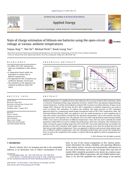
State of charge estimation of lithium-ion batteries using the open-circuit voltage at various ambienttemperaturesYinjiao Xing a ,⇑,Wei He b ,Michael Pecht b ,Kwok Leung Tsui aa Department of Systems Engineering and Engineering Management,City University of Hong Kong,83Tat Chee Avenue,Kowloon,Hong Kong bCenter for Advanced Life Cycle Engineering (CALCE),University of Maryland,College Park,MD 20740,USAh i g h l i g h t sg r a p h i c a l a b s t r a c t100020003000400050006000020406080Time(s)S O C (%)True & Estimated SOC [ambient temperature:40oC]True SOC Initial GuessEstimated SOC based on OCV-SOCEstimated SOC based on OCV-SOC-40°Ca r t i c l e i n f o Article history:Received 2April 2013Received in revised form 28June 2013Accepted 3July 2013Available online 7August 2013Keywords:Electric vehiclesLithium-ion batteries SOC estimationOpen-circuit voltageTemperature-based model Unscented Kalman filteringa b s t r a c tAmbient temperature is a significant factor that influences the accuracy of battery SOC estimation,which is critical for remaining driving range prediction of electric vehicles (EVs)and optimal charge/discharge control of batteries.A widely used method to estimate SOC is based on an online inference of open-circuit voltage (OCV).However,the fact that the OCV–SOC is dependent on ambient temperature can result in errors in battery SOC estimation.To address this problem,this paper presents an SOC estimation approach based on a temperature-based model incorporated with an OCV–SOC–temperature table.The unscented Kalman filtering (UKF)was applied to tune the model parameters at each sampling step to cope with various uncertainties arising from the operation environment,cell-to-cell variation,and mod-eling inaccuracy.Two dynamic tests,the dynamic stress test (DST)and the federal urban driving schedule (FUDS),were used to test batteries at different temperatures.Then,DST was used to identify the model parameters while FUDS was used to validate the performance of the SOC estimation.The estimation was made covering the major working range from 25%to 85%SOC.The results indicated that our method can provide accurate SOC estimation with smaller root mean squared errors than the method that does not take into account ambient temperature.Thus,our approach is effective and accurate when battery oper-ates at different ambient temperatures.Since the developed method takes into account the temperature factor as well as the complexity of the model,it could be effectively applied in battery management sys-tems for EVs.Ó2013Elsevier Ltd.All rights reserved.1.IntroductionElectric vehicles (EVs)are bringing new life to the automobile industry as an alternative way to reduce consumption of fossil fuels.As one of the critical components in EVs,battery perfor-mance determines the safety,reliability,and operating efficiency of the vehicle system.Accurate and instantaneous information on the state of the battery,such as state of charge (SOC)and state of health (SOH),should be provided to the drivers by a battery man-agement system (BMS)toguarantee safe and reliable battery oper-ation.[1–4].The SOC quantifies the usable energy at the present0306-2619/$-see front matter Ó2013Elsevier Ltd.All rights reserved./10.1016/j.apenergy.2013.07.008⇑Corresponding author.Tel.:+852********;fax:+852********.E-mail addresses:yxing3@.hk (Y.Xing),weihe@ (W.He),pecht@ (M.Pecht),kltsui@.hk (K.L.Tsui).cycle,while the SOH denotes the remaining performance of the battery over its whole life cycle[5].Battery SOC is a direct and immediate look at the remaining charge of the battery,which re-flects residual range of an EV.This has gained more attention due to drivers’range anxiety i.e.running out of power on the road. Additionally,an accurate SOC is an indicator of how to improve a battery’s operational reliability,extend its lifespan,and optimize the power management of the vehicle[1,2,6].However,SOC can-not be measured directly but must be estimated according to mea-surable parameters such as current and voltage.Moreover, ambient temperature is a critical factor that affects the accuracy of SOC estimation[7–12].There are three main types of methods for SOC estimation:cou-lomb counting,machine learning methods,and their combination using a model-based estimation approach.These three types of methods are described below.Coulomb counting is a straightforward method for estimating SOC that accumulates the net charge at the last time period in units of ampere-hours(Ah).Its performance is highly reliant on the pre-cision of current sensors and the accurate estimation of the initial SOC[3,13].However,coulomb counting is an open-loop estimator that does not eliminate the accumulation of measurement errors and uncertain disturbances.In addition,it is not able to determine the initial SOC,and address the variation of the initial SOC caused by self-discharging.Without the knowledge of the initial SOC,this method will cause accumulating errors on SOC estimation.Taking into account these factors,regular recalibration is recommended and widely used by methods such as fully discharging the battery, or referring to other measurements such as open-circuit voltage (OCV),as suggested in[3,6,7,14].Machine learning approaches,including artificial neural net-works,fuzzy logic–based models,and support vector machines, have been used to estimate SOC online.Li et al.[15]designed a 12-input-2-level merged fuzzy neural network(FNN)that was fused with a reduced-form generic algorithm(RGA)to estimate SOC.Bo et al.[16]developed parallel chaos immune evolutionary programming(PICEP)to train a neural network model in which five input variables were selected.This approach was used to esti-mate the SOC of nickel–metal hydride(Ni/MH)batteries.The per-formance of the kind of black-box models is reliant on the reliability of the training data,i.e.whether it is sufficient to cover the entire loading conditions.Once the battery operated at the un-known loading conditions,the robustness of these models was subject to challenge.Wang[17]employed a support vector ma-chine to model the dynamic behavior of a Ni/MH battery under dy-namic current loading.However,model training is time consuming and requires a large amount of data.Also,the estimation based on this model causes a large prediction error due to the uncertainty of the new data set.A model-basedfiltering estimation approach is being widely ap-plied due to its close-loop nature and concerning various uncer-tainties.Both electrochemical models and equivalent circuit models aim to capture the dynamic behavior of the battery.The former are usually presented in the form of partial differential equations with many unknown parameters.They are accurate but not desirable in practice because of a high requirement for memory and computation.To guarantee the accuracy of the model and the feasibility,equivalent circuit models have been imple-mented in BMSs such as the enhanced self-correcting(ESC)model and the hysteresis model,as found in[10,18,19],and one or two-order resistance–capacitance(RC)network models[1,2,10,11,20]. OCV is a vital element in the above-mentioned battery equivalent models and is a function of SOC in nature.The premise of utilizing OCV–SOC is that the battery needs to rest a long time and terminal voltage approaches the OCV.However,in real life,a long resting time may not be possible.To make up for theflaws of OCV meth-ods,nonlinearfiltering techniques based on state-space models have been developed to enhance SOC estimation through combin-ing coulomb counting and OCV[7].Plett applied extended Kalman filters(EKF)into BMS to implement SOC estimation of a lithium polymer battery(LiPB)using different battery models in [10,21,22].Plett later proposed the use of two sigma-point Kalman filtering(SPKF)estimators,including the unscented Kalmanfilter (UKF)and central difference Kalmanfilter(CDKF),in[18,23].Sub-sequently,adaptive EKF[7,20],dual EKF[11],and adaptive UKF[3] were developed to improve the accuracy of the SOC estimation based on their own sample sets and some common equivalent cir-cuit models.Charkhgard and Farrokhi[13]also proposed the com-bination of NN and EKF to estimate SOC.NN was employed to train a lithium-ion battery model using some charging data from the battery.The effectiveness of this method was not verified under the dynamic discharging data,which would lead to a larger uncer-tainty on estimating SOC.However,several existing issues are seldom addressed in the literature.Firstly,the temperature dependence of the OCV–SOC lookup table is seldom discussed with regard to battery SOC esti-mation.Instead,a single OCV–SOC table constructed at a certain temperature(e.g.,room temperature)is widely employed.It will cause a large error in inferring SOC when the battery is operating at other ambient temperatures(not room temperature) [1,8,10,11].Secondly,lithium-ion batteries have a relativelyflat OCV curve over the SOC,especially for lithium iron phosphate (LiFePO4)batteries,which are widely used in the electric vehicle market[24].That means a small error on the inferred OCV will produce a larger deviation in SOC.Thirdly,different models were adopted by individuals based on their own experimental data. Although a sophisticated model with more parameters might be able to provide a smaller modeling error,it would run the risk of adding more uncertainties,such as over-fitting problems and the introduction of unnecessary noises,especially concerning temperature.Therefore,it makes more sense to investigate a gen-eric but accurate temperature-based model with fewer parame-ters for real-time applications.Kim et al.[25]considered temperature as an input variable into afirst-order RC circuit model.However,the effect of temperature on the OCV–SOC was ignored due to a slight difference between OCV curves from 30%SOC to80%at different temperatures.Moreover,their samples have an obvious linear slope of OCV–SOC that is prone to infer SOC accurately.Nevertheless,for a relativelyflat OCV curve dependent on ambient temperature,it is significant not only to develop an accurate and generic model considering ambient temperature,but also to enhance the capability of online estimation due to the uncertainty,including unit-to-unit varia-tion,measurement noise,operational uncertainties,and model inaccuracy[26].In this paper,a temperature-based internal resistance(R int)bat-tery model combined with a nonlinearfiltering method was put forward to improve the SOC estimation of lithium-ion batteries un-der dynamic loading conditions at different ambient temperatures. The research proceeds as follows.Three tests at different tempera-tures are introduced in Section2.The dynamic stress test(DST)and federal urban driving schedule(FUDS)are two kinds of dynamic loading conditions tested at different temperatures to identify the model parameters and verify the estimated performance, respectively.The purpose of the OCV–SOC–temperature(OCV–SOC–T)test is to extend the OCV–SOC behavior to temperature field.Due to various uncertainties of the system,UKF-based SOC estimator is proposed due to its superiority of reaching to the 3rd order of any nonlinearity over the EKF.The implemented procedure for our battery study is followed by Section3.The experimental results are presented in Section4to compare our developed method based on OCV–SOC–T with the originalY.Xing et al./Applied Energy113(2014)106–115107estimation using a single OCV–SOC table.The robustness is vali-dated and compared under the different initial true values and dif-ferent initial guesses of SOC.2.ExperimentsThe experiment setup is shown in Fig.1.It consisted of (1)lith-ium-ion cells (LiFePO4)of the 18650cylindrical type (the key spec-ifications are shown in Table 1);(2)Vötsch temperature test chamber (The cells were placed in cell holders in the chamber);(3)a current and voltage sampling cable for loading and sampling;(4)a battery test system (Arbin BT2000tester);(5)a PC with Ar-bins’Mits Pro Software (v4.27)for battery charging/discharging control;(6)Matlab R2009b for data analysis.During battery oper-ation,the sampling time of current,voltage was 1s.Three separate test schedules were conducted on the battery test bench for model identification,OCV–SOC–T table construction,and method valida-tion,respectively.2.1.Model identification testFor model identification,the dynamic stress test (DST)was run from 0°C to 50°C at an interval of 10°C.DST is employed to investigate the dynamic electric behavior of the battery.It is designed by US Advanced Battery Consortium (USABC)to simu-late a variable-power discharge regime that represents the expected demands of an EV battery [27].A completed DST cycle is 360s long and can be scaled down to any desired maximum demand regarding the specifications of the test samples.There-fore,in our study,DST was run continuously from 100%SOC at 3.6V to empty at 2V over several cycles in a discharge process.The positive current responds to discharging while the negative denotes charging.The measured current and voltage profile at 20°C is shown in Fig.2.2.2.The OCV–SOC–T testOCV is a function of SOC for the cells.If the cell is able to rest for a long period until the terminal voltage approached the true OCV,OCV can be used to infer SOC accurately.However,this method is not practical for dynamic SOC estimation.To address this issue,the SOC can be estimated by combining the online identification of the OCV with the predetermined offline OCV–SOC lookup table.Taking into account the temperature dependence of the OCV–SOC table,the OCV–SOC test was conducted from 0°C to 50°C at an interval of 10°C.The test procedure at each temperature is the same as fol-lows.Firstly,the cell was fully charged using a constant current of 1C-rate (1C-rate means that a full discharge of the battery takes approximately 1h)until the voltage reached to the cut-off voltage of 3.6V and the current was 0.01C.Secondly,the cell was fully dis-charged at a constant rate of C/20until the voltage reached 2.0V,which corresponds to 0%SOC.Finally,the cell was fully charged at a constant rate of C/20to 3.6V,which corresponds to 100%SOC.The terminal voltage of the cell is considered as a close approximation to the real equilibrium potential [6,10].AsshownFig.1.Schematic of the battery test bench.Table 1The key specifications of the test samples.Type Nominal voltage Nominal capacity Upper/lower cut-off voltage Maximum continuous discharge current LiFePO 43.3V1.1Ah3.6V/2.0V30A010002000300040005000-2024Time (s)C u r r e n t (A )in Fig.3,the equilibrium potential during the charging process is higher than that during discharging process.It accounts for a hys-teresis phenomenon of the OCV during the charging/discharging.In our paper,the OCV curve was defined as the average value of the charge and discharge equilibrium potentials.The effect of the hys-teresis was ignored.In addition,referring to[28],when SOC is normalized relative to the specific cell capacity,the OCV–SOC curve can be referred to as being unique for the same type at the same testing condition.Fig.3shows the average OCV at20°C.A flat OCV slope between25%and80%SOC is emphasized in another small plot in Fig.3.Its effect will be discussed in Section3.1.2.3.Method validation testA validation test with a more sophisticated dynamic current profile,the federal urban driving schedule(FUDS),was conducted to verify the estimation algorithm based on the developed model. FUDS is a dynamic electric vehicle performance test based on a time–velocity profile from an automobile industry standard vehi-cle[27].In the laboratory test,a dynamic current sequence was transferred from the time–velocity profile,programmed to charge or discharge the battery and applied to battery performance test [3,17,20,29].Similar to the DST test,the current sequence is scaled tofit the specification of the test battery and the limitation of the testing system of Fig.1.The current profile of FUDS causes varia-tion of the SOC from fully charged at3.6V to empty at2V.The FUDS test was also run form0°C to50°C at an interval of10°C. The measured current,voltage profile,and the cumulative SOC at 20°C are shown in Fig.4.A completed FUDS current profile over 1372s is emphasized in another graph in Fig.4(a).3.Battery modelingFor lithium-ion batteries,the internal resistance(R int)model is generic and straightforward to characterize a battery’s dynamics with one estimated parameter.Although a sophisticated model with more parameters would possibly show a well-fitting result, such as an equivalent circuit model with several amounts of paral-lel resistance–capacitance(RC)networks,it would also pose a risk of over-fitting and introducing more uncertainties for online esti-mation at the same time.Especially taking into account tempera-ture factor,more complexity should be imposed on battery modeling.Therefore,we would prefer a simple model to a sophis-ticated model if the former had generalization ability and provided sufficiently good results.In this paper,model modification based on the original R int model is proposed to balance the model com-plexity and the accuracy of battery SOC estimation.The schematic of the original R int model is shown in Fig.5.U term;k¼U OCVÀI kÂRð1ÞU OCV/fðSOC kÞð2ÞIn Eqs.(1)and(2),U term,k is the measured terminal voltage of the battery under a normal dynamic current load at time k,and I k is the dynamic current at the same time.The positive current re-sponds to discharging while the negative value means charging.R is the simplified total internal resistance of the battery.U OCV is a function of SOC of the battery that should be tested following the procedure as presented in Section2.2.The battery model Eq.(1) can be used to infer OCV directly according to the measured termi-Schematic of the internal resistance(R int)modelY.Xing et al./Applied Energy113(2014)106–1151093.1.Model parameter identificationThe DST was run on the LiFePO4batteries to identify the model parameter R in Eq.(1).Taking the current and voltage profile of DST at20°C as an example,the voltage and current are measured and recorded from fully charged to empty with a sampling period of1s based on our battery test bench.The accumulative charge(exper-imental SOC)is calculated synchronously from100%SOC.Thus, the parameter R can befitted using a sequence of the current,volt-age,and the offline OCV–SOC by the least square algorithm.In terms of thefitted R value,the model performance can be evalu-ated based on the measured terminal voltage(U term,k)and the esti-mated voltage(U term;k).Fig.6shows the measured and the estimated voltage response on the DST profile at20°C based on the original model.In statistics,the mean absolute error(MAE)and the root mean squared(RMS)error can be used together to evaluate the good-ness-of-fit of the model.These two indicators are given by the fol-lowing equations respectively.MAE¼1X nk¼1j e k jð3ÞRMS error¼ffiffiffiffiffiffiffiffiffiffiffiffiffiffiffiffiffiffiffiffiffiffiffiffiffiffiffi1nX nk¼1ðe kÞ2rð4ÞHere,e k is the modeling error(U term,kÀU term;k)at time k.The MAE measures how close forecasts are to the corresponding out-comes without considering the direction.The RMS error is more sensitive to large errors than the MAE.It is able to characterize the variation in errors.The statistics list of the model is shown in Table2.According to the small graph in Fig.3,the OCV slope,namely, dOCV/dSOC is approximately equal to0.0014between25%and 80%SOC.This means that the deviation on the OCV inference will cause an estimated deviation of SOC up to21%when there is a MAE of0.0288V based on the current model.Additionally,a large mean error was plotted over time in Fig.6.Thus,the residuals should be reduced to improve the model adequacy with smaller MAE and RMS error values.3.2.Model improvement and validation3.2.1.The OCV–SOC–T table for model improvementAccording to the test in Section2.2,six OCV curves were ob-tained from0°C to50°C at an interval of10°C.Fig.7(a)empha-sizes the differences of OCV–SOC curves between30%and80% SOC at different temperatures.It can be seen that SOC0°C is much larger than other SOC values at higher temperatures when the OCV inference is the same,i.e.,3.3V.It makes sense that the releas-able capability of the charge is reduced at low temperatures. Fig.7(b)shows the SOC values if the OCV inference was equal to the specific values from3.28V to3.32V at intervals of0.01V at three temperatures:0°C,20°C,40°C.One issue of interest can be seen in Fig.7(b).That is,the same OCV inference at different temperatures corresponds to different SOC values.For example,the SOC difference between0°C and 40°C reaches approximately22%at an OCV of3.30V.Therefore, we propose adding the OCV–SOC–T to the battery model to im-prove the model accuracy.The improved battery model is as follows:U term;k¼U OCVðSOC k;TÞÀI kÂRðTÞþCðTÞð5Þwhere U OCV is a function of SOC and ambient temperature(T).C(T)is a function of temperature that facilitates the reduction of the offset due to model inaccuracy and environmental conditions.Fig.8 shows the measured and the estimated voltage response on the DST profile at20°C based on the proposed model.It can be found that the mean error of the new model is reduced with small varia-tions as compared to the original model in Fig.6.Another issue of interest in Fig.7(b)is that a small deviation of 0.01V in OCV inference will lead to a large difference in SOC at the same temperature condition.It is the same issue as shown in Fig.3. Therefore,if the SOC estimation were directly inferred from a bat-tery model,it would have a high requirement on the model and measurement accuracy.To address this issue and improve the accuracy of the SOC estimation,the model-based unscented Kal-manfiltering approach was employed and introduced in Section4.3.2.2.The validation of the proposed modelBased on the developed model in Eq.(5),it is noted that the spe-cific OCV–SOC look-up table should be selected in terms of the ambient temperature(here it is viewed as an average value).Least squarefitting was also used to identify model parameters,R and C. Thefitted model parameter list and the statistics list of the pro-posed model are shown in Table3.In comparison to thefitted results at20°C of Table2,here the MAE is one order of magnitude smaller than that of the original model and the RMS modeling error is also reduced.In addition, the correlation coefficient(Corrcoef)was calculated for residual analysis.The Corrcoef(e k,I k)values close to zero indicate that the residuals and the input variable hardly have linear relationship. Thus,the corrected model can be betterfitted on the dynamic cur-rent load.Onefinding of interest is C values that can befitted over the ambient temperature(T)using a regression curve,as Fig.9 shows.Referring to the paper[30],the exponential function can be selected tofit C values over T because the internal elements of the battery,i.e.,battery resistance follow the Arrhenius equation, which has exponential dependency on the temperature.In our study,five C values at0°C,10°C,20°C,25°C,30°C,40°C wereTable2Model parameter and statistics list of thefitted error of the model.R(X)Mean absolute error RMS modeling error0.24450.0288V0.0301110Y.Xing et al./Applied Energy113(2014)106–115used for curvefitting while C(50°C)was used to test thefitted per-formance of this exponential function.The95%prediction bounds are shown in Fig.9based on C values andfitted curve.Apparently, C(50°C)drops within the95%prediction bounds.It can be seen that the function of C(T)in Fig.9can be used to estimate C when the corresponding temperature test has not been run.4.Algorithm implementation for online estimationThe online SOC estimation has strong nonlinearity.This point can be seen from any battery model in which OCV has a nonlinear relationship with SOC.Additionally,the uncertainties due to the model inaccuracy,measurement noise,and operating conditions will cause a large variation in the estimation.The model-based nonlinearfiltering approach has been developed to implement dy-namic SOC estimation.The objective is to estimate the hidden sys-tem state,estimate the model parameters for system identification, or both.Thus,an error-feedback-based unscented Kalmanfiltering approach is proposed by shifting the system noise to improve the accuracy of the estimation.4.1.Unscented KalmanfilteringThe extended Kalmanfiltering(EKF)technique has become a popular technique for addressing the issue of state or parameter estimation for nonlinear systems.The rationale behind EKF is still the KF approach based on state space modeling.It aims to utilize the error between the current measurement and the model output to adjust the model state by virtue of a Kalman gain.Its principle and implementation can be found in[31].Since KF is only available for linear systems,extended Kalmanfiltering(EKF)used a lineari-zation process at each time step to approximate a nonlinear system through thefirst-order Taylor series expansion[31,32].However, thefirst order approximation will probably lead to large errors inTable3Fitted model parameter list and statistics list of modelfitting.T(°C)R(X)C Mean absoluteerrors(V)RMSmodelingerrorsCorrcoef(e k,I k)00.2780À0.05520.01530.0188 1.36eÀ13100.2396À0.04360.01120.01348.45eÀ14200.2249À0.03600.00870.0105 1.09eÀ13250.2020À0.03260.00800.0095 1.02eÀ13300.1838À0.02890.00730.0085À7.62eÀ13400.1565À0.02370.00600.0071 2.85eÀ13500.1816À0.02010.00990.0131 3.15eÀ14Y.Xing et al./Applied Energy113(2014)106–115111the true posterior mean and covariance of the noise and could even result in divergence of thefilter.Under this situation,unscented Kalmanfiltering(UKF)based on unscented transformation was suggested to avoid the weakness that comes from using Taylor ser-ies expansion.The core idea of UKF is easier to approximate the state distribu-tion that is represented by a minimal set of chosen sample points called sigma points,which can capture the mean and covariance of Gaussian random variable when propagated through a nonlinear system.The state-space model of a nonlinear system is represented as follows:x k¼fðx kÀ1;u kÀ1Þþw kÀ1yk¼hðx k;u kÞþm kð6Þwhere x k is the system state vector and y k is the measurement vec-tor at time k.Correspondingly,f(Á)and h(Á)are the state function and the measurement function,respectively;u k is the known input vector;w k$Nð0;PwÞis the Gaussian process noise;and v k$Nð0;PVÞis the Gaussian measurement noise.Assume the state x has mean x and covariance P ing the unscented transformation (UT),the state will be transformed as a matrix of2n+1sigma vec-tors v i with corresponding weights w i.These sigma points are shown in the following equation:vkÀ1¼½ xð0ÞkÀ1; xð1:nÞkÀ1; xðnþ1:2nÞkÀ1¼½ x kÀ1; x kÀ1þffiffiffiffiffiffiffiffiffiffiffiffiffiffiffiffiffiffiffiffiffiffiffiffiffiðnþkÞP kÀ1p; x kÀ1ÀffiffiffiffiffiffiffiffiffiffiffiffiffiffiffiffiffiffiffiffiffiffiffiffiffiðnþkÞP kÀ1pð7Þwhere n is the dimension of the state and k is a scaling parameter. These sigma points are propagated through a nonlinear function,re-estimated,and then they are used to capture the posterior mean and covariance to the3rd Taylor expansion,as shown in Eqs.(9) and(10).yi¼hðv iÞ;i¼0;...;2nð8Þ y%X2ni¼0wðiÞmyið9ÞP y%X2ni¼0wðiÞcf y iÀ y gf y iÀ yg Tð10Þwhere wðiÞm and wðiÞc are the weights of the corresponding sigma points that can be calculated in[33–35]for details.4.2.SOC estimation based on proposed methodIn our battery study,the state vector is x=[SOC,R]T.Thefirst state equation in Eq.(11)follows the coulomb counting method mentioned in Section1.Peukert effect and capacity aging could be partially compensated when introducing the process noise x1,kÀ1.A random walk is applied to the model parameter R regard-ing the cell-to-cell variation and operation uncertainties.Tuning the R will also be able to compensate for the variation of the C in our proposed model.The terminal voltage of the battery is the measured vector y=U term,that is,the proposed battery model as shown in Eq.(5).State function:SOC k¼SOC kÀ1ÀI kÀ1ÂD t=C nþx1;kÀ1R k¼R kÀ1þx2;kÀ1ð11ÞMeasurement function:U term;k¼U OCVðSOC k;TÞÀI kÂR kðTÞþCðTÞþm kð12Þwhere I k is the current as the input(u k in Eq.(6))at time k;D t is the sampling interval,which is1s according to the sampling rate;and C n is the rated capacity.The rated capacity of the test samples is1.1 Ah.And x1,k,x2,k and m k are zero-mean white stochastic processes with covariancesPx1,Px2andPm,respectively.According to the proposed state-space model in Eqs.(11)and(12),the procedure of SOC estimation based on UKF is summarized in Table4.Table4Summary of the UKF approach for SOC estimation.Initialize:–Measure ambient temperature,prepare U OCV(SOC,T)and R0,C0–Initial guess:S0,–Covariance matrix:P o–Process and measurement noise covariance:Pw0;PVGenerate sigma points at time kÀ1,(k2½l;...;1 ):vkÀ1¼S kÀ1R kÀ1¼½ v kÀ1; v kÀ1þffiffiffiffiffiffiffiffiffiffiffiffiffiffiffiffiffiffiffiffiffiffiffiffiffiðnþkÞP kÀ1p; v kÀ1ÀffiffiffiffiffiffiffiffiffiffiffiffiffiffiffiffiffiffiffiffiffiffiffiffiffiðnþkÞP kÀ1pPredict the prior state mean and covariance–Calculate sigma points through state function:v ik j kÀ1¼S i k j kÀ1R ik j kÀ1"#¼S i kÀ1ÀI kÀ1ÂD tC nR i kÀ1"#;i¼1; (2)–Calculate the prior mean and covariance:^xÀk ¼P2ni¼0w imv ik j kÀ1;PÀk¼P2ni¼0w ichv ik j kÀ1À^xÀkihv ik j kÀ1À^xÀki TþPwUpdate using the measurement function–Calculate sigma points y k j kÀ1¼U OCVðS k j kÀ1;TÞÀI kÂRðTÞk j kÀ1þCðTÞ–Calculate the propagated mean:^yÀk ¼P2ni¼0w i m y ik j kÀ1–Calculate the covariance of the measurement:P yÀk ;yÀk¼P2ni¼0w j c½y ik j kÀ1À^yÀkTþPm–Calculate the cross-covariance and the state and measurement:of battery SOC estimation by UKF112Y.Xing et al./Applied Energy113(2014)106–115。

第47卷第2期2021年4月航空发动机AeroengineVol.47No.2Apr.2021自适应变循环发动机性能优势评价方法李瑞军，王靖凯，吴濛（中国航发沈阳发动机研究所，沈阳110015）摘要：为了综合评价自适应变循环发动机相比常规涡扇发动机的性能优势，提出了从发动机耗油率降低和质量增加2个维度以及从发动机耗油率、飞机燃油消耗量和燃油效率之间关系的角度来评价自适应变循环发动机性能的2种方法。

结果表明：发动机耗油率降低和质量增加之间存在某个平衡点，只有质量增加幅度小于耗油率降低幅度时，才能体现自适应变循环发动机的性能优势，并且飞机航程越长，越能体现自适应变循环发动机耗油率降低带来的优势；发动机耗油率、飞机燃油消耗量和燃油效率之间呈指数关系变化，当假设飞机巡航航程为3500km 、飞机升阻比为10.5时，自适应变循环发动机巡航耗油率相比常规涡扇发动机的降低1%，可使飞机燃油消耗量减少约1.9%，飞机燃油效率提高约2.4%。

关键词：自适应变循环发动机；燃油消耗量；燃油效率；耗油率；性能优势；评价方法中图分类号：V231文献标识码：Adoi ：10.13477/ki.aeroengine.2021.02.003Performance Advantage Evaluation Method of Adaptive Variable Cycle EngineLI Rui-jun ，WANG Jing-kai ，WU-Meng（AECC Shenyang Engine Research Institute ，Shenyang 110015，China ）Abstract ：In order to comprehensively evaluate the performance advantages of adaptive variable cycle engines compared with conventional turbofan engines ，two methods for evaluating the performance of adaptive variable cycle engines were proposed from two dimensions of engine specific fuel consumption reduction and mass increase and the perspective of the relationship between engine specific fuel consumption ，aircraft fuel consumption and fuel efficiency.The results show that there is a balance point between thedecrease of engine specific fuel consumption and the increase of engine mass.Only when the increase of mass is less than the decrease ofspecific fuel consumption can the performance advantages of adaptive variable cycle engine be reflected.The longer the flight ，the better the advantages of the reduced specific fuel consumption of the adaptive variable cycle engine.The relationship between engine specific fuel consumption and aircraft fuel consumption and fuel efficiency is exponential.Assuming that the aircraft cruise range is 3500km and the lift-to-drag ratio is 10.5，the cruise specific fuel consumption of adaptive variable cycle engine can be reduced by 1%compared with that of the conventional turbofan engine ，which can reduce the aircraft fuel consumption by about 1.9%and increase the aircraft fuel efficiency by about 2.4%.Key words ：adaptive variable cycle engine ；fuel consumption ；fuel efficiency ；specific fuel consumption ；performance advantages ；evaluation method收稿日期：2020-03-06基金项目：航空动力基础研究项目资助作者简介：李瑞军（1979），男，硕士，自然科学研究员，主要从事航空发动机总体性能设计工作；E-mail ：***************。

基于天然气自热重整的SOFC系统性能分析李裕;叶爽;王蔚国【摘要】The target of this study is to investigate the performance and efficiency of an integrated autothermal reforming and SOFC (solid oxide fuel cell) system fueled by methane. A zero dimensional SOFC stack model, which consists of electrochemical reactions and thermodynamics, is developed by Fortran and validated with experiment results, and links it to Aspen Plus software as a subroutine. Based on mass and energy balances, influences of steam to carbon(S/C) ratio and fuel utilization(Uf) on performance of SOFC power systems are investigated. The simulation results show that increase in the S/C ratio can enhance hydrogen production while reduce CO formation. Oxygen to carbon ratio and system efficiency achieve maximum when S/C ratio is 1.5. Increase of fuel utilization can enhance current density, resulting in increase of excess air ratio and decrease of air utilization. The overall efficiency and electric efficiency of the system all are increase because more chemical energy is converted into electric energy, whose maximum values are 44.5% and39.2%, respectively. The performance characteristics obtained is of great significance for further optimization of integrated SOFCsystems&nbsp;with autothermal reforming of natural gas.%建立一个天然气自热重整的固体氧化物燃料电池（SOFC）系统模型，利用Aspen Plus化工流程模拟软件链接基于Fortran语言编写的电堆模型，在质量守恒和能量守恒的基础上，分析不同参数对系统性能的影响。

第３６卷㊀第４期２０１８年１０月㊀㊀㊀㊀广西师范大学学报(自然科学版)J o u r n a l o fG u a n g x iN o r m a lU n i v e r s i t y (N a t u r a l S c i e n c eE d i t i o n )㊀㊀㊀㊀㊀㊀V o l ．３６㊀N o ．４O c t ．２０１８D O I :１０．１６０８８/j ．i s s n ．１００１Ｇ６６００．２０１８．０４．００４h t t p ://x u e b a o ．gx n u ．e d u ．c n 收稿日期:２０１７Ｇ０９Ｇ１０基金项目:国家自然科学基金(６１３６１０１１)通信联系人:宋树祥(１９７０ ),男,湖南双峰人,广西师范大学教授,博士.E Ｇm a i l :s o n g s h u x i a n g ＠m a i l b o x ．gx n u ．e d u ．c n 基于随机森林的锂离子电池荷电状态估算韦振汉,宋树祥∗,夏海英(广西师范大学电子工程学院,广西桂林５４１００４)摘㊀要:荷电状态(s t a t e Ｇo f Ｇc h a r g e ,S O C )是锂离子电池预测和健康管理非常重要的一部分.锂离子电池的S O C 无法直接测量,因此本文提出了基于随机森林回归算法的锂离子电池S O C 估计的方法.首先构建随机森林回归模型,使用电池电流㊁电池电压㊁电池温度作为模型的训练输入,相对应的S O C 作为模型的训练输出;然后使用随机森林算法进行模型训练;最后将训练模型应用于电池S O C 估计.实验结果表明,随机森林回归算法对锂离子电池荷电状态的预测最大估算误差为０．０２,均方根误差为０．００３２０４,该方法能有效地估算锂离子电池S O C 并且有很高的估计精度.该模型研究为未来电池荷电状态估算系统的模型构建提供了参考.关键词:锂离子电池;随机森林回归;荷电状态(S O C )估计中图分类号:T P ３０１．６㊀㊀㊀文献标志码:A㊀㊀㊀文章编号:１００１Ｇ６６００(２０１８)０４Ｇ００２７Ｇ０７引用格式:韦振汉,宋树祥,夏海英．基于随机森林的锂离子电池荷电状态估算[J ]．广西师范大学学报(自然科学版),２０１８,３６(４):２７Ｇ３３．W E I Z h e n h a n ,S O N G S h u x i a n g ,X I A H a i y i n g ．S t a t e Ｇo f Ｇc h a r g ee s t i m a t i o nu s i n g r a n d o mf o r e s t f o r l i t h i u mi o nb a t t e r y [J ]．J o u r n a l o fG u a n g x iN o r m a lU n i v e r s i t y(N a t u r a l S c i e n c eE d i t i o n ),２０１８,３６(４):２７Ｇ３３．S t a t e Ｇo f Ｇc h a r g eE s t i m a t i o nU s i n g R a n d o m F o r e s t f o rL i t h i u mI o nB a t t e r yW E IZ h e n h a n ,S O N GS h u x i a n g ∗,X I A H a i y i n g(C o l l e g e o fE l e c t r o n i cE n g i n e e r i n g ,G u a n g x iN o r m a lU n i v e r s i t y ,G u i l i nG u a n g x i ５４１００４,C h i n a )A b s t r a c t :S t a t e Ｇo f Ｇc h a r g e (S O C )i sav e r y i m p o r t a n t p a r to f l i t h i u m Ｇi o nb a t t e r yp r e d i c t i o na n dh e a l t h m a n a g e m e n t ．A st h eS O Co f t h el i t h i u m b a t t e r y c a n n o tb e m e a s u r e dd i r e c t l y ,t h i s p a p e r p r e s e n t sa m e t h o do fe s t i m a t i n g t h eS O Co f t h e l i t h i u m Ｇi o nb a t t e r y b y t h er a n d o mf o r e s t r e g r e s s i o n ．F i r s t l y ,a r a n d o m f o r e s tr e g r e s s i o n m o d e li s c o n s t r u c t e d ．T h e b a t t e r y c u r r e n t ,b a t t e r y v o l t a g e a n d b a t t e r y t e m p e r a t u r e a r eu s e da st h et r a i n i n g i n p u to f t h e m o d e l ,a n dt h ec o r r e s p o n d i n g S O Ci su s e da st h e t r a i n i n g o u t p u t o f t h em o d e l ．A n dt h e n ,t h e r a n d o mf o r e s t a l g o r i t h mf o rm o d e l t r a i n i n g i sc o n d u c t e d ．F i n a l l y ,t h et r a i n i n g m o d e l i sa p p l i e dt ot h eb a t t e r y S O Ce s t i m a t i o n ．T h er e s u l t ss h o wt h a tb y t h e r a n d o mf o r e s t r e g r e s s i o na l g o r i t h m ,t h em a x i m u me s t i m a t i o ne r r o r o f t h e l i t h i u m Ｇi o nb a t t e r y c h a r g e i s ０．０２,a n d t h eR M S Ei s ０．００３２０４．T h i sm e t h o dc a ne f f e c t i v e l y e s t i m a t e t h e l i t h i u m Ｇi o nb a t t e r y S O Ca n d h a s h i g he s t i m a t i o na c c u r a c y ．T h i sm o d e lm a yp r o v i d ea r e f e r e n c e f o r t h em o d e l c o n s t r u c t i o no f f u t u r e b a t t e r y c h a r g e e s t i m a t i o n s y s t e m．K e yw o r d s :l i t h i u m Ｇi o nb a t t e r y ;r a n d o mf o r e s t r e g r e s s i o n ;s t a t e Ｇo f Ｇc h a r g e (S O C )e s t i m a t i o n 相对于可充电镍镉电池与镍氢电池,锂离子电池具有密度高㊁使用寿命长㊁工作电压高㊁无环境污染等８２广西师范大学学报(自然科学版),２０１８,３６(４)优点.因此,锂离子电池被广泛应用于各种便携式信息处理终端㊁电动汽车等领域.随着锂离子电池的广泛应用,电池荷电状态(s t a t eＧo fＧc h a r g e,S O C)估计已成为一个越来越重要的问题,这是因为准确的S O C 估计在用户充电之前显示电池的可用性,防止电池出现过充电或充电不足等问题,从而延长电池的寿命[１].然而,S O C不能直接测量,必须通过测量电压㊁电流与温度等参数进行估计得到[２].目前有几种算法用来估算锂离子电池的S O C,包括安倍时计数法㊁开路电压法㊁人工神经网络算法[３Ｇ５].安倍时计数法简单易用,但存在初始误差和累积误差的问题[３].开路电压法准确估计锂离子电池S O C,但只能在电池停止工作后很长一段时间进行测量,因此此算法不适合在线估计[４].人工神经网络是一种基于电池历史数据的黑盒方法,利用其非线性特性训练大量的数据来估算锂离子电池的S O C.锂离子电池S O C的估算有很多影响因素,如电池电压㊁电流㊁温度㊁电池内部电化学反应等,如果有太多的因素选择,将导致计算量庞大,同时不能正确反映锂离子电池的S O C[５].此外,人工神经网络算法对维度差异的影响因素非常敏感,要求输入变量规范化,也存在过学习㊁容易陷入局部最小值等问题[６].目前,主成分分析(p r i n c i p a l c o m p o n e n t a n a l y s i s,P C A)通过分析影响电池的重要性因素来选择合适的影响因素模型,但这一过程需要大量的时间[７].为了解决安倍时计数法㊁开路电压法以及人工神经网络算法等存在的问题[８],本文提出基于随机森林回归的方法来估计S O C.随机森林回归算法不但具有分析特征重要性的能力,而且还能有效地避免过拟合现象,在没有增加计算量的情况下解释数以百计的影响因素[９].１㊀随机森林概述１．１㊀决策树J．R．Q u i n l a n提出了I D３决策树算法[１０],L．B r e i m a n等提出了分类回归树(c l a s s i f i c a t i o na n d r e g r e s s i o n t r e e s,C A R T)算法[１１],１９９３年Q u i n l a n又提出了C４．５决策树算法[１２].这３种算法均采用自上而下的贪婪算法构建一个树状结构,在每个内部节点选取一个最优的属性进行分裂,每个分枝对应一个属性值,如此递归建树直到满足终止条件,每个叶节点表示沿此路径的样本的所属类别.决策树不需要先验知识,相比神经网络等方法更容易解释,但是由于决策树在递归的过程中,可能会过度分割样本空间,最终建立的决策树过于复杂,导致过拟合的问题,使得分类精度降低.为避免过拟合问题,需要对决策树进行剪枝,根据剪枝顺序不同,分为事先剪枝方法和事后剪枝方法,但这２种方法都会增加算法的复杂性.１．２㊀随机森林回归随机森林回归由L．B r e i m a n提出[１３Ｇ１４].随机森林回归由回归树{h(X,θk),k＝１, ,K}构成,其中K为随机森林所包含的决策树个数.原样本集T为{(x i,y i),x iɪX,y iɪY,i＝１,２, ,N},其中N为样本容量,X是观察的输入向量,Y是所对应的输出值,X和θk是独立的同分布随机向量.假设训练数据服从独立联合分布(X,Y),那么随机森林预测值H(x)表示为:H(x)＝(１/K)ðk k＝１h(x,θk),(１)定义随机森林均方泛化误差为:E X,Y(Y－h(x))２.(２)当Kңɕ,根据大数定律确保:E X,Y(Y－h(x))２ңE X,Y(Y－Eθh(X,θ)),(３)式(３)右边的式子是随机森林的泛化误差,表示为P E∗(f o r e s t).式(３)的收敛性表示随机森林并没有过拟合.假设对于所有的θ,有E(Y)＝E X h(X,θ),那么P E∗(f o r e s t)ɤρEθE(X,Y)(Y－h(X,θ)２,(４)式(４)中,EθE(X,Y)(Y－h(X,θ)２表示决策树平均泛化误差,表示为P E∗(t r e e);ρ表示残差Y－h(X,θ)与Y －h(X,θᶄ)加权之间的相关性,θ与θᶄ相互独立.从式(４)可以看出,为了确保随机森林预测的准确性,必须９２h t t p://x u e b a o．g x n u．e d u．c n降低森林成员之间的相关性和泛化误差.本文通过调整ρ来降低森林树木之间的相关性和泛化错误.２㊀基于随机森林的锂离子电池荷电状态估算建模建立基于随机森林回归的锂离子电池荷电状态估算模型的步骤如下:①设θ为随机参数向量,决定回归树的生长,对应的决策树记为T(θ),记决策树T(θ)的叶节点为L(x,θ).所示.图１㊀决策树的训练过程F i g．１㊀T r a i n i n gp r o c e s s o f d e c i s i o n t r e e②采取b o o t s t r a p方法重采样随机产生M个训练集,生成对应的决策树{T(x,θ１)},{T(x,θ２)}, , {T(x,θM)}.构建数量为M的森林,森林的构建算法如下:输入:训练集D＝{(x１,y１),(x２,y２), ,(x N,y N)}输出:随机森林{T(x,θ１)},{T(x,θ２)}, ,{T(x,θM)}F o r i＝１ʒM１)从训练集D采用B o o t s t r a p重采样选出N个样本.２)从所有属性中随机选择K个属性.３)选择最佳分割属性.４)建立C A R T决策树.e n d.③假设特征向量为K维,从中随机抽取k个特征作为当前节点的分裂特征集,并以这k个特征中最好的分裂方式对该节点进行分裂.④每个回归树不进行剪枝得到最大限度的生长.⑤对于一个新的数据X＝x,单颗决策树T(θ)的预测通过叶节点L(x,θ)的观测值取平均获得.令权重向量ωi(x,θ)为:ωi(x,θ)＝１{X iɪR l(x,θ)}＃{j:X j(x,θ)},(５)式(５)中,观测值x i属于叶节点L(x,θ)且不为零,权重ωi(x,θ)之和等于１.⑥在给定自变量X＝x下,单颗决策树的预测通过因变量的观测值σ(x):σ(x)＝ðn i＝１ωi(x,θ)Y i.(６)⑦通过对回归树权重ωi(x,θ)(t＝１,２, ,k)取平均,得到每个观测值iɪ(１,２, ,n)的权重广西师范大学学报(自然科学版),２０１８,３６(４)ωi (x ):ωi (x )＝k －１ðk i ＝１ωi (x ,θt )y .(７)⑧对所有的y ,随机森林的预测值μ(x ):μ(x )＝ðni ＝１ωi (x )Y i .(８)根据随机森林的算法步骤构造的模型如图所示.图２㊀基于随机森林的S O C 估算模型F i g ．２㊀S O Ce s t i m a t i o n b a s e o nR a n d o mf o r e s tm o d e l ３㊀实验结果与分析３．１㊀实验数据集本文采用随机森林回归算法对锂离子电池稳态放电过程S O C 进行估算.实验数据从一组锂离子电池的放电过程收集,数据下载于N A S A 艾姆斯研究中心[１５].用于实验的锂离子电池参数如表１所示.表１㊀锂离子电池参数T a b ．１㊀L i t h i u m Ｇi o nb a t t e r ypa r a m e t e r s ㊀㊀㊀参数数值额定容量/m A h 放电初始电压/V 放电截止电压/V 环境温度/ħ放电电流/A２０００４．２２．５２４２０３h t t p ://x u e b a o ．g x n u ．e d u ．cn 图３㊀放电数据F i g ．３㊀D i s c h a r g e d a t a 整个放电过程所记录的S O C 通过式(９)来计算:S O C ＝S O C ０＋１C R ʏt t ０I c m d τ,C R ＝ʏt E D V ０I c m d τ,(９)式(９)中,S O C ０是初始荷电状态,C R 是额定容量,I c m 是放电电流,t E D V 是当放电电压达到截止电压时的放电时间.３．２㊀实验结果与分析使用均方根误差(r o o t Ｇm e a n Ｇs q u a r e e r r o r ,R M S E )来评估随机森林回归估计的准确性.R M S E 定义如下:δR M S E ＝１n ðn i ＝１|f (x i )－y i |２,(１０)在式(１０)中,f (x i )是基于模型的估计值,yi 是S O C 真实值,n 是估计点的数量.在稳定的放电实验过程中,使用的数据为N A S A 艾斯卓越数据库预测中心提供的锂离子电池数据,４个锂离子电池组(＃５㊁＃６㊁＃７㊁＃１８)通过充电㊁放电和阻抗３种不同的操作得到.本文使用＃５组锂离子电池的放电数据来作为实验数据基础.在＃５数据集中,第１组到第４组放电数据作为模型的训练集,第７组放电数据用于模型的精度估算,第７组放电过程的数据(电压㊁电流㊁温度和S O C )如图３所示.电池电压㊁电流㊁温度被用作模型的特征输入,相应的S O C 值用作模型输出,这种变化主要是与之前的采样点比较.随机森林树的数量设置为５００(测试结果显示该模型能够保证收敛),随机选取的特征设置为２.为了验证随机森林回归算法在锂离子电池S O C 估计过程中的评估性能,B P 神经网络与T ＧS 模糊神经网络同时采用相同的参数作为基准进行对比.得到的第７组实验预测结果以及实验误差如图４所示.图４表明随机森林㊁B P 神经网络和T ＧS 模糊神经网络都具有较高的估计精度,与B P 神经网络和T ＧS 模糊神经网络相比,随机森林的S O C 预测几乎接近真实值.B P 神经网络和T ＧS 模糊神经网络估计误差随输入向量的变化误差处于较大的范围,随机森林可以确保误差在一定范围内.从图４(d)可以看出,随机森林㊁B P 神经网络和T ＧS 模糊神经网络的最大估算误差分别为０．０２㊁０．０２２与０．０２７.通过MA T L A B 平台仿真实验结果得出,随机森林㊁B P 神经网络和T ＧS 模糊神经网络的均方根误差(R M S E )分别为０．００３２０４㊁０．０４４５６９与０．０１８３２１.模型输入特征的重要性如图５所示.从图５可以看出,不论是对于精度或者基尼指数的影响,电压对锂离子电池荷电量估算的影响最大,温度对荷电量估算的影响其次,电流对荷电量的影响几乎为零,因此模型的特征重要性:电压＞温度＞电流.１３广西师范大学学报(自然科学版),２０１８,３６(４)图４㊀第７组实验预测结果F i g ．４㊀G r o u p ７e x p e r i m e n t a l p r o d i c t i o n r e s u l ts 图５㊀输入特征的重要性F i g ．５㊀T h e i m p o r t a n c e o f i n p u t f e a t u r e s 袋外错误率如图６所示.从图６可以看出,随着随机森林回归树的增加,袋外错误率逐渐处于一个平稳的状态,也就是说当回归树达到一定数量时,估算的误差结果将不会有太大的提高.在往后的研究中,可通过设置森林中树木的数量来减少迭代次数,进而减少模型运行时间.图６㊀袋外错误率F i g ．６㊀O u t Ｇo f Ｇb a g e r r o r r a t e ２３３３h t t p://x u e b a o．g x n u．e d u．c n４㊀结束语本文提出了利用随机森林回归算法进行锂离子电池S O C估计的方法.研究结果表明:与B P神经网络㊁TＧS神经网络算法相比,随机森林回归算法在估算电池荷电量时具有更高的精度;在估算样本数量有限的情况下,随机森林回归算法能有效地避免过拟合问题;随机森林算法的变量重要性分析可以分析特征的重要性程度这能在测量参数时通过提高参数的准确性,从而提高结果的估算精度;随机森林回归算法在处理具有噪声的数据时具有更好的鲁棒性.本文的随机森林回归算法可以用来估算锂离子电池的S O C,为未来锂离子电池荷电估算系统的模型构建提供了参考.参㊀考㊀文㊀献:[１]㊀姜琳．锂离子电池荷电状态估计与寿命预测技术研究[D]．成都:电子科技大学,２０１３．[２]㊀余升．电动汽车电池管理系统S O C估计算法研究[D]．合肥:合肥工业大学,２０１３．[３]㊀WA A G W,F L E I S C H E R C,S A U E R D U．C r i t i c a l r e v i e wo f t h em e t h o d s f o rm o n i t o r i n g o f l i t h i u mＧi o nb a t t e r i e s i ne l e c t r i c a n dh y b r i dv e h i c l e s[J]．J o u r n a l o fP o w e r S o u r c e s,２０１４,２５８:３２１Ｇ３３９．[４]㊀L E ES,K I MJ,L E EJ,e t a l．S t a t eＧo fＧc h a r g e a n dc a p a c i t y e s t i m a t i o no f l i t h i u mＧi o nb a t t e r y u s i n g an e wo p e nＧc i r c u i t v o l t a g e v e r s u s s t a t eＧo fＧc h a r g e[J]．J o u r n a l o fP o w e r S o u r c e s,２００８,１８５(２):１３６７Ｇ１３７３．[５]㊀Y A N Q i y a n,WA N G Y a n n i n g．P r e d i c t i n g f o r p o w e rb a t t e r y S O Cb a s e do nn e u r a l n e t w o r k[C]//２０１７３６t hC h i n e s eC o n t r o l C o n f e r e n c e．P i s c a t a w a y N J:I E E EP r e s s,２０１７:４１４０Ｇ４１４３．[６]㊀L I U F,L I U T,F U Y．A n I m p r o v e dS O Ce s t i m a t i o na l g o r i t h mb a s e do na r t i f i c i a l n e u r a l n e t w o r k[C]//I n t e r n a t i o n a l S y m p o s i u mo nC o m p u t a t i o n a l I n t e l l i g e n c e a n dD e s i g n．P i s c a t a w a y N J:I E E EP r e s s,２０１６:１５２Ｇ１５５．[７]㊀赵海霞,武建．浅析主成分分析方法[J]．科技信息,２００９(２):８７Ｇ８７．[８]㊀李亚林．动力电池荷电状态估算方法浅析[J]．汽车实用技术,２０１７(１８):１２０Ｇ１２１．[９]㊀石婷婷．基于随机森林算法的短期负荷预测研究[D]．郑州:郑州大学,２０１７．[１０]㊀Q U I N L A NJR．I n d u c t i o no f d e c i s i o n t r e e s[J]．M a c h i n eL e a r n i n g,１９８６,１(１):８１Ｇ１０６．[１１]㊀E V E R I T TBS．C l a s s i f i c a t i o na n d r e g r e s s i o n t r e e s[M]//E n c y c l o p e d i ao fS t a t i s t i c s i nB e h a v i o r a l S c i e n c e．H o b o k e n, N J:J o h n W i l e y&S o n s,L t d,２００５:１７Ｇ２３．[１２]㊀Q U I N L A NJR．C４．５:p r o g r a m s f o rm a c h i n e l e a r n i n g[M]．S a nF r a n c i s c o:M o r g a nK a u f m a n nP u b l i s h e r s I n c,１９９２．[１３]㊀B R E I MA NL．R a n d o mf o r e s t[J]．M a c h i n eL e a r n i n g,２００１,４５:５Ｇ３２．[１４]㊀S E G A L M R．M a c h i n e l e a r n i n g b e n c h m a r k sa n dr a n d o mf o r e s t r e g r e s s i o n[E B/O L]．(２００４Ｇ０４Ｇ１４)[２０１７Ｇ０９Ｇ１０]．h t t p://e s c h o l a r s h i p．o r g/u c/i t e m/３５x３v９t４．[１５]㊀S A HA B,G O E B E L K．N A S A A m e s p r o g n o s t i c sd a t ar e p o s i t o r y:b a t t e r y d a t as e t[D S/O L]．M o f f e t tF i e l d,C A: N A S A A m e s R e s e a r c h C e n t e r,２００７[２０１７Ｇ０９Ｇ１０]．h t t p s://t i．a r c．n a s a．g o v/t e c h/d a s h/p c o e/p r o g n o s t i cＧd a t aＧr e p o s i t o r y．(实习编辑㊀李㊀朝)。

NBU分布类的拟合优度检验(英文)
张道智
【期刊名称】《应用数学》
【年(卷),期】1989(2)3
【摘要】一个寿命分布F称为属于新的比旧的好的分布类(NBU),若:
R(x+y)≤R(x)R(y) x,y≥0这里R(x)=1-F(x)。

若R(x+y)≥R(x)R(y),称作旧的比新的好(NWU)。

本文讨论可靠性中应用非常广泛的NBU分布类的检验问题,即下列检验问题:原假设H_0:F是NBU的。

备选假设H_A:F不是NBU。

给出了检验函数。

并证明了备选假设是H_A:F是NWU时,检验是无偏的。

【总页数】6页(P59-64)
【关键词】NBU分布类;拟合优度;检验;寿命分布
【作者】张道智
【作者单位】机电部系统工程研究所
【正文语种】中文
【中图分类】O212.1
【相关文献】
1.寿命分布的参数 Bootstrap 拟合优度检验方法 [J], 孙权;周星;冯静;潘正强
2.基于拟合优度检验的客户贡献量分布研究 [J], 杨娅雯;马明;白静盼
3.一类上界型拟合优度检验统计量的精确分布 [J], 张军舰;李国英;赵志源
4.浅谈分布数据的x2拟合优度检验 [J], 张莹;李瑶瑶
5.多元正态分布的一个特殊积分和拟合优度检验 [J], 丁勇
因版权原因，仅展示原文概要，查看原文内容请购买。

基于深度学习的水力发电预测
陈颖光
【期刊名称】《电力系统装备》
【年(卷),期】2022()7
【摘要】精准的水力发电预测有助于安排检修计划等。

为此,文章提出一种基于门控循环单元的水力发电预测模型。

首先,采用自适应噪声的完全集合经验模态分解将原始水力发电序列分解为多个序列分量;接着,运用样本熵对所有分量进行复杂度分析后对序列分量进行重构;最后,对重构后的序列分量分别构建门控循环单元进行预测,将所有预测结果进行重构获得最终的预测结果。

结合实际算例分析,验证了本文所提模型的有效性。

【总页数】3页(P90-91)
【作者】陈颖光
【作者单位】福建华电金湖电力有限公司
【正文语种】中文
【中图分类】TM46
【相关文献】
1.基于深度学习的多步预测方法在太阳风速度预测上的应用
2.基于深度学习的接收函数横波速度预测
3.基于深度学习的加油站销量预测与营销策略应用研究
4.基于深度学习的网络异常检测和智能流量预测方法
5.基于宽度&深度学习的基站网络流量预测方法
因版权原因，仅展示原文概要，查看原文内容请购买。

原材料订购多目标优化模型及求解算法
左霞;封汉颍
【期刊名称】《电脑与电信》
【年(卷),期】2022()10
【摘要】原材料的订购是企业按时完成生产的一个关键因素,决策者制定方案时,不仅要考虑满足生产量,还要考虑购买费用,对多种原材料的选择,以及对供货商数量的要求。

针对这类问题,建立了多目标的0-1规划模型,并利用V-BPSO算法和NSGA-Ⅱ算法进行了求解。

实验证明,NSGA-Ⅱ算法求得到Pareto最优解分布更均匀,而V-BPSO算法速度更快。

最后用R方法进行评价,计算出各个备选订购方案的综合得分,综合分最高的方案被认为是最佳折中的订购方案。

【总页数】5页(P77-81)
【作者】左霞;封汉颍
【作者单位】南通理工学院基础教学学院
【正文语种】中文
【中图分类】TH128
【相关文献】
1.改进分解进化算法求解动态火力分配多目标优化模型
2.应急物资运输路径多目标优化模型及求解算法
3.动态物流网络多目标优化模型及求解算法
4.多目标低碳车辆路径优化模型及求解算法
5.遗传算法和粒子群算法求解渠系多目标优化模型
因版权原因，仅展示原文概要，查看原文内容请购买。