GrADS命令大全

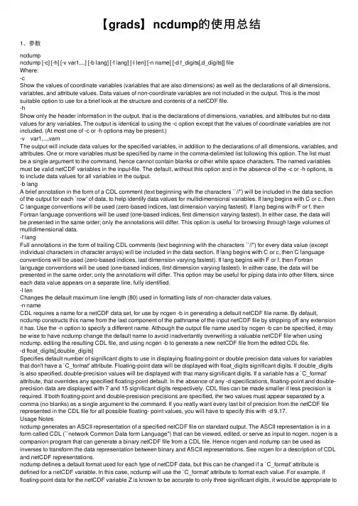
【grads】ncdump的使⽤总结1、参数ncdumpncdump [-c] [-h] [-v var1,...] [-b lang] [-f lang] [-l len] [-n name] [-d f_digits[,d_digits]] fileWhere:-cShow the values of coordinate variables (variables that are also dimensions) as well as the declarations of all dimensions, variables, and attribute values. Data values of non-coordinate variables are not included in the output. This is the most suitable option to use for a brief look at the structure and contents of a netCDF file.-hShow only the header information in the output, that is the declarations of dimensions, variables, and attributes but no data values for any variables. The output is identical to using the -c option except that the values of coordinate variables are not included. (At most one of -c or -h options may be present.)-v var1,...,varnThe output will include data values for the specified variables, in addition to the declarations of all dimensions, variables, and attributes. One or more variables must be specified by name in the comma-delimited list following this option. The list must be a single argument to the command, hence cannot contain blanks or other white space characters. The named variables must be valid netCDF variables in the input-file. The default, without this option and in the absence of the -c or -h options, is to include data values for all variables in the output.-b langA brief annotation in the form of a CDL comment (text beginning with the characters ``//'') will be included in the data section of the output for each `row' of data, to help identify data values for multidimensional variables. If lang begins with C or c, then C language conventions will be used (zero-based indices, last dimension varying fastest). If lang begins with F or f, then Fortran language conventions will be used (one-based indices, first dimension varying fastest). In either case, the data will be presented in the same order; only the annotations will differ. This option is useful for browsing through large volumes of multidimensional data.-f langFull annotations in the form of trailing CDL comments (text beginning with the characters ``//'') for every data value (except individual characters in character arrays) will be included in the data section. If lang begins with C or c, then C language conventions will be used (zero-based indices, last dimension varying fastest). If lang begins with F or f, then Fortran language conventions will be used (one-based indices, first dimension varying fastest). In either case, the data will be presented in the same order; only the annotations will differ. This option may be useful for piping data into other filters, since each data value appears on a separate line, fully identified.-l lenChanges the default maximum line length (80) used in formatting lists of non-character data values.-n nameCDL requires a name for a netCDF data set, for use by ncgen -b in generating a default netCDF file name. By default, ncdump constructs this name from the last component of the pathname of the input netCDF file by stripping off any extension it has. Use the -n option to specify a different name. Although the output file name used by ncgen -b can be specified, it may be wise to have ncdump change the default name to avoid inadvertantly overwriting a valuable netCDF file when using ncdump, editing the resulting CDL file, and using ncgen -b to generate a new netCDF file from the edited CDL file.-d float_digits[,double_digits]Specifies default number of significant digits to use in displaying floating-point or double precision data values for variables that don't have a `C_format' attribute. Floating-point data will be displayed with float_digits significant digits. If double_digits is also specified, double-precision values will be displayed with that many significant digits. If a variable has a `C_format' attribute, that overrides any specified floating-point default. In the absence of any -d specifications, floating-point and double-precision data are displayed with 7 and 15 significant digits respectively. CDL files can be made smaller if less precision is required. If both floating-point and double-presision precisions are specified, the two values must appear separated by a comma (no blanks) as a single argument to the command. If you really want every last bit of precision from the netCDF file represented in the CDL file for all possible floating- point values, you will have to specify this with -d 9,17.Usage Notesncdump generates an ASCII representation of a specified netCDF file on standard output. The ASCII representation is in a form called CDL (``network Common Data form Language'') that can be viewed, edited, or serve as input to ncgen. ncgen is a companion program that can generate a binary netCDF file from a CDL file. Hence ncgen and ncdump can be used as inverses to transform the data representation between binary and ASCII representations. See ncgen for a description of CDL and netCDF representations.ncdump defines a default format used for each type of netCDF data, but this can be changed if a `C_format' attribute is defined for a netCDF variable. In this case, ncdump will use the `C_format' attribute to format each value. For example, if floating-point data for the netCDF variable Z is known to be accurate to only three significant digits, it would be appropriate touse the variable attributeZ:C_format = "%.3g"ncdump may also be used as a simple browser for netCDF data files, to display the dimension names and sizes; variable names, types, and shapes; attribute names and values; and optionally, the values of data for all variables or selected variables in a netCDF file.ExamplesLook at the structure of the data in the netCDF file foo.nc:ncdump -c foo.ncProduce an annotated CDL version of the structure and data in the netCDF file foo.nc, using C-style indexing for the annotations:ncdump -b c foo.nc > foo.cdlOutput data for only the variables uwind and vwind from the netCDF file foo.nc, and show the floating-point data with only three significant digits of precision:ncdump -v uwind,vwind -d 3 foo.ncProduce a fully-annotated (one data value per line) listing of the data for the variable omega, using Fortran conventions for indices, and changing the netCDF dataset name in the resulting CDL file to omega:ncdump -v omega -f fortran -n omega foo.nc > Z.cdl2、注意①它是在dos底下⽤的，如果在gradsnc中⽤，请在命令前加感叹号。

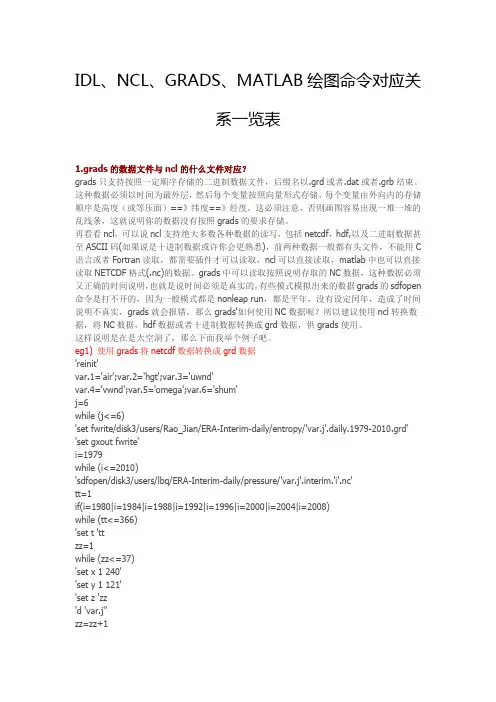
IDL、NCL、GRADS、MATLAB绘图命令对应关系一览表1.grads的数据文件与ncl的什么文件对应？grads只支持按照一定顺序存储的二进制数据文件，后缀名以.grd或者.dat或者.grb结束。

这种数据必须以时间为最外层，然后每个变量按照向量形式存储，每个变量由外向内的存储顺序是高度（或等压面）==》纬度==》经度。

这必须注意，否则画图容易出现一堆一堆的乱线条，这就说明你的数据没有按照grads的要求存储。

再看看ncl，可以说ncl支持绝大多数各种数据的读写，包括netcdf，hdf,以及二进制数据甚至ASCII码(如果说是十进制数据或许你会更熟悉)，前两种数据一般都有头文件，不能用C 语言或者Fortran读取，都需要插件才可以读取，ncl可以直接读取，matlab中也可以直接读取NETCDF格式(.nc)的数据。

grads中可以读取按照说明存取的NC数据，这种数据必须又正确的时间说明，也就是说时间必须是真实的，有些模式模拟出来的数据grads的sdfopen 命令是打不开的，因为一般模式都是nonleap run，都是平年，没有设定闰年，造成了时间说明不真实，grads就会报错。

那么grads'如何使用NC数据呢？所以建议使用ncl转换数据，将NC数据，hdf数据或者十进制数据转换成grd数据，供grads使用。

这样说明是在是太空洞了，那么下面我举个例子吧。

eg1) 使用grads将netcdf数据转换成grd数据'reinit'var.1='air';var.2='hgt';var.3='uwnd'var.4='vwnd';var.5='omega';var.6='shum'j=6while (j<=6)'set fwrite/disk3/users/Rao_Jian/ERA-Interim-daily/entropy/'var.j'.daily.1979-2010.grd' 'set gxout fwrite'i=1979while (i<=2010)'sdfopen/disk3/users/lbq/ERA-Interim-daily/pressure/'var.j'.interim.'i'.nc'tt=1if(i=1980|i=1984|i=1988|i=1992|i=1996|i=2000|i=2004|i=2008)while (tt<=366)'set t 'ttzz=1while (zz<=37)'set x 1 240''set y 1 121''set z 'zz'd 'var.j''zz=zz+1endwhilett=tt+1endwhileelsewhile (tt<=365)'set t 'ttzz=1zz=1while (zz<=37)'set x 1 240''set y 1 121''set z 'zz'd 'var.j''zz=zz+1endwhilett=tt+1endwhileendifi=i+1name='/disk3/users/lbq/ERA-Interim-daily/pressure/'var.j'.interim.'i'.nc''close 1'endwhile'disable fwrite'j=j+1endwhileeg2)使用ncl将数据输出成二进制数据，grads可以使用(截取部分)patho = "/disk3/users/Rao_Jian/Hadley/"system("rm "+patho+"ev_ts.grd")system("rm "+patho+"ev_ts2.grd")system("rm "+patho+"ev_ts.txt")system("rm"+patho+"ev_ts2.txt")do nt=0,719fbindirwrite(patho+"ev_ts.grd",ev_ts(:,nt));写成二进制数据，供grads使用end dofbindirwrite(patho+"ev_ts2.grd",ev_ts(time|:,evn|:))asciiwrite(patho+"ev_ts.txt",ev_ts(time|:,evn|:))；写成十进制数据，可以贴到EXCEL中使用asciiwrite(patho+"ev_ts2.txt",ev_ts);print(ev_ts(0,:))此外ncl中还有其他的读写函数，如fbinrecread,fbinrecwrite,fbinwrite,fbinreadncl读取netcdf3/4、hdf4、grib-1/2也是通过文件操作的eg3)ncl支持直接读取格式文件的读法fi = addfile(pathi+"HadISST_sst.nc","r")sst0 =fi->sst(960:1679,:,:) ; load 50 year data duringfrom 1950 to 2009注意：这类文件的后缀名一般为.nc /.hdf/ .grb/.hdfeos/.ccm2.grads中的描述文件与ncl中的什么对应描述文件（.ctl)是一个纯文本文件，我们有数据grads还是不能出图，需要一个描述文件来指定他的存储数据个数，维度（时间长度、层数和经纬度信息）。

GrADS绘图软件实用手册2002年1月目录第一章GrADS绘图软件概述1.GrADS绘图软件简介2.Internet上的GrADS资源2.1GrADS在Internet上的主页2.2windows环境下GrADS资源3.GrADS绘图软件的安装（windows环境）3.1在windows环境下安装GrADS软件包X server 的安装第二章GrADS绘图模板1.GrADS示例演示1.1 启动GrADS1.2 退出GrADS1.3 示例演示GrADS命令的使用2.GrADS绘图模板3.GrADS模板的高级应用GrADS描述语言GrADS高级模板的应用第三章GrADS数据格式1.格点数据描述文件1.1 数据描述文件各项解释1.2 生成model.le.dat和model.le.ctl文件的程序代码片段2.站点数据的格式附录1.如何精确控制图形输出的尺寸—Landscape纸型2.台站资料的显示3.Linux环境下的安装第二章GrADS绘图软件概述1GrADS绘图软件简介The Grid Analysis and Display System(GrADS) 是一套应用广泛、使用方便的科学数据绘图软件包。

其主要特点：●GrADS属于自由软件，可以从Internet上免费获得。

●可运行于各种Windows 和Unix工作平台。

●GrADS可用于4D数据的分析。

既经度、纬度、层（气压层、高度层等）和时间/xyzt 4维。

数据可以是格点化的数据或离散点数据。

GrADS特别适用于气象类数据的分析。

但也完全可以用于更广泛类型的数据分析。

●GrADS有多种显示方式：等值线、流线、矢量图、风矢量图、站点填图、折线图、直方图等多种两维图形。

●可处理多种数据格式的数据。

GRIB、NetCDF、HDF-SDS等通用数据格式和系统自定义的一种二进制数据格式。

●采用命令行输入的方式交互式地显示图形。

并有多种命令对数据进行再加工。

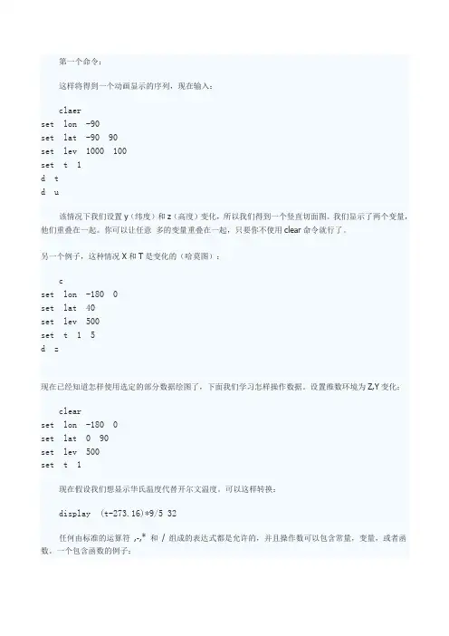
第一个命令：这样将得到一个动画显示的序列，现在输入：claerset lon -90set lat -90 90set lev 1000 100set t 1d td u该情况下我们设置y（纬度）和z（高度）变化，所以我们得到一个竖直切面图。

我们显示了两个变量，他们重叠在一起。

你可以让任意多的变量重叠在一起，只要你不使用clear命令就行了。

另一个例子，这种情况X和T是变化的（哈莫图）：cset lon -180 0set lat 40set lev 500set t 1 5d z现在已经知道怎样使用选定的部分数据绘图了，下面我们学习怎样操作数据。

设置维数环境为Z,Y变化：clearset lon -180 0set lat 0 90set lev 500set t 1现在假设我们想显示华氏温度代替开尔文温度。

可以这样转换：display (t-273.16)*9/5 32任何由标准的运算符,-,* 和/ 组成的表达式都是允许的，并且操作数可以包含常量，变量，或者函数。

一个包含函数的例子：d sqrt(u*u v*v)有一个函数用来计算风的级数。

d mag(u,v)另一个内建函数计算平均值：clear d ave(a,t=1,t=5)这种情况我们可以计算5天的平均。

我们也可以从数据中移除平均值（距平值）：d z-ave(z,t=1,t=5)也可以在x方向作平均并求距平：cleard z-ave(z,x=1,x=72)也可以做时间差分：cleard z(t=2)-z(t=1)完整规范的变量名是：name.file(dim |-|=va lue,…) 如果我们打开了两个文件，也许一个是模式输出，另一个是分析，我们应该区分用如下方法二者：display z.2-z.1另一个内置的函数通过有线差分计算水平涡度相关cleard hcurl(u,v)还有另外一个计算数值方向的质量积分：cleard vint(ps,q,275)这儿我们计算了可降水量（单位mm）现在来讨论控制图形输出的话题。

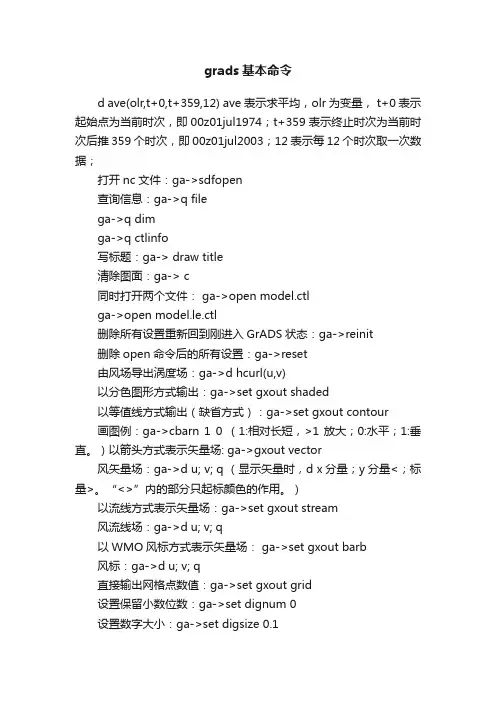
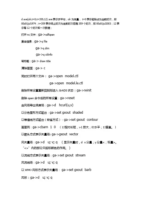
grads基本命令d ave(olr,t+0,t+359,12) ave表示求平均，olr 为变量， t+0表示起始点为当前时次，即00z01jul1974；t+359表示终止时次为当前时次后推359个时次，即00z01jul2003；12表示每12个时次取一次数据；打开nc文件：ga->sdfopen查询信息：ga->q filega->q dimga->q ctlinfo写标题：ga-> draw title清除图面：ga-> c同时打开两个文件： ga->open model.ctlga->open model.le.ctl删除所有设置重新回到刚进入GrADS状态：ga->reinit删除open命令后的所有设置：ga->reset由风场导出涡度场：ga->d hcurl(u,v)以分色图形方式输出：ga->set gxout shaded以等值线方式输出（缺省方式）：ga->set gxout contour画图例：ga->cbarn 1 0 （1:相对长短，>1放大；0:水平；1:垂直。

）以箭头方式表示矢量场: ga->gxout vector风矢量场：ga->d u; v; q （显示矢量时，d x分量；y分量<；标量>。

“<>”内的部分只起标颜色的作用。

）以流线方式表示矢量场：ga->set gxout stream风流线场：ga->d u; v; q以WMO风标方式表示矢量场： ga->set gxout barb风标：ga->d u; v; q直接输出网格点数值：ga->set gxout grid设置保留小数位数：ga->set dignum 0设置数字大小：ga->set digsize 0.1ga->set mpdraw on 如为off，不画地图背景（非经纬度数据需此项）ga->set poli on 如为off不画国界省界等。

d ave(olr,t+0,t+359,12) ave表示求平均，olr 为变量， t+0表示起始点为当前时次，即00z01jul1974；t+359表示终止时次为当前时次后推359个时次，即00z01jul2003；12表示每12个时次取一次数据；打开nc文件：ga->sdfopen查询信息：ga->q filega->q dimga->q ctlinfo写标题：ga-> draw title清除图面：ga-> c同时打开两个文件： ga->open model.ctlga->open model.le.ctl删除所有设置重新回到刚进入GrADS状态：ga->reinit删除open命令后的所有设置：ga->reset由风场导出涡度场：ga->d hcurl(u,v)以分色图形方式输出：ga->set gxout shaded以等值线方式输出（缺省方式）：ga->set gxout contour画图例：ga->cbarn 1 0 （1:相对长短，>1放大；0:水平；1:垂直。

）以箭头方式表示矢量场: ga->gxout vector风矢量场：ga->d u; v; q （显示矢量时，d x分量；y分量<；标量>。

“<>”内的部分只起标颜色的作用。

）以流线方式表示矢量场：ga->set gxout stream风流线场：ga->d u; v; q以WMO风标方式表示矢量场： ga->set gxout barb风标：ga->d u; v; q直接输出网格点数值：ga->set gxout grid设置保留小数位数：ga->set dignum 0设置数字大小：ga->set digsize 0.1ga->set mpdraw on 如为off，不画地图背景（非经纬度数据需此项）ga->set poli on 如为off不画国界省界等。

第一个命令：这样将得到一个动画显示的序列，现在输入：claerset lon -90set lat -90 90set lev 1000 100set t 1d td u该情况下我们设置y（纬度）和z（高度）变化，所以我们得到一个竖直切面图。

我们显示了两个变量，他们重叠在一起。

你可以让任意多的变量重叠在一起，只要你不使用clear命令就行了。

另一个例子，这种情况X和T是变化的（哈莫图）：cset lon -180 0set lat 40set lev 500set t 1 5d z现在已经知道怎样使用选定的部分数据绘图了，下面我们学习怎样操作数据。

设置维数环境为Z,Y变化：clearset lon -180 0set lat 0 90set lev 500set t 1现在假设我们想显示华氏温度代替开尔文温度。

可以这样转换：display (t-273.16)*9/5 32任何由标准的运算符,-,* 和/ 组成的表达式都是允许的，并且操作数可以包含常量，变量，或者函数。

一个包含函数的例子：d sqrt(u*u v*v)有一个函数用来计算风的级数。

d mag(u,v)另一个内建函数计算平均值：clear d ave(a,t=1,t=5)这种情况我们可以计算5天的平均。

我们也可以从数据中移除平均值（距平值）：d z-ave(z,t=1,t=5)也可以在x方向作平均并求距平：cleard z-ave(z,x=1,x=72)也可以做时间差分：cleard z(t=2)-z(t=1)完整规范的变量名是：name.file(dim |-|=va lue,…) 如果我们打开了两个文件，也许一个是模式输出，另一个是分析，我们应该区分用如下方法二者：display z.2-z.1另一个内置的函数通过有线差分计算水平涡度相关cleard hcurl(u,v)还有另外一个计算数值方向的质量积分：cleard vint(ps,q,275)这儿我们计算了可降水量（单位mm）现在来讨论控制图形输出的话题。

1.ctl文件的编写dset d:\test\test1.dat 数据文件路径名和文件名title monthly precipitation data 数据标题options 365_day_calendar 特殊格式说明365_day_calendar/template(多个文件) undef -9999.0 缺测值，若有多个则用fortran改写成同一个缺测值xdef 144 linear 0 2.5 x维数格点数/排列方式/起始值/间隔*linear线性/levels列举ydef 73 linear -90 2.5 y维数zdef 5 linear 1000 850 700 500 200 z维数tdef 24 linear 00z01Jan1979 1mo 时间维数*mo月yr年vars 1 变量数precip 1 99 *precipitation data 变量名/层数/排列顺序/说明endvars*变量循环顺序：x经度y维度z高度v变量t时间*注释行第一列用‘*’，注释行不能出现在变量列表中2.维数环境设置set lon/lat/lev/time var1 <var2> *实际值set x/y/z/t var1 <var2> *格点数值*两种坐标可以混用3.图形文件的保存gxprint/printim **.png/jpg/pdf/eps…. whiteenable print **.gmfprintdisableprint4.图形类型的设置set gxout typecontour 二位等值线图*默认shaded 二维填色等值线图vector 矢量箭头二维风场图*d u;v时为默认bar 直方图line 折线图*默认…………………5.图形要素设置gxout=contour or shadedset cint value 设置等值线间隔set clevs lev1,lev2,……设置特定等值线set ccols col1,col2,……设置对应于set clevs的等值线的颜色cbarn size 0/1 x y 设置色标gxout=line or contourset ccolor color 设置线条颜色set cstyle style设置线条样式1实线2长虚线3短虚线……set cthick thickns 设置线条粗细1~10set cmark marker 设置数据点标记0无标记*line时有效gxout=barset bargap val 设置直方条间隔*0~100百分比，0为无间隔set barbase val/bottom/top 设置直方条起始值gxout=vectorset arrscl size <magnitude> 设置箭头长度set arrowhead size 设置箭头大小，缺省为0.056.gs文件的编写将命令用单引号括起来7.变量define varname=expression 定义变量‘d air(t=3)’‘d air(t=3,z=5)’‘d air(lev=1000)-air(lev=500)’设置变量维数8.平均函数ave(expr,dimexpr1,dimexpr2,<timeint>) 一维平均aave(expr,dimexpr1,dimexpr2, dimexpr3,dimexpr4,) 二维平均*不能对z、t *需将维度设置成点9.地图投影设置set mproj proj 设置地图投影方式latlon 缺省nps 北半球极地投影sps 南半球极地投影set map color style thickness 设置背景地图线条颜色、线型、宽度10.绘图区域设置set parea xmin xmax ymin ymax11.坐标要素控制set frame on/off/circle 绘制图形边框/不绘制/绘制圆形边框set grads on/off 标记grads及绘图时间draw title <string> 绘制标题draw xlab/ylab <string> 绘制x轴/y轴图注set xyrev on/off xy轴互换set zlog on/off z方向用对数坐标set xlint/ylint value 设置x/y轴坐标刻度间隔set vrange val1 val2 设置y轴范围set vrange2 val1 val2 设置x轴范围set xlopts/ylopts color thickness size x/y轴刻度值的颜色、线宽、大小*缺省1,4,0.12 set tlsupp year 去掉年份显示12.颜色的定义‘define_colors’使用内部默认颜色标号13.基本绘图命令set line color style thickness 设置颜色、线型、线宽draw line x1 y1 x2 y2 绘制直线draw rec/recf x1 y1 x2 y2 绘制不填色/填色矩形draw mark type x y size 绘制标记*1叉2空心圆3实心圆4空心方框5实心方框draw string x y string 绘制字符串set strsiz hsiz <vsiz> 设置字符大小14.文件操作(1)输出二进制变量设置维数环境‘set gxout fwrite’‘set fwrite ***.dat’‘d var’(2)读写有格式文件result=read(filename)result 第一行：返回码（0 OK，1打开错误2文件结束8文件状态为写入9I/O错误）result 第二行：读取的文件内容Text = sublin(result,2) 将result相应行的内容赋值给Textaa=subwrd(Text,#n) 将Text的第n个值赋值给aaresult=write(filename, text, <append>)15.维数查询q w2xy lon lat 将经纬度坐标转换为图形窗口坐标返回值：X=*** Y=*** q xy2w X Y 将图形窗口坐标转为经纬度坐标返回值：Lon=*** Lat=***q w2gr lon lat 将经纬度坐标转换为格点坐标返回值：Xdim=*** Ydim=***q gr2w xdim ydim 将格点坐标转换为经纬度坐标返回值：Lon=*** Lat=***q xy2gr X Y 将图形窗口坐标转换为格点坐标返回值：Xdim=*** Ydim=***q gr2xy xdim ydim 将格点坐标转换为经纬度坐标返回值：X=*** Y=***16.气候平均设置季节变量‘set t 1 12’‘define climate=ave(var,t+0,t=tmax,12)’‘modify climate seasonal’滑动平均‘set t 1 tmax’‘define running_mean=ave(var,t-n,t+n)’17.站点资料绘图(1)转换生成数据文件及格点文件数据文件的顺序为先循环站号再循环时间，每条记录包含站号-纬度-经度-时间-nlev-flag-数据，每循环完一个时间后要加一个不写数据且nlev=0的记录(2)编写ctldtype stationstnmap ***.map**变量层数为0(3)生成.map映射文件!stnmap –i */*/*.ctl(4)插值‘open ***\grid.ctl’‘open ***dat.ctl’‘define varname=oacres(grid,var.2)’(5)绘图‘cnbasemap varname’18.绘制路径图。

所有指令介绍13.1常用指令及无联锁指令在运行过程中执行动作动作注释地址范围事指令地址位置时间常数件N Q,I,M,D*M.N当前步激活时，信0.0-65535.7号置1，步失效时置0。

（无关互锁）步激活时，信号置1 S Q,I,M,D*M.N并保持置1，直到下0.0-65535.7次复位（无关互锁）R Q,I,M,D*M.N步激活时，信号值0.0-65535.70，并保持。

（无关互锁）0.0-65535.7D Q,I,M,D*M.N T#<const>当前步激活，延迟T#TIME时间后置1，当前步激活时间小于T#TIME则不置1，当前步失效后置复位。

（无关互锁）步激活时，信号值L Q,I,M,D* M.NT#<const> 当前步激活时，持 续 T#TIME 时间置1，时间过后置 0，当前步失效后复 位。

（无关互锁）0.0-65535.7CALLFB,FC,SFB,S FCBlock nu m ber只要当前步激活，就调用其他功能块。

（无关互锁）NC Q,I,M,D* M.N 当前步激活时，在0.0-65535.7满足互锁条件下， 信号置 1，不满足互 锁条件下置 0。

当前 步失效后复位。

步激活时，在满足 互锁条件下，信号 SC Q,I,M,D* M.N0.0-65535.7置 1 并保持置 1，直 到下次复位.RC Q,I,M,D* M.N0.0-65535.70，并保持。

（无关互锁）DCQ,I,M,D*M.NT#<const> 当前步激活，延迟T#TIME 时间后置1，当前步激活时间小于 T#TIME 则不 置 1，当前步失效后 置复位。

（无关互 锁）LCQ,I,M,D*M.NT#<const> 当前步激活时，持续 T#TIME 时间置 1，时间过后置 0，当前步失效后复 位。

（无关互锁）0.0-65535.70.0-65535.7CALLCFB,FC,SFB,S FCBlock nu m ber只要当前步激活，就调用其他功能顺控器 FB 块引脚参数说明：FB 参数（上升沿有效） 内部变量（静态数据区名称） 块。

GrADS 精致绘图说（一）1. basemap.gs:basemap L | O | U <fill_color> <out_color> <hi/lo>在低分辨率海岸廓线范围内用颜色覆盖陆地／海洋。

适用于各种投影方式，需lpoly.asc, lpoly_hires.asc, lpoly_US.asc, opoly.asc, opoly_hires.asc文件。

其中：L(l)：覆盖陆地，O(o)：覆盖海洋，U(u)：覆盖20N-50N的墨西哥和加拿大领土（低分辨率，适用美国），fill_color：填充色号，缺省为15，out_color：廓线的颜色号，缺省为15，hi/lo：高分辨率('set mpdset hires'，仅对15N-53N, 130W-60W区域)/低分辨率。

2. cbar.gs、cbarn.gs、cbarc.gs、cbar_l.gs和cbar_line.gs:cbarn sf vert xmid ymidcbarc center_x center_y back_color绘制'set gxout shaded'图形的填色标尺。

sf：色标尺寸，1为全尺寸，0.5为半尺寸；vert：0为水平，1为垂直；xmid,ymid：色标中心点的位置。

cbar_l -x X -y Y -n number -t text -pcbar_line -x X -y Y -c color -m mark -l linestyle -t text -p加'set gxout line'的图例说明。

其中：-x,-y：图中x和y的位置，-n：线条的数目（最多可为10条），-t：文字说明的内容（最多10条，需双引号括起），-c：线和标记的颜色，-m：定义标记；-l：定义线型，-p：用户可在图中点击给定图例的放置位置。

3. colors.gs:为雪盖(颜色序号40~45)、降水(颜色序号50~59)及温度(颜色序号64~85)资料的shaded图设置填充色。

几个有用的GRADS函数monmask多年时间序列中显示每年的相同月的资料<run> monmask.gs 5 define mmask for May (5)d (expr)*mmask plot (expr) only for Maycbar_line: 显示图例exp: cbar_line -x num(x方向位置) -y num(y方向位置) -c num(线条颜色) -l num(线条类型) -n num(线条数，max=10) -m num(标记) -t "(文本)" -p (加上-p，就不要-x, -y, 鼠标点到哪里就画在那)cbar: 对shaded图形有效，做图例cbarn: 同上，可加参数，exp: cbarn 1(图例粗细) 1(图例竖放，横放=0) <5(图例位置，x方向)> <5(图例位置，y方向)>cbarc: 同上，默认图例在右上角，可加参数，exp: cbarc <5(图例位置，x方向)> <5(图例位置，y方向)>connect_the_dots: 用鼠标画线，点击图的下方退出，无参数font: 设置字体，参数0-5，默认font=0, ROMAN字体为font=1loop: 循环作图，exp: loop x(or y，z，t，lat，lon，lev) min(起始值) max(最终值) step(步长)page: 选择画图区域，usage:run page top plot on top half of screenrun page bottom plot on bottom half of screenrun page left plot on left half of screenrun page right plot on right half of screenrun page q1 plot on quadrent 1run page q2 plot on quadrent 2run page q3 plot on quadrent 3run page q4 plot on quadrent 4run page xy XY (x,y,X,Y) are single digitsxy = location, XY = sizeonly 1 blank between xy and XYquadrents:-----------| q1 | q2 |-----------| q3 | q4 |-----------Matrix notation:xy is the location of the pageXY is number of subdivisionsThe idea here is that the page is divided into a grid of X by Yrectangles. Plotting is done in the x-y rectangle. In thefollowing example, the page is divided into two columns (X=2)and 3 rows (Y=2).-----------| 13 | 23 |-----------| 12 | 22 | xy values for XY=23-----------| 11 | 21 |-----------To draw into the top left rectangle, you "run page 13 23".To get the bottom right rectangle, you "run page 21 23".The following commands are equivalennt:"run page q1" "run page 12 22""run page q2" "run page 22 22""run page top" "run page 12 12""run page bottom" "run page 11 12"Limitations: X and Y must have values from 1 to 9.关掉多图形显示：page offsave: 保存图形，exp: save <路径>文件名.gmfwrdlin: 用经纬度画直线，exp: wrdlin minlon(起始经度) minlat(起始纬度) maxlon(最后经度) maxlat(最后纬度)wrdmrk: 在经纬度上标记，exp: wrdmrk num(标记类型) lon(经度) lat(纬度) siz(大小)wrdrec: 在图上画矩形，exp: wrdrec minlon(起始经度) minlat(起始纬度)[矩形左下角坐标] maxlon(最后经度) maxlat(最后纬度)[矩形右上角坐标]wrdrecf: 掩盖矩形内的图形，exp: wrdrec minlon(起始经度) minlat(起始纬度)[矩形左下角坐标] maxlon(最后经度) maxlat(最后纬度)[矩形右上角坐标]wrdstr: 在图上写字符串，exp: wrdstr lon(经度) lat(纬度) "(字符串)"map: 设置地图投影，nps (north-pole stereographic) lat='20 90' lon='-270 90'nps2 (north-pole stereographic) lat='20 90' lon='-180 180'nps3 (north-pole stereographic) lat='20 90' lon='-60 300'sps (sorth-pole stereographic) lat='-90 -20' lon='-270 90'lola (lat-lon) (0..360)'lola2 (lat-lon) (-180..180)'usa 'latlon' lat='24 52' lon='-127 -65'usa2 'nps' lat='15 80' lon='-150 -45'n_amer 'nps' lat='5 90' lon='-270 90's_amer 'latlon' lat='-60 20' lon='-90 -30'africa 'latlon' lat='-40 50' lon='-20 60'europe 'nps' lat='5 90' lon='-180 180'euro2 'nps' lat='5 90' lon='-180 180'asia 'latlon' lat='0 80' lon='40 170'aust 'latlon' lat='-50 0' lon='100 180'robinson 'robinson' lat='-90 90' lon='-180 180'c_pac 'latlon' lat='-45 45' lon='120 290'n_pac 'nps' lat='0 90' lon='90 270'custom [lon0 dlon lat0 dlat] (lat0,lon0=left-bottom corner)。