DSC-TGA谱图综合解析教学文稿
- 格式:ppt
- 大小:1.94 MB
- 文档页数:36

综合同步热分析(T G A-D S C)实验讲义一、实验目的:用热分析仪对进行TG和DSC分析,并对热分析谱图进行定性和定量分析。
二、预习要求1、了解热分析仪的工作原理和操作方法;2、了解TG和DSC分析的基本原理及热分析谱图的意义。
三、原理1、热分析的定义:热分析(thermal analysis):顾名思义,可以解释为以热进行分析的一种方法。
1977年在日本京都召开的国际热分析协会(ICTA)第七次会议上,给热分析下了如下定义:即热分析是在程序控制温度下,测量物质的物理、化学性质与温度的关系的一类技术。
通俗来说,热分析是通过测定物质加热或冷却过程中物理性质(目前主要是重量和能量)的变化来研究物质性质及其变化,或者对物质进行分析鉴别的一种技术。
程序控制温度:一般是指线性升温或线性降温,当然也包括恒温、循环或非线性升温、降温。
也就是把温度看作是时间的函数:T=φ(t); t:时间。
常见的物理变化:熔化、沸腾、升华、结晶转变等;常见的化学变化:脱水、降解、分解、氧化,还原、化合反应等。
这两类变化,常伴有焓变,质量、机械性能和力学性能等的变化。
2、热分析存在的客观物质基础在目前热分析可以达到的温度范围内,从-150℃到1500℃(或2400℃),任何两种物质的所有物理、化学性质是不会完全相同的。
因此,热分析的各种曲线具有物质“指纹图”的性质。
3、热分析的起源及发展1899 年英国罗伯特-奥斯汀(Roberts-Austen)第一次使用了差示热电偶和参比物,大大提高了测定的灵敏度,正式发明了差热分析(DTA)技术。
1915 年日本东北大学本多光太郎,在分析天平的基础上研制了“热天平”即热重法(TG),后来法国人也研制了热天平技术。
1964 年美国瓦特逊(Watson)和奥尼尔(O’Neill)在DTA技术的基础上发明了差示扫描量热法(DSC)。
美国P-E公司最先生产了差示扫描量热仪,为热分析热量的定量作出了贡献。
热重分析仪T G A—D S C 本页仅作为文档封面,使用时可以删除This document is for reference only-rar21year.March什么是热分析热分析是在程序温度(指等速升温、等速降温、恒温或等级升温等)控制下测量物质的物理性质随温度的变化,用于研究物质在某一特定温度时所发生的热学、力学、声学、光学、电学、磁学等物理参数的变化。
由此进一步研究物质的结构和性能。
热重法:在程序温度控制下测量试样的质量随温度变化的一种技术。
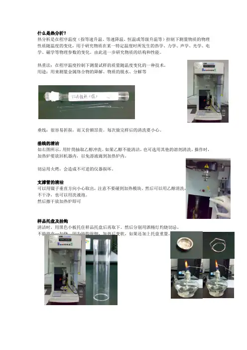
用途:用来测量金属络合物的降解、物质的脱水、分解等垂线:很容易折损,而又价额昂贵。
每次做完样后的清洗要小心。
垂线的清洁如右图所示,用针筒抽取乙醇冲洗。
如果乙醇不能清洁,也可选用其他的溶剂清洗。
操作时,加热炉要放回机器内,以免溶液滴到加热炉内。
切忌用火烤,会造成不可逆的仪器损坏。
支撑管的清洁可以用镊子垂直方向小心取出,注意不要碰到加热模块。
然后可以用乙醇清洗,如果还是擦不干净,也可以用洗液泡。
然后擦干放加热炉即可样品托盘及挂钩清洁时,用黑色小板托住样品托盘后再取下。
然后分别用酒精灯灼烧切忌,不能放在一起烧,因为挂钩很细,加热后变软,如果还加上托盘重量,就很容易变形。
TGA图怎么看TGA 举例1:取点规则,一般在平台的两边。
失重线,纵坐标为重量剩余百分比。
微分线,由失重线的失重速度快慢所得到,即如有特殊报告要求,也可以选△Y ,△X ,Onset 等。
横坐标也可以是时间,如果这时作微分线,那微分线得意思就是△W/△Time 80℃-120℃左右,一般为游离水的失重造成TGA举例2TGA举例3这个失重的开时温度比前一个要早一些。
推测它的失重是由水或某种有机溶剂的残留引起30℃-60℃可能是因为有机溶剂引起的失重,列入乙醇等。
150℃和300℃是样品的分部分解引起的TGA举例4TGA举例5一般失重总在0%-100%之间,但也有例外的情况。
这个样品有升华现象,并且结晶凝在支撑管和托盘之间,这时的称重就不再是样品称重,这个图就达到了-20%有些溶剂(多为有机溶剂),在初始温度时就不断失重,恒温很久也得不到恒定重量,这样就不能测准易挥发物的含量。
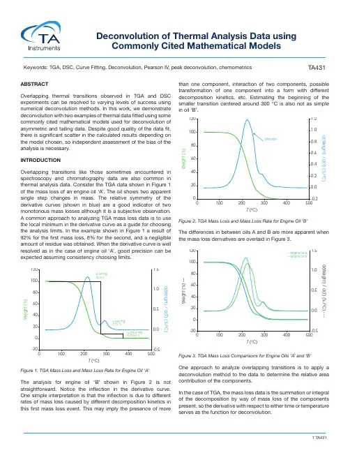
TA431Deconvolution of Thermal Analysis Data usingCommonly Cited Mathematical ModelsKeywords: TGA, DSC, Curve Fitting, Deconvolution, Pearson IV , peak deconvolution, chemometrics ABSTRACTOverlapping thermal transitions observed in TGA and DSC experiments can be resolved to varying levels of success using numerical deconvolution methods. In this work, we demonstrate deconvolution with two examples of thermal data fitted using somecommonly cited mathematical models used for deconvolution of asymmetric and tailing data. Despite good quality of the data fit, there is significant scatter in the calculated results depending onthe model chosen, so independent assessment of the bias of theanalysis is necessary.INTRODUCTIONOverlapping transitions like those sometimes encountered inspectroscopy and chromatography data are also common inthermal analysis data. Consider the TGA data shown in Figure 1 of the mass loss of an engine oil ‘A’. The oil shows two apparentsingle step changes in mass. The relative symmetry of the derivative curves (shown in blue) are a good indicator of twomonotonous mass losses although it is a subjective observation.A common approach to analyzing TGA mass loss data is to usethe local minimum in the derivative curve as a guide for choosingthe analysis limits. In the example shown in Figure 1 a result of 92% for the first mass loss, 8% for the second, and a negligible amount of residue was obtained. When the derivative curve is wellresolved as in the case of engine oil ‘A’, good precision can be expected assuming consistency choosing limits.Figure 1. TGA Mass Loss and Mass Loss Rate for Engine Oil ‘A’The analysis for engine oil ‘B’ shown in Figure 2 is not straightforward. Notice the inflection in the derivative curve.One simple interpretation is that the inflection is due to differentrates of mass loss caused by different decomposition kinetics inthis first mass loss event. This may imply the presence of morethan one component, interaction of two components, possible transformation of one component into a form with differentdecomposition kinetics, etc. Estimating the beginning of the smaller transition centered around 300 °C is also not as simple in oil ‘B’. Figure 2. TGA Mass Loss and Mass Loss Rate for Engine Oil ‘B’The differences in between oils A and B are more apparent when the mass loss derivatives are overlaid in Figure 3.Figure 3. TGA Mass Loss Comparisons for Engine Oils ‘A’ and ‘B’One approach to analyze overlapping transitions is to apply a deconvolution method to the data to determine the relative areacontribution of the components. In the case of TGA, the mass loss data is the summation or integralof the decomposition by way of mass loss of the componentspresent, so the derivative with respect to either time or temperatureserves as the function for deconvolution.W e i g h t (%)T (ºC)d(Weight) / d(T ) (%/ºC)120 1.51.00.50.0-0.5204060801000-2001002003004.69 mg 92.2 %0.392 mg 7.72 %4.20e-4 mg 8.27e-3 %400500W e i g h t (%)T (ºC)d(Weight) / d(T ) (%/ºC)W e i g h t (%) —T (ºC)d(Weight) / d(T ) (%/ºC) - - -120 1.51.00.00.5-0.5204060801000-200100200300— Engine Oil ‘A’— Engine Oil ‘B’400500In the case of DSC data, this is simply the heat flow curve which is a differential (Equation 1)(1)Where dq/dt is the differential heat flow rate, C P is the specific heat capacity, dT/dt is the heating rate (sometimes abbreviated as β), and f(T,t) are temperature and time dependent functions. A complication of deconvolution of DSC data is the possibility of simultaneous endothermic and exothermic transitions often prevalent in polymorphic transformations as an example. Careful evaluation of these potential kinetic dependent transitions should be undertaken before attempting any deconvolution. BACKGROUNDThe problem of resolving overlapping peaks is certainly not new. Asymmetry, significant fronting, and sometimes tailing often observed in thermal data results in distributions that are not modeled ideally with Gaussian or Lorentzian functions often used to deconvolve spectroscopic and chromatographic data. Several approaches have been published in the literature using functions that fit asymmetric data. Koga and coworkers [1] fit TGA data using 9 different mathematical functions including asymmetric double sigmoid, asymmetric logistic, extreme value 4 parameter fronted, Fraser-Suzuki, log normal 4 parameter, logistic power peak, Pearson I V , Pearson I V (a3 = 2), and Weibull with fitting criterion that r 2 > 0.99.Michael et al. developed a function for deconvolving DSC nickel titanium phase transformation heat flow data [2]. Deconvolution has been used to separate complex chemical processes for kinetic analysis shown in Figure 4 by Khachani et al. [3]Figure 4. Peak Deconvolution Using Frazer-Suzuki Function; β=7 °C/min [3]For this work, we fit examples using the following models: Pearson IV , Asymmetric Logistic, Extreme Value 4 Parameter Fronted, Log Normal 4 Area, Logistic Power Peak, and Exponentially Modified Gaussian (EMG).EXPERIMENTAL1. Example 1 – Comparison of Two Motor Oils a. Instrument – TA Instruments Discovery 5500 TGA b. Heating Rate 1 °C / min (modulated TGA Experiment)c. Crucible – Ptd. Purge – N 2 at 25 mL / mine. Sample Mass - 5 mg nominal 2. Example 2 – Dynamic Curing of Epoxya. Instrument – TA Instruments Discovery 2500 DSCb. Heating Rate - 10 °C / minc. Purge – N 2 at 50 mL / mind. Crucible – Tzero Aluminume. Sample Mass – 2 mg nominal DATA REDUCTIONTGA and DSC data were exported as text files and analyzed using PeakFit v4.12 (Systat). The models used for fitting the data are contained in the software. For conciseness, we show illustrated data only from the Pearson IV fit.RESULTS and DISCUSSION 1. Comparison of Two Motor Oilsa. Oil ‘A’ – Figure 5 (same data as Figure 1) shows a typical TGA data reduction for this sample. The limits chosen where based on the position of the relative minima of the derivative curves.Figure 5. TGA Mass Loss Data for Oil ‘A’Figure 6 shows the deconvolution of the derivative of mass loss with respect to temperature signal using the Pearson I V model. Other models and the resultant area fractions are summarized in Table 1dq dt= C p+ ƒ (T, t)dT dtd α/d t (m i n -1)Temperature (ºC)0,25Experimental reaction rate First ProcessSecond Process Total Process0,10,150,20,050110120130140150160170190200180W e i g h t (%)T (ºC)d(Weight) / d(T ) (%/ºC)120 1.51.00.50.0-0.5204060801000-2001002003004.66 mg 91.7 %0.420 mg 8.26 %4.20e-4 mg 8.27e-3 %400500Figure 6. Deconvolution of Derivative of Mass Loss for Oil ‘A’ Using Pearson IV ModelResiduals for Oil ‘A’ are shown in Figure 7Figure 7. Deconvolution Residuals for Oil ‘A’Table 1. Area % Calculations for Oil ‘A’ by ModelThe quality of the data fit using the models is good but in this case the results obtained using the using the derivative minimum as a guideline lie withing the scatter range of the results obtained using the models. This is explained by the relatively good separation of the mass loss events. The scatter of the data set is shown in Figure 8.Figure 8. Scatter of Peak 1 Data in Oil ‘A’ Deconvolutionb. Oil ‘B’ – Figure 9 (same data as Figure 2) shows the data reduction for this sample. As stated previously, the first mass loss does not appear to be monotonous and deconvolution should make improvements to more accurately analyze the data.Figure 9. TGA Mass Loss Data for Oil ‘B’Figure 10 shows the deconvolution of the derivative of mass losswith respect to temperature using the Pearson IV model.Pearson IV 89.3710.63 1.0000.0072Asymmetric Logistic 93.30 6.700.9970.0202Extreme Value 4 Area Fronted 91.128.8840.9990.0084Log Normal-4-Area90.829.179 1.0000.0079Logistic Power Peak93.38 6.6220.9970.0211Exponentially Modified Gaussian 92.067.940.9980.0154Derivative Minimum91.78.26--d W /d T (% / m i n )d W /d T (% / m i n )Temperature ºCdW/dT (% / min)dW/dT (% / min)R e s i d u a l sTemperature ºCResidualsA r e a %Data PointW e i g h t (%)T (ºC)d(Weight) / d(T ) (%/ºC)120 1.21.00.80.60.40.20.0-0.240608010020001002003001.65 mg 28.2 %3.67 mg 62.9 %0.513 mg 8.80 %6.03e-4 mg 0.0103 %400500Figure 10. Deconvolution of Derivative of M ass Loss for Oil ‘B’ Using Pearson IV ModelResiduals for Oil ‘B’ are shown in Figure x.Figure 11. Deconvolution Residuals for Oil ‘B’Table 2 compares area fraction differences in oil sample ‘B’ using the models and the derivative minimum method.Table 2. Area % Calculations for Oil ‘B’ by Modeld W /d T (% / ºC )d W /d T (% / ºC )Temperature ºCdW/dT (% / ºC)dW/dT (% / ºC)R e s i d u a l sTemperature ºCResidualsPearson IV 84.837.048.13 1.0000.0040Asymmetric Logistic 83.638.617.760.9990.0107Extreme Value 4 Area Fronted 79.167.5513.29 1.0000.0081Log Normal-4-Area82.25 6.1111.64 1.0000.0034Logistic Power Peak87.52 6.01 6.47 1.0000.0060ExponentiallyModified Gaussian 83.82 6.469.72 1.0000.0070Derivative Minimum62.928.28.80--In this case the quality of the data fit is also good and likely does improve the accuracy of the data relative to the derivative minimum. There is also significant scatter within the results obtained using the models and is shown in Figure 12.Figure 12. Scatter of Peak 1 Data in Oil ‘B’ Deconvolution2. DSC Evaluation of Epoxy Curing – This example shows two dynamic temperature ramps of a common epoxy. At time t 0, the DSC analysis is straightforward and is shown in Figure 13.Figure 13. Heat Flow of Epoxy Cure at Initial Time (t 0) at Heating Rate 10 °C / minAt time t as the epoxy cures, a second diffusion driven exothermictransition becomes apparent shown in Figure 14.A r e a %Data PointQ (m W )T (ºC)Exo Up2-11-202040608010012014069.3 ºC152.70 J/g 32.6 ºCFigure 14. Heat Flow of Epoxy Cure at Time (t) at Heating Rate 10 °C / minIn this case where the peaks are poorly resolved, deconvolution is a means to a more accurate value for the relative contribution of the reaction and diffusion heat flow. Deconvolution of the epoxy at time t shown in Figure 15 and residuals are shown in Figure 16.Figure 15. Deconvolution of Derivative of M ass Loss for Partially Cured Epoxy Using Pearson IV ModelFigure 16. Deconvolution Residuals for Partially Cured EpoxyTable 3 summarizes and compares the relative peak areas of the reaction and diffusion heat flow due to the curing of the epoxy.Q (W g )T (ºC)Exo UpH e a t F L o w (W /g )H e a t F l o w (W /g )Temperature ºCHeat FLow (W/g)Heat Flow (W/g)Table 3. Area % Calculations for Partially Cured Epoxy by ModelThe quality of the data fit using the models in this example is also good and likely approaches accurate results. We expect that the uncertainty in this particular example would be partially mitigated by choosing fit parameters for the reaction (1st exotherm) and diffusion exotherms (2nd exotherm) based on the apparent symmetry of the reaction exotherm at time t0 assuming that the corresponding reaction exotherm at time t (Figure 14) is similar.Despite the advantage of obtaining the t 0 data, the models yield significantly different values. Scatter of the first peak of the epoxy data is shown in Figure 17. The choice of the initial fitting parameters is subjective, but the PeakFit software makes this easy with an interactive interface. A derivative minimum approach was not attempted for this sample.Figure 17. Scatter of Peak 1 Data in Partially Cured Epoxy DeconvolutionCONCLUSIONSPeak deconvolution is a practical tool to determine a more accurate relative contribution of unresolved thermal analysis events and is often used to resolve spectroscopic and chromatographic data. The mathematical models used for deconvolution in our examplesR e s i d u a l sTemperature ºCResidualsPearson IV51.4248.580.9990.0030Asymmetric Logistic 51.6048.400.9980.0032Extreme Value 4 Area Fronted71.1528.850.9970.0044Log Normal-4-Area67.7932.210.9970.0045Logistic Power Peak56.9343.070.9970.0046Exponentially Modified Gaussian 67.7232.280.9970.0038Derivative Minimum62.928.28.80-A r e a %Data Pointshow good correlation and standard error, but also show considerable scatter so that it is difficult to determine which yields the most accurate result. Independent assessment of the bias and error of the utilized model is needed especially in the user’s choice of initial fitting parameters.We used the same model for fitting each of the peaks in the examples and this may be a good starting point but is likely too simplistic an approach.ACKNOWLEDGMENTGray Slough, Ph.D., Product Marketing Specialist at TA Instruments. REFERENCES1. Koga, N., Goshi, Y., Yamada, S., Perez-Maqueda, L.; KineticApproach to Partially Overlapped Thermal Decomposition Processes; J Thermal Analytical Calorimetry (2013) 111:1463–14742. Michael, A., Zhou, Z., Yavuz, M., Khan, M.; Deconvolutionof Overlapping Peaks from Differential Scanning Calorimetry Analysis for Multi-Phase NiTi Alloys; Thermochimica Acta 665(2018) 53-593. Khachani, M., Hamidi, A., et al; Kinetic Approach of Multi-Step Thermal Decomposition Processes of Iron(III) Phosphate Dihydrate (FePO4.2H2O); Thermochimica Acta 610 (2015) 29-364. Heinrich, J.; A Guide to the Pearson Type IV Distribution; TheCollider Detector and Fermilab Website Notes on Statistics;https://www /physics/statistics/notes/cdf6820_ pearson4.pdf 5. Wang, T., Arbestain, M., Hedley, M., Singh, B., Pereira, R.,Wang, C.; Determination of Carbonate-C in Biochars; Soil Research, 2014, 52, 495–504, /10.1071/SR131776. QL Yan, Zeman, S., et al.; Multi-stage Decomposition of5-aminotetrazole Derivatives: Kinetics and Reaction Channels for the Rate-limiting Steps; Phys.Chem.Chem.Phys., 2014, 16, 242827. Leitao, M., Canotilho, J.,Cruz, M., Pereira, J., Sousa, A.,Redinha, J.; Study of Polymorphism from DSC Melting Curves – Polymorphs of Terfenadine; Journal of Thermal Analysis and Calorimetry, Vol 68 (2002) 397-4128. Carbon Component Estimation with TGA and MixtureModeling; https://smwindecker.github.io/mixchar/articles/Background.html9. Zhao, S.F., et al. Curing Kinetics, Mechanism andChemorheological Behavior of Methanol Etherified Amino / Novolac Epoxy Systems; Polymer Letters Vol.8, No.2 (2014) 95–106For more information or to request a product quote, please visit / to locate your local sales office information.。
什么是热分析?热分析是在程序温度(指等速升温、等速降温、恒温或等级升温等)控制下测量物质的物理性质随温度的变化,用于研究物质在某一特定温度时所发生的热学、力学、声学、光学、电学、磁学等物理参数的变化。
由此进一步研究物质的结构和性能。
热重法:在程序温度控制下测量试样的质量随温度变化的一种技术。
用途:用来测量金属络合物的降解、物质的脱水、分解等垂线:很容易折损,而又价额昂贵。
每次做完样后的清洗要小心。
垂线的清洁如右图所示,用针筒抽取乙醇冲洗。
如果乙醇不能清洁,也可选用其他的溶剂清洗。
操作时,加热炉要放回机器内,以免溶液滴到加热炉内。
切忌用火烤,会造成不可逆的仪器损坏。
支撑管的清洁可以用镊子垂直方向小心取出,注意不要碰到加热模块。
然后可以用乙醇清洗,如果还是擦不干净,也可以用洗液泡。
然后擦干放加热炉即可样品托盘及挂钩清洁时,用黑色小板托住样品托盘后再取下。
然后分别用酒精灯灼烧切忌,不能放在一起烧,因为挂钩很细,加热后变软,如果还加上托盘重量,就很容易变形。
TGA 图怎么看?TGA 举例1:取点规则,一般在平台的两边。
失重线,纵坐标为重量剩余百分比。
微分线,由失重线的失重速度快慢所得到,即△W/△T如有特殊报告要求,也可以选△Y ,△X ,Onset等。
横坐标也可以是时间,如果这时作微分线,那微分线得意思就是△W/△Time80℃-120℃左右,一般为游离水的失重造成TGA举例2TGA举例3这个失重的开时温度比前一个要早一些。
推测它的失重是由水或某种有机溶剂的残留引起的。
30℃-60℃可能是因为有机溶剂引起的失重,列入乙醇等。
150℃和300℃是样品的分部分解引起的TGA举例5一般失重总在0%-100%之间,但也有例外的情况。
这个样品有升华现象,并且结晶凝在支撑管和托盘之间,这时的称重就不再是样品称重,这个图就达到了-20%有些溶剂(多为有机溶剂),在初始温度时就不断失重,恒温很久也得不到恒定重量,这样就不能测准易挥发物的含量。