geokit用户手册

STM8 MiniKit 用户手册1．简介STM8 MiniKit 是一款基于STM8系列八位单片机的低成本评估板。

评估板上配有基本的外部器件，从而方便用户对STM8的内核及外设的性能进行评估。

本文档对评估板的使用作了简要说明，并附上相关原理图和PCB 图。

此外对评估板附带的5个例程也作了简要说明。

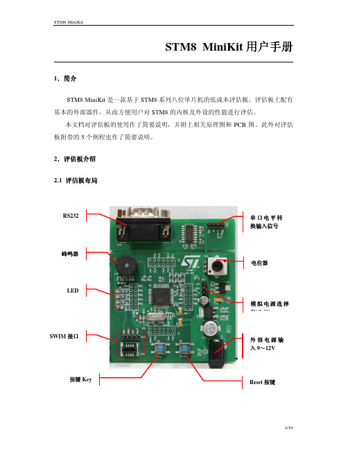
2．评估板介绍 2.1 评估板评估板布局布局2.2 原理图原理图与与PCB 原理图：PCB：3．参考代码说明随盘附赠的CD中共包含5个例程：Music：音乐播放例程；CSS：时钟切换及时钟安全系统的使用例程；Sinwave：正弦波发生例程；LED：LED控制例程；UART：串口与PC通讯例程；注：1)本例程仅适用于STM8S MiniKit评估板。

且调试时请确认模拟电源选择跳线已经连接到5V/3.3V。

2)所有的例程均使用Cosmic C语言编译器，用户请预先安装Cosmic C编译器。

3)所有项目均基于STVD 4.1.0集成开发环境，用户请预先安装相应软件。

4)所有例程使用STLink作为在线调试工具，请在进行在线调试前确认PC与STLink的硬件连接。

3.1 Music例程说明项目描述本例程通过采用pwm信号驱动蜂鸣器播放音乐并调节音量与音调，来说明如何使用Timer,ADC,GPIO,TLI:使用HSI为系统时钟源，并配置恰当的分频比；Timer2 CC1通道配置为PWM模式用以驱动蜂鸣器；Timer4 溢出中断用作LED1,LED2,LED3闪烁的时基；TLI（PD7)中断用来切换音乐的音调；ADC 采样电位器电压来调节占空比以控制音量。

项目文件main.c 包含"main" 函数的主程序stm8_interrupt_vector.c 中断向量表硬件环境将在线调试工具与目标板通过swim接口相连；在J1接口连接9~12v的直流电；使用电位器来调节蜂鸣器音量；使用按键可在高音调和低音调之间切换；如何开始可按照如下步骤调试：1)直接打开已经建立好的项目(..\Demo\Music\Demo.stw)，或创建一个项目并且配置好所有的项目选项（可按默认值配置）；2)编译这个项目Project->Rebuild all；3)下载程序到MCU进行调试：Debug->Start/Stop Debug Session4)运行程序：Debug->Run (F5)调节评估板上的电位器RV1来调节BUZZ音量；用按键来切换乐曲的音调；3个LED灯(LD1, LD2, LD3) 依次点亮。

Features included in iSolution LiteInclude:Live Measurement and Overlay SettingsUsers can perform measurements on the live preview image, using the crosshair or grid masks to center and count. The grid masks include calibration data. Calibration marker (scale bar) can be placed on the live preview image. The marker (scale bar) can also be burned on each captured image automatically. Any standard file format image can be chosen to see it above live preview image.Calibration (Auto, Manual)All measurements start with an accurate calibration. Auto, Semi-Auto calibration functions allow the software to calculate the pixels-per-unit value automatically. Only setting the unit for the calibration scale and the distance between the scale marks is needed. This feature greatly improves the accuracy and repetition of measurements. Manual calibrations are easily added and saved for recall from a drop down menu. All calibrations can be saved as files, which let the calibration be retrieved by simply opening the saved files later.Calibration can be protected by password option. Two password options, one in calibration menu itself and the other in camera resolution option, protect calibration by unexpected change. A scale bar can be permanently added to each image. Scale bar properties for color, size and text are simple to optimize for any image background.Z-Axis Extended Focus Imaging (EFI), with displacement compensation for stereo microscopesSamples with curves or of varying heights are difficult to bring into focus under highly magnified conditions. And more a stereomicroscope takes images with tilting due to its own structural characteristics. Thus, each image is out of its supposed position when you move microscope to the Z-axis getting the right focus. Our displacement compensation function allows you to rearrange these images automatically and manually.Software can combine a stack of images sequentially captured at different levels of focus and combine them into a single in-focus image. You can count on our software not to leave any trace of the composites.3D Visualization. . . clearly view complex structuresA Three-dimensional picture can be created from any image. The 3-D presentation is based upon intensity values of the image and can be displayed as a normal or wire frame image. Z axis information can easily be adjusted to optimize the 3-D effect. To better visualize an image in 3-D, software offers full 360 degrees of rotation on X-Y-Z axis. A 3D image can then saved in JPG, TIF or BMP format.Image Stitching. . . create a mosaic of the “Big Picture”With our software, you can create auto and manual composites of continuously captured images in order to minimize the reduction in the field-of-view that typically comes with increased magnification. Combined images are automatically corrected for brightness without leaving any stitching mark. Live Image Comparison. . . for fast inspection and size verificationFor QA testing or quick go/no-go inspections any stored image can be used as a reference image onto which the live preview image is projected.Time Lapse Capture and Movie File Production. . . Import into Power PointSoftware features a Time Lapse Capture function that supports TIF, BMP and JPG file formats. The Time Lapse Capture function also includes an Auto Save feature byyyyy/mm/dd/hour/minute/second. You can save video movie recordings in AVI, MPG, MPEG, and MOV formats.Combine Image Planes - Fluorescence ImagingMerge and pseudo color monochrome images into a single RGB composite.Export Into Excel® - with one mouse clickA single mouse click exports the original image with measurement, calibration, annotation overlay,measurement data, statistics, and chart.Manual Measurement Tools - Including Various Perpendicular DistanceSoftware’s versatile manual measurement features include tools for measuring lengths, areas, and angles and can even auto detect an object's outline and then make specified measurements. The software is equipped with a wide choice of powerful measurement tools including 3-point circle functionality, Npoint circle measurement functionality, parallel line distance measurement, perpendicular distance measurement and object distance measurement. In addition, a zoom-in window can be used to determine the accurate measuring point of an object.Once you've measured a specimen you can easily export all of the images, measurement data and statistics to an Excel® file. With iSolution Lite, comprehensive statistics and data are just one effortless mouse click away.Line ProfilingSingle, multiple, parallel and polyline commands provide Gray/Red/Green/Blue intensity values for specific lines within an image. The profile data of each pixel on the line can be exported to MS Excel. Auto TraceUsing an automatic edge detection algorithm, our software will perform an auto trace measurement function around a closed object. This function greatly increases accuracy and saves time when making measurements of complex shapes.Image ProcessingManual Brightness, Contrast, Gamma, Background Subtraction, Shading Correction, Histogram, Clone, Crop, AOI, Resize, Rotate, Split, Merge Monochrome series into RGB Color, Combine different exposure Images for highlight reduction, Image Mode Change, Grayscale, RGB, HSB, YUV Pseudo Color view, Full range of enhancement and morphology filters 8bit and 16bit per channel Manual MeasurementsPoint Count, Straight Line, Circle by radius, Circle by N points, Circle by diameter, Circle by 3 points, rectangle, polygon, polyline, splice lines from a common point, auto trace, angle parallel lines, perpendicular width, perpendicular from common line, angle between 2 lines, distance, perpendicular distance.Shading CorrectionThe edge parts of captured image by low magnification have background shading frequently, which can be removed by the shading correction function. The color of the original image remains the same though. A standard image is acquired from a blank space on the slide glass, or from an out of focus image in a metallurgical specimen. Such a standard image is used to correct the background shading of all other captured images.AnnotationLine, arrow, polyline, spline, rectangle, ellipse, textRegion of Interest- ROI. . . . with unique add/subtract capabilityRectangle, arbitrary rectangle, circle, arbitrary ellipse, polyline, spline, magic wand ROI itself can be saved to work with other images. The saved ROI can be placed on the exact same location of other images.View and Zoom ImageManual zoom In-Out, User Defined, Fit to Window, 1600% Zoom in Window for Accurate Edge Detect, sizeable context Window to view all open ImagesImage EditingUndo, Redo, Copy, Paste, Paste New, Delete, Delete All, Annotate, Image InformationSave OptionsTXT File Format, image and measurement data together in Proprietary .img File Format for future editing and data collectionSupported Image File Formatsjpg, jpeg, tif, tiff, bmp, gif, pcx, tga, mpg, mpeg, avi, mov, img, rpt, txt and etc.Report GeneratorCreate Report, Insert Image and Data, Insert other OLE ObjectsWindow ViewSplit Horizontal, Split Vertical, Cascade, Tile Horizontal, Tile Vertical, Arrange icons, Dynamic User Interface (UI), Classic, ModernTime Lapse Sequence ControlPlay Forward, Backward, Making Movie File (mpg, avi, mov) with Still Images, Split Single Image from Sequence FilePerfect Focus EnhancementiSolution FL implements a perfect function of focus compensation irrespective of the status of lights and specimen.Reflected Light SubtractioniSolution FL creates clear, evenly illuminated images by removing the bright saturated light from a highly reflective sample.System Requirements• PC with a Pentium-class processor; Pentium 300MMX or higher recommended• Microsoft Windows Win7/Vista/WinXP/2000/ME/Win98SE operating system• 32 MB of RAM or more (128 MB recommended)• 15 MB or more hard-disk space (50 MB recommended)• CD-ROM drive• VGA or higher-resolution monitor; Super VGA recommended (1024 x 768 pixel and 24 bit and more color support video card is recommended)• Microsoft Mouse or compatible pointing device• USB- or LPT-port for hardware key (depends on delivery).Supported imaging devices1. TWAIN Driver2. DirectShow/ WDM (Windows driver mode) driver3. i-Link DevicesAll PixeLINK cameras.Optronics digital cameras- MicroFire- MacroFire- QuantiFire and QuantiFire XI- Microcast- All MPX series cameras- All QPX series camerasJenoptik ProgRes digital cameras- C3 (cooled and non-cooled)- C5 (cooled and non-cooled)- C14- ProgRes CF and CFScan (cooled, non-cooled, and scan)- ProgRes MF (cooled, non-cooled, and scan)-ProgRes all CMOS cameras.Nikon digital cameras- DS-U2 Fi1- DS 5M/2M-U2- DS 5M/2M-U1- DXM 1200C- DXF 1200FPixera digital camera- Penguin series all models- Pro series all modelsScion corporation digital camera-CFW series all modelsMatrix vision-mvBlueFox digital cameraArtray- ARTCAM-500MI- ARTCAM-300MI- ARTCAM-200MI- ARTCAM-130MI (color, mono, and NIR) - ARTCAM-036MI (color, mono, and TWIN) - ARTCAM-500P- ARTCAM-200SH- ARTCAM-150P-II (color and mono)- ARTCAM-098 (color and mono)- ARTCAM-34MCLumenera- Infinity 1 series all models- Infinity 2 series all models- Infinity 3 series all models- Infinity X and Infinity X-21XLi camera- M series cameras- DC series cameras- DX series camerasSpot digital camera- Insight- FlexQimaging digital cameras- MicroPublisher- RetigaAll Leica digital cameras by TWAINCarl Zeiss AxioCam by TWAINFlashBus frame grabber- Spectrim Lite- Spectrim Pro- MV LiteMatrox frame grabber- Meteor IIAvermedia frame grabber- EZMakerConsumer digital camerasIMT i-Solution Inc. 。

FCC StatementThis equipment has been tested and found to comply with the limits for a Class B digital device, pursuant to part15of the FCC rules.These limits are designed to provide reasonable protection against harmful interference in a residential installation.This equipment generates,uses and can radiate radio frequency energy and,if not installed and used in accordance with the instructions, may cause harmful interference to radio communications.However,there is no guarantee that interference will not occur in a particular installation.If this equipment does cause harmful interference to radio or television reception,which can be determined by turning the equipment off and on,the user is encouraged to try to correct the interference by one or more of the following measures:-Reorient or relocate the receiving antenna.-Increase the separation between the equipment and receiver.-Connect the equipment into an outlet on a circuit different from that to which the receiver is connected.-Consult the dealer or an experienced radio/TV technician for help.To assure continued compliance,any changes or modifications not expressly approved by the party.Responsible for compliance could void the user’s authority to operate this equipment.This equipment complies with Part15of the FCC Rules.Operation is subject to the following two conditions:(1)This device may not cause harmful interference,and(2)This device must accept any interference received,including interference that may cause undesired operation.FCC Radiation Exposure Statement:The equipment complies with FCC Radiation exposure limits set forth for uncontrolled enviroment. This equipment should be installed and operated with minimum distance20cm between the radiator and your body.。

GAMIT/GLOBK软件使用手册一软解介绍GAMIT软件最初由美国麻省理工学院研制，后与美国SCRIPPS海洋研究所共同开发改进。

该软件是世界上最优秀的GSP定位和定轨软件之一，采用精密星历和高精度起算点时，其解算长基线的相对精度能达到10—9量级, 解算短基线的精度能优于1mm，特点是运算速度快、版木更新周期短以及在精度许可范围内自动化处理程度高等, 因此应用相当广泛.GAMIT软件由许多不同功能的模块组成, 这些模块可以独立地运行.按其功能可分成两个部分: 数据准备和数据处理。

此外, 该软件还带有功能强大的shell程序。

目前，比较著名的GPS数据处理软件主要有美国麻省理工学院（MIT）和海洋研究所(SIO)联合研制的GAMIT/GLOBK软件、瑞士伯尔尼大学研制的BERNESE软件、美国喷气推进实验室（JPL）研制的GIPSY软件等。

GAMIT/GLOBK和BERNESE软件采用相位双差数据作为基本解算数据，GIPSY软件采用非差相位数据作为基本解算数据，在精度方面，三个软件没有明显的差异，都可得到厘米级的点位坐标精度。

相比较而言，GIPSY软件为美国军方研制的软件，国内只能得到它的执行程序，在国内，它的用户并不多，BERNESE软件需要购买，它的用户稍微多一点，GAMIT/GLOBK软件接近于自由软件，在国内拥有大量用户。

GLOBK软件核心思想是卡尔曼滤波（卡尔曼滤波理论是一种对动态系统进行数据处理的有效方法，它利用观测向量来估计随时间不断变化的状态向量），其主要目的是综合处理多元测量数据。

GLOBK的主要输人是经GAMIT处理后的h-file和近似坐标, 当然，它亦己成功地应用于综合处理其它的GPS软件（如Bernese和GIPSY)产生的数据以及其它大地测量和SLR 观测数据。

GLOBK的主要输出有测站坐标的时间序列、测站平均坐标、测站速度和多时段轨道参数，GLOBK可以有效地检验不同约束条件下的影响，因为单时段分析使用了非常宽松的约束条件，所以在GLOBK中就可以对任一参数强化约束.GAMIT/GLOBK和BERNESE采用双差作为数据分析的基本观测量,它们的缺陷是不能直接解算钟差参数，只能给出测站的基线结果，除测站坐标参数之外，这些软件还可以解算的参数有：卫星轨道参数、卫星天线偏差、光压参数、地球自转参数、地球质量中心变化、测站对流层延迟参数、电离层改正参数等，这使这些软件的应用从大地测量学已逐渐延伸到地球动力学、卫星动力学、气象学以及地球物理学等领域，并取得了很多成果.GAMIT软件的运行平台是UNIX操作系统,目前，它可在Sun、HP、IBM/RISC、DEC、LINUX等基于intel处理器的工作站上运行。

Package‘genogeographer’October13,2022Type PackageTitle Methods for Analysing Forensic Ancestry Informative MarkersVersion0.1.19Author Torben TvedebrinkMaintainer Torben Tvedebrink<**************.dk>Depends R(>=3.1.0)Imports leaflet,shiny,shinyjs,knitr,DT,shinycssloaders,purrr,dplyr,magrittr,tidyr,ggplot2,tibble,forcats,readr,rmarkdown,rio,maps,shinyWidgets,rlangSuggests tidyverseDescription Evaluates likelihood ratio tests for alleged ancestry.Implements the methods of Tvede-brink et al(2018)<doi:10.1016/j.tpb.2017.12.004>.License GPL(>=2)Encoding UTF-8LazyData trueRoxygenNote6.1.1NeedsCompilation noRepository CRANDate/Publication2019-09-2710:20:08UTCR topics documented:app_genogeo (2)bar_colour (2)error_bar_plot (3)exponent_tilt (3)genogeo (4)genogeographer (5)kidd_loci (5)LR_table (6)main_alleles (7)12bar_colour map_plot (7)pops_to_DB (8)profile_AA_x0 (9)profile_admixture (9)random_AIMs_profile (10)seldin_loci (10)simulate_pops (11)Index12 app_genogeo Shiny application for GenoGeoGrapherDescriptionShiny application for GenoGeoGrapherUsageapp_genogeo(db_list=NULL,reporting_panel=TRUE)Argumentsdb_list A named list of databases of reference populations.Each component is expected to be returned from pops_to_DB.reporting_panelLogical.Should report generate and download be available after sample analy-sis.bar_colour bar_colourDescriptionCreates the colour scale for the accepted and rejected populations based on z-score and the log likelihood(log P).Usagebar_colour(df,alpha=1)Argumentsdf A data.frame with at least three coloums.Thefirst column is the logP,the second logical(z_score accept/reject),the third a unique naming column.alpha Should the alpha opacity be applied?And what value,1=solid,0=transparent.error_bar_plot3 error_bar_plot Plot log likelihoods of profiles with approximate confidence intervalsDescriptionPlots the estimated profile probabilities in each population.The colour depends on the profiles likelihood and rejection/acceptance(blue/red)based on z-scoreUsageerror_bar_plot(data)Argumentsdata The output from the genogeo functionValueA barplot of the log likelihoods for each population with confidence limitsAuthor(s)Torben Tvedebrink,<**************.dk>Examplesdf_<-simulate_pops(pop_n=20,aims_n=50)df_db<-pops_to_DB(df_)profile<-random_AIMs_profile(df_db,keep_pop=TRUE)profile$pop[1]#The true populationresult<-genogeo(profile[,c("locus","x0")],df=df_db)error_bar_plot(result)exponent_tilt P-values from Importing Sampling using Exponential tiltingDescriptionP-values from Importing Sampling using Exponential tiltingUsageexponent_tilt(x0,x1,n,p_limit=0.1,B=500,return_all=FALSE)4genogeoArgumentsx0Allele count of profilex1Population allele countn Sampled alleles in total in populationp_limit Upper limit to which we use the normal approximationB An integer specifying the number of importance samples.return_all Default is FALSE.If TRUE:Returns p-value,standard deviation,and method (and diagnostics).DetailsThe method of importance sampling described in Tvedebrink et al(2018),Section2.3is imple-mented.It relies on exponential tilting of the proposal distribution using in the importance sam-pling.ValueIf return_all=FALSE the p-value is returned.Otherwise list of elements(see return_all)is returned.genogeo Likelihood ratio tests for AIMsDescriptionComputes the likelihood ratio test statistics for each population in a database of reference popula-tions.Usagegenogeo(profile,df,CI=0.95,min_n=75,grouping="pop",tilt=FALSE,...)Argumentsprofile The AIMs profile encoded as returned by the profile_AA_x0function.df The database of reference populations as returned by the pops_to_DB function.CI The confidence level used to reject or accept the various hypotheses(between0 and1).min_n Minimum number of individuals in each database samplegrouping should"pop"(the default)or"meta"be used for aggregating the results.Can also be"cluster"if this variable is defined in the input database.tilt Should exponential titling be used to obtain more accurate$p$-values in the distribution’s tail(currently not implemented)...Further arguments that are passed to other functionsgenogeographer5ValueA tibble containing the$z$-scores,$p$-values etc for each population.Examplesdf_<-simulate_pops(pop_n=20,aims_n=50)df_db<-pops_to_DB(df_)profile<-random_AIMs_profile(df_db,keep_pop=TRUE)profile$pop[1]#The true populationresult<-genogeo(profile[,c("locus","x0")],df=df_db)genogeographer genogeographer:Methods for analysing forensic Ancestry Informa-tive MarkersDescriptionThe genogeographer package provides:genogeo()genogeo functionsSee?genogeokidd_loci Kenn Kidd Lab markersDescriptionList of markers identified by Kenn Kidd lab.Usagekidd_lociFormatList of55markerslocus Locus/Marker namesSourceK.K.Kidd et al.Progress toward an efficient panel of SNPs for ancestry inference.Forensic Science International:Genetics10(2014)23–326LR_table LR_table Compute pairwise likelihood ratiosDescriptionFor each pair of a specified vector of profiles the likelihood ratios are computed.The list can include all populations in the data or only a subset.We may for inferral purposes restrict to ratios including at least one"accepted"population.UsageLR_table(result_df,lr_populations=NULL,only_accepted=TRUE,CI=0.95,digits=NULL,keep_logP=FALSE)Argumentsresult_df The output from genogeolr_populations A vector of population names(pop in result_df).If NULL all populations are used.only_accepted Restrict the ratios to include minimum one accepted population.CI The level of confidence interval to be computeddigits If rounding of the output should be performed.keep_logP Logical.Should the logP’s be returned in outputValueA tibble with numerator and denominator populations with their log10LR and uncertainty.Author(s)Torben Tvedebrink<**************.dk>Examplesdf_<-simulate_pops(pop_n=4,aims_n=50)df_db<-pops_to_DB(df_)profile<-random_AIMs_profile(df_db,keep_pop=TRUE)profile$pop[1]#The true populationresult<-genogeo(profile[,c("locus","x0")],df=df_db)LR_table(result)main_alleles7 main_alleles AIMs markers in Precision ID Ancestry Panel(Thermo Fisher Scien-tific)DescriptionList of markers with their main and alternative allele.The markers is the union of Seldin’s and Kidd’s markers.Usagemain_allelesFormatList of164markerslocus Locus/Marker namesmain_allele The main allele(alleles are in lexicographic order)other_allele The other variantmap_plot Plot LTR z-scores on mapDescriptionPlots the results from LRT on a map based on lat/lon info in the database.If no location is found in the data(ing simulte_pops)nothing is plotted.Usagemap_plot(data)Argumentsdata The output from the genogeo functionValueA map with population z-scores at their geographic originAuthor(s)Torben Tvedebrink,<**************.dk>8pops_to_DB Examplesdf_<-simulate_pops(pop_n=4,aims_n=50)df_db<-pops_to_DB(df_)profile<-random_AIMs_profile(df_db,keep_pop=TRUE)profile$pop[1]#The true populationresult<-genogeo(profile[,c("locus","x0")],df=df_db,min_n=0)result$lon<-runif(n=4,min=-125,max=125)result$lat<-runif(n=4,min=-50,max=80)##Not run:map_plot(result)pops_to_DB Pre-compute the scores for a given reference databaseDescriptionConvert the counts from each population over a range of AIMs SNPs q to observed likelihood ratio test,its mean and variance.Based on these pre-computed the evaluation of a specific profile is done using genogeo with the resulting dataframe as df.Usagepops_to_DB(db,...)Argumentsdb A dataframe with columns similar to those of simulate_pops().If db contains information(recommended!)about"meta"(meta population)and"lat"/"lon"(location)these are carried over into the calculations...Additional arguments passed to score_add_dfValueA tibble with population and locus specific score informationExamplesdf_<-simulate_pops(pop_n=4,aims_n=50)df_db<-pops_to_DB(df_)profile_AA_x09 profile_AA_x0Function that compute the genotype probability for each population(rows in df)DescriptionFunction that compute the genotype probability for each population(rows in df)Usageprofile_AA_x0(AA_profile,df,select=c("locus","x0"),keep_dropped=FALSE)ArgumentsAA_profile A tibble/data.frame with columns’locus’,’A1’and’A2’holding the separated version of a genotype,eg.AG->A1:A,A2:Gdf The database with main alleles per locusselect Which columns to returnkeep_dropped Logical.Keep the non-matching alleles(compared to‘db‘)and those with geno-type‘NN‘profile_admixture Compute the z-score(and more)for admixed hypothesesDescriptionCompute the z-score(and more)for admixed hypothesesUsageprofile_admixture(x0,df,hyp=NULL,grouping="meta",return_all=FALSE,calc_logP=TRUE,...)Argumentsx0A data frame/tibble with two columns:‘locus‘and‘x0‘df A tibble of reference profiles(as for‘genogeo‘)hyp If NULL all levels of‘grouping‘is crossed and looped over as pairwise hy-potheses.If a single level of‘grouping‘,this value is crossed with the remaininglevels.If vector of two levels this is the only tested hypothesis.grouping Should the calculations be for meta populations("meta")or sample populations ("pop")?return_all Should z-score be returned(FALSE)or all locus results(TRUE)?calc_logP Should log P(Geno|Hyp)be calculated(TRUE)or not(FALSE)?...additional arguments passed on to other functions10seldin_lociValueA tibble of z-scores,or a list of pairwise results if‘return_all=TRUE‘random_AIMs_profile Simulate a random AIMs profileDescriptionUse the information from pops_to_DB to simulate a profile from a random or given population.The sampling is done with respect to the null hypothesis,such that the total count is adjusted accordingly.For further details see Tvedebrink et al(2018),Section3.1(Simulations).Usagerandom_AIMs_profile(df,grouping="pop",population=NULL,n=FALSE,keep_pop=FALSE)Argumentsdf Database of reference profiles as returned by pops_to_DBgrouping Simualte from pop(default)or meta.population The population to sample from.If NULL chosen at random.n Use numbers of samples as weights to choose the population randomlykeep_pop Keep information on populationAuthor(s)Torben Tvedebrink<**************.dk>seldin_loci Seldin Lab markersDescriptionList of markers identified by Seldin lab.Usageseldin_lociFormatList of122markerslocus Locus/Marker namessimulate_pops11SourceKosoy et al.Ancestry Informative Marker Sets for Determining Continental Origin and Admixture Proportions in Common Populations in America.HUMAN MUTATION,V ol.30,No.1,69–78, 2009.simulate_pops Simulate random populationsDescriptionSimulate random populationsUsagesimulate_pops(pop_n=100,pop_names=NULL,pop_totals=NULL,aims_n=50,aims_names=NULL)Argumentspop_n Number of populations to simulatepop_names Their names.If NULL:The names are"pop_001"through"pop_pop_n"pop_totals How many observations/sampled individuals per population.If one number this is used as parameter in a Poisson distributionaims_n Number of AIMsaims_names Their names.If NULL:The names are"rs_001"through"rs_aims_n"Author(s)Torben Tvedebrink<**************.dk>Index∗datasetskidd_loci,5main_alleles,7seldin_loci,10app_genogeo,2bar_colour,2error_bar_plot,3exponent_tilt,3genogeo,4genogeographer,5genogeographer-package(genogeographer),5kidd_loci,5LR_table,6main_alleles,7map_plot,7pops_to_DB,8profile_AA_x0,9profile_admixture,9random_AIMs_profile,10seldin_loci,10simulate_pops,1112。

Package‘geohashTools’October21,2023Version0.3.3Title Tools for Working with GeohashesMaintainer Michael Chirico<*************************>Depends R(>=3.0.0)Description Tools for working with Gustavo Niemeyer's geohash coordinate system,includ-ing API for interacting with other common R GIS libraries.URL https:///MichaelChirico/geohashToolsLicense MPL-2.0|file LICENSEImports methodsSuggests sf,sp,testthat(>=3.0.0),knitr,rmarkdown,ggplot2Config/testthat/edition3VignetteBuilder knitrEncoding UTF-8RoxygenNote7.2.3NeedsCompilation yesAuthor Michael Chirico[aut,cre],Dmitry Shkolnik[ctb]Repository CRANDate/Publication2023-10-2120:10:02UTCR topics documented:gh_decode (2)gh_encode (3)gh_neighbors (4)gis_tools (5)utils (6)Index812gh_decodegh_decode Geohash decodingDescriptionConvert geohash-encoded strings into latitude/longitude coordinatesUsagegh_decode(geohashes,include_delta=FALSE,coord_loc= c )Argumentsgeohashes character or factor vector or of input geohashes.There’s no need for allinputs to be of the same precision.include_delta logical;should the cell half-width delta be included in the output?coord_loc character specifying where in the cell points should be mapped to;cell cen-troid is mapped by default;case-insensitive.See Details.Detailscoord_loc can be the cell’s center( c or centroid ),or it can be any of the8corners(e.g.s / south for the midpoint of the southern boundary of the cell,or ne / northeast for the upper-right corner.For factor input,decoding will be done on the levels for efficiency.Valuelist with the following entries:latitude numeric vector of latitudes(y-coordinates)corresponding to the input geohashes, with within-cell position dictated by coord_loclongitude numeric vector of longitudes(x-coordinates)corresponding to the input geohashes, with within-cell position dictated by coord_locdelta_latitude numeric vector of cell half-widths in the y direction(only included if include_delta is TRUEdelta_longitudenumeric vector of cell half-widths in the x direction(only included if include_deltais TRUEAuthor(s)Michael ChiricoReferences/(Gustavo Niemeyer’s original geohash service)gh_encode3Examples#Riddle me thisgh_decode( stq4s8c )#Cell half-widths might be convenient to include for downstream analysisgh_decode( tjmd79 ,include_delta=TRUE)gh_encode Geohash encodingDescriptionConvert latitude/longitude coordinates into geohash-encoded stringsUsagegh_encode(latitude,longitude,precision=6L)Argumentslatitude numeric vector of input latitude(y)coordinates.Must be in[-90,90).longitude numeric vector of input longitude(x)coordinates.Should be in[-180,180).precision Positive integer scalar controlling the’zoom level’–how many characters should be used in the output.Detailsprecision is limited to at most28.This level of precision encodes locations on the globe at a nanometer scale and is already more than enough for basically all applications.Longitudes outside[-180,180)will be wrapped appropriately to the standard longitude grid. Valuecharacter vector of geohashes corresponding to the input.NA in gives NA out.Author(s)Michael ChiricoReferences/(Gustavo Niemeyer’s original geohash service)4gh_neighborsExamples#scalar input is treated as a vectorgh_encode(2.345,6.789)#geohashes are left-closed,right-open,so boundary coordinates are#associated to the east and/or northgh_encode(0,0)gh_neighbors Geohash neighborhoodsDescriptionReturn the geohashes adjacent to input geohashesUsagegh_neighbors(geohashes,self=TRUE)gh_neighbours(geohashes,self=TRUE)Argumentsgeohashes character vector of input geohashes.There’s no need for all inputs to be of the same precision.self Should the input also be returned as a list element?Convenient for one-line usage/pipingDetailsNorth/south-pole adjacent geohashes are missing three of their neighbors;these will be returned as NA_character_.Valuelist with character vector entries in the direction relative to the input geohashes indicated by their name(e.g.value$south gives all of the southern neighbors of the input geohashes).The order is self(if self=TRUE),southwest,south,southeast,west,east,northwest,north, northeast(reflecting an easterly,then northerly traversal of the neighborhod).Author(s)Michael ChiricoReferences/(Gustavo Niemeyer’s original geohash service)gis_tools5Examplesgh_neighbors( d7q8u4 )gis_tools Helpers for interfacing geohashes with sp/sf objectsDescriptionThese functions smooth the gateway between working with geohashes and geospatial information built for the major geospatial packages in R,sp and sf.Usagegh_to_sp(geohashes)gh_to_spdf(...)gh_to_sf(...)gh_covering(SP,precision=6L,minimal=FALSE)##Default S3method:gh_to_spdf(geohashes,...)##S3method for class data.framegh_to_spdf(gh_df,gh_col= gh ,...)Argumentsgeohashes character vector of geohashes to be converted to polygons....Arguments for subsequent methods.SP A Spatial object(requires bbox and proj4string methods,and over if minimal is TRUE)precision integer specifying the precision of geohashes to use,same as gh_encodeminimal logical;if FALSE,the output will have all geohashes in the bounding box ofSP;if TRUE,any geohashes not intersecting SP will be removed.gh_df data.frame which1)contains a column of geohashes to be converted to poly-gons and2)will serve as the data slot of the resultant SpatialPolygonsDataFrameobject.gh_col character column name saying where the geohashes are stored in gh_df. Detailsgh_to_sp relies on the gh_decode function.Note in particular that this function accepts any length of geohash(geohash-6,geohash-4,etc.)and is agnostic to potential overlap,though duplicates will be caught and excluded.gh_to_spdf.data.frame will use match.ID=FALSE in the call to SpatialPolygonsDataFrame.Pleasefile an issue if you’d like this to be moreflexible.gh_to_sf is just a wrapper of st_as_sf around gh_to_spdf;as such it requires both sp and sf packages to work.ValueFor gh_to_sp,a SpatialPolygons object.For gh_to_spdf,a SpatialPolygonsDataFrame object.For gh_to_sf,a sf object.Examples#get the neighborhood of this geohash in downtown Apia as an sp objectdowntown= 2jtc5xapia_nbhd=unlist(gh_neighbors(downtown))apia_sp=gh_to_sp(apia_nbhd)#all geohashes covering a random sampling within Apia:apia_covering=gh_covering(smp<-sp::spsample(apia_sp,10L, random ))apia_sf=gh_to_sf(apia_nbhd)utils Geohash utilitiesDescriptionVarious common functions that arise when working often with geohashesUsagegh_delta(precision)Argumentsprecision integer precision level desired.ValueLength-2numeric vector;thefirst element is the latitude(y-coordinate)half-width at the input precision,the second element is the longitude(x-coordinate).NoteCaveat coder:not much is done in the way of consistency checking since this is a convenience function.So e.g.real-valued"precision"s will give results.Author(s)Michael ChiricoReferences/(Gustavo Niemeyer’s original geohash service)Examplesgh_delta(6)Indexgh_covering(gis_tools),5gh_decode,2,5gh_delta(utils),6gh_encode,3,5gh_neighbors,4gh_neighbours(gh_neighbors),4gh_to_sf(gis_tools),5gh_to_sp(gis_tools),5gh_to_spdf(gis_tools),5gis_tools,5sf,5,6sp,5Spatial,5SpatialPolygons,6 SpatialPolygonsDataFrame,5,6st_as_sf,6utils,68。

Package‘geojsonR’January12,2023Type PackageTitle A GeoJson Processing ToolkitVersion1.1.1Date2023-01-12BugReports https:///mlampros/geojsonR/issuesURL https:///mlampros/geojsonRDescription Includes functions for processing GeoJson ob-jects<https:///wiki/GeoJSON>rely-ing on'RFC7946'<https:///doc/pdf/rfc7946.pdf>.The geoj-son encoding is based on'json11',a tiny JSON li-brary for'C++11'<https:///dropbox/json11>.Further-more,the source code is exported in R through the'Rcpp'and'RcppArmadillo'packages. License MIT+file LICENSEEncoding UTF-8Copyright inst/COPYRIGHTSSystemRequirements libarmadillo:apt-get install-y libarmadillo-dev(deb)Depends R(>=3.2.3)Imports Rcpp(>=0.12.9),R6LinkingTo Rcpp,RcppArmadillo(>=0.7.6)Suggests testthat,covr,knitr,rmarkdownVignetteBuilder knitrRoxygenNote7.2.3NeedsCompilation yesAuthor Lampros Mouselimis[aut,cre](<https:///0000-0002-8024-1546>), Dropbox Inc[cph]Maintainer Lampros Mouselimis<***************************>Repository CRANDate/Publication2023-01-1209:20:06UTC12Dump_From_GeoJson R topics documented:Dump_From_GeoJson (2)Features_2Collection (3)FROM_GeoJson (4)FROM_GeoJson_Schema (5)merge_files (7)save_R_list_Features_2_FeatureCollection (8)shiny_from_JSON (10)TO_GeoJson (10)Index18 Dump_From_GeoJson returns a json-dump from a geojsonfileDescriptionreturns a json-dump from a geojsonfileUsageDump_From_GeoJson(url_file)Argumentsurl_file either a string specifying the input path to afile OR a valid url(beginning with ’http..’)pointing to a geojson objectValuea character string(json dump)Examples##Not run:library(geojsonR)res=Dump_From_GeoJson("/myfolder/point.geojson")##End(Not run)Features_2Collection3Features_2Collection creates a FeatureCollection dump from multiple Feature geojson ob-jectsDescriptioncreates a FeatureCollection dump from multiple Feature geojson objectsUsageFeatures_2Collection(Features_files_vec,bbox_vec=NULL,write_path=NULL,verbose=FALSE)ArgumentsFeatures_files_veca character vector specifying paths tofiles(Feature geojson objects)bbox_vec either NULL or a numeric vectorwrite_path either NULL or a character string specifying a valid path to afile(preferably with a.geojson extension)where the output data will be saved verbose a boolean.If TRUE then information will be printed out in the console DetailsThe Features_2Collection function utilizes internally a for-loop.In case of an error set the verbose parameter to TRUE tofind out whichfile leads to this error.Valuea FeatureCollection dumpExamples##Not run:library(geojsonR)vec_files=c("/myfolder/Feature1.geojson","/myfolder/Feature2.geojson","/myfolder/Feature3.geojson","/myfolder/Feature4.geojson","/myfolder/Feature5.geojson")res=Features_2Collection(vec_files,bbox_vec=NULL)4FROM_GeoJson ##End(Not run)FROM_GeoJson reads GeoJson dataDescriptionreads GeoJson dataUsageFROM_GeoJson(url_file_string,Flatten_Coords=FALSE,Average_Coordinates=FALSE,To_List=FALSE)Argumentsurl_file_stringa string specifying the input path to afile OR a geojson object(in form of acharacter string)OR a valid url(beginning with’http..’)pointing to a geojsonobjectFlatten_Coords either TRUE or FALSE.If TRUE then the properties member of the geojsonfile will be omitted during parsing.Average_Coordinateseither TRUE or FALSE.If TRUE then additionally a geojson-dump and theaverage latitude and longitude of the geometry object will be returned.To_List either TRUE or FALSE.If TRUE then the coordinates of the geometry object will be returned in form of a list,otherwise in form of a numeric matrix.DetailsThe FROM_GeoJson function is based on the’RFC7946’specification.Thus,geojsonfiles/strings which include property-names other than the’RFC7946’specifies will return an error.To avoid errors of that kind a user should take advantage of the FROM_GeoJson_Schema function,which is not as strict concerning the property names.Valuea(nested)listExamples##Not run:library(geojsonR)#INPUT IS A FILEres=FROM_GeoJson(url_file_string="/myfolder/feature_collection.geojson")#INPUT IS A GEOJSON(character string)tmp_str= {"type":"MultiPolygon","coordinates":[[[[102.0,2.0],[103.0,2.0],[103.0,3.0],[102.0,3.0],[102.0,2.0]]], [[[100.0,0.0],[101.0,0.0],[101.0,1.0],[100.0,1.0],[100.0,0.0]],[[100.2,0.2],[100.8,0.2],[100.8,0.8],[100.2,0.8],[100.2,0.2]]]]}res=FROM_GeoJson(url_file_string=tmp_str)#INPUT IS A URLres=FROM_GeoJson(url_file_string="http://www.EXAMPLE_web_page.geojson") ##End(Not run)FROM_GeoJson_Schema reads GeoJson data using a one-word-schemaDescriptionreads GeoJson data using a one-word-schemaUsageFROM_GeoJson_Schema(url_file_string,geometry_name="",Average_Coordinates=FALSE,To_List=FALSE)Argumentsurl_file_stringa string specifying the input path to afile OR a geojson object(in form of acharacter string)OR a valid url(beginning with’http..’)pointing to a geojsonobjectgeometry_name a string specifying the geometry name in the geojson string/file.The geome-try_name functions as a one-word schema and can significantly speed up theparsing of the data.Average_Coordinateseither TRUE or FALSE.If TRUE then additionally a geojson-dump and theaverage latitude and longitude of the geometry object will be returned.To_List either TRUE or FALSE.If TRUE then the coordinates of the geometry object will be returned in form of a list,otherwise in form of a numeric matrix.DetailsThis function is appropriate when the property-names do not match exactly the’RFC7946’spec-ification(for instance if the geometry object-name appears as location as is the case sometimes in mongodb queries).The user can then specify the geometry_name as it exactly appears in the .geojson string/file(consult the example for more details).If no geometry_name is given then recur-sion will be used,which increases the processing time.In case that the input.geojson object is of type:Point,LineString,MultiPoint,Polygon,GeometryCollection,MultiLineString,MultiPolygon, Feature or FeatureCollection with a second attribute name:coordinates,then the geometry_name parameter is not necessary.Valuea(nested)listExampleslibrary(geojsonR)#INPUT IS A GEOJSON(character string)tmp_str= {"name":"example_name","location":{"type":"Point","coordinates":[-120.24,39.21]}}res=FROM_GeoJson_Schema(url_file_string=tmp_str,geometry_name="location")merge_files7 merge_files merge jsonfiles(or any kind of textfiles)from a directoryDescriptionmerge jsonfiles(or any kind of textfiles)from a directoryUsagemerge_files(INPUT_FOLDER,OUTPUT_FILE,CONCAT_DELIMITER="\n",verbose=FALSE)ArgumentsINPUT_FOLDER a character string specifying a path to the input folderOUTPUT_FILE a character string specifying a path to the outputfileCONCAT_DELIMITERa character string specifying the delimiter to use when merging thefilesverbose either TRUE or FALSE.If TRUE then information will be printed in the console. DetailsThis function is meant for jsonfiles but it can be applied to any kind of textfiles.It takes an input folder(INPUT_FOLDER)and an outputfile(OUTPUT_FILE)and merges allfiles from the IN-PUT_FOLDER to a single OUTPUT_FILE using the concatenation delimiter(CONCAT_DELIMITER).Examples##Not run:library(geojsonR)merge_files(INPUT_FOLDER="/my_folder/",OUTPUT_FILE="output_file.json")##End(Not run)save_R_list_Features_2_FeatureCollectioncreates a FeatureCollection from R list objects(see the details sectionabout the limitations of this function)Descriptioncreates a FeatureCollection from R list objects(see the details section about the limitations of this function)Usagesave_R_list_Features_2_FeatureCollection(input_list,path_to_file="",verbose=FALSE)Argumentsinput_list a list object that includes1or more geojson R list Featurespath_to_file either an empty string("")or a valid path to afile where the output FeatureCol-lection will be savedverbose a boolean.If TRUE then information will be printed out in the console Details•it allows the following attributes:’type’,’id’,’properties’and’geometry’•it allows only coordinates of type’Polygon’or’MultiPolygon’to be processed.In case of a’Polygon’there are2cases:(a.)Polygon WITHOUT interior rings(a numeric matrix is expected)and(b.)Polygon WITH interior rings(a list of numeric matrices is expected).See the test-cases if you receive an error for the correct format of the input data.In case of a ’MultiPolygon’both Polygons with OR without interior rings can be included.Multipolygons are of the form:list of lists where each SUBLIST can be either a numeric matrix(Polygon without interior rings)or a list(Polygon with interior rings)•the properties attribute must be a list that can take only character strings,numeric and integer values of SIZE1.In case that any of the input properties is of SIZE>1then it will throw an error.The input_list parameter can be EITHER created from scratch OR GeoJson Features(in form of a FeatureCollection)can be loaded in R and modified so that this list can be processed by this functionValuea FeatureCollection in form of a character stringa FeatureCollection saved in afileExamples##Not run:library(geojsonR)#------------------------------------------------#valid example that will save the data to a file#------------------------------------------------Feature1=list(type="Feature",id=1L,properties=list(prop1= id ,prop2=1.0234),geometry=list(type= Polygon ,coordinates=matrix(runif(20),nrow=10,ncol=2))) Feature2=list(type="Feature",id=2L,properties=list(prop1= non-id ,prop2=6.0987),geometry=list(type= MultiPolygon ,coordinates=list(matrix(runif(20),nrow=10,ncol=2),matrix(runif(20),nrow=10,ncol=2)))) list_features=list(Feature1,Feature2)path_feat_col=tempfile(fileext= .geojson )res=save_R_list_Features_2_FeatureCollection(input_list=list_features,path_to_file=path_feat_col,verbose=TRUE)#-------------------------------------#validate that the file can be loaded#-------------------------------------res_load=FROM_GeoJson_Schema(url_file_string=path_feat_col)str(res_load)#----------------------------------------------------#INVALID data types such as NA s will throw an ERROR#----------------------------------------------------Feature1=list(type="Feature",id=1L,properties=list(prop1=NA,prop2=1.0234),geometry=list(type= Polygon ,coordinates=matrix(runif(20),nrow=10,ncol=2))) list_features=list(Feature1,Feature2)10TO_GeoJsonpath_feat_col=tempfile(fileext= .geojson )res=save_R_list_Features_2_FeatureCollection(input_list=list_features,path_to_file=path_feat_col,verbose=TRUE)##End(Not run)shiny_from_JSON secondary function for shiny ApplicationsDescriptionsecondary function for shiny ApplicationsUsageshiny_from_JSON(input_file)Argumentsinput_file a character string specifying a path to afileDetailsThis function is meant for shiny Applications.To read a GeoJsonfile use either the FROM_GeoJson or FROM_GeoJson_Schema function.Valuea(nested)listTO_GeoJson converts data to a GeoJson objectDescriptionconverts data to a GeoJson objectconverts data to a GeoJson objectUsage#utl<-TO_GeoJson$new()Valuea ListMethodsTO_GeoJson$new()--------------Point(data,stringify=FALSE)--------------MultiPoint(data,stringify=FALSE)--------------LineString(data,stringify=FALSE)--------------MultiLineString(data,stringify=FALSE)--------------Polygon(data,stringify=FALSE)--------------MultiPolygon(data,stringify=FALSE)--------------GeometryCollection(data,stringify=FALSE) --------------Feature(data,stringify=FALSE)--------------FeatureCollection(data,stringify=FALSE)--------------MethodsPublic methods:•TO_GeoJson$new()•TO_GeoJson$Point()•TO_GeoJson$MultiPoint()•TO_GeoJson$LineString()•TO_GeoJson$MultiLineString()•TO_GeoJson$Polygon()•TO_GeoJson$MultiPolygon()•TO_GeoJson$GeometryCollection()•TO_GeoJson$Feature()•TO_GeoJson$FeatureCollection()•TO_GeoJson$clone()Method new():Usage:TO_GeoJson$new()Method Point():Usage:TO_GeoJson$Point(data,stringify=FALSE)Arguments:data a list specifying the geojson geometry objectstringify either TRUE or FALSE,specifying if the output should also include a geojson-dump(as a character string)Method MultiPoint():Usage:TO_GeoJson$MultiPoint(data,stringify=FALSE)Arguments:data a list specifying the geojson geometry objectstringify either TRUE or FALSE,specifying if the output should also include a geojson-dump(as a character string)Method LineString():Usage:TO_GeoJson$LineString(data,stringify=FALSE)Arguments:data a list specifying the geojson geometry objectstringify either TRUE or FALSE,specifying if the output should also include a geojson-dump(as a character string)Method MultiLineString():Usage:TO_GeoJson$MultiLineString(data,stringify=FALSE)Arguments:data a list specifying the geojson geometry objectstringify either TRUE or FALSE,specifying if the output should also include a geojson-dump(as a character string)Method Polygon():Usage:TO_GeoJson$Polygon(data,stringify=FALSE)Arguments:data a list specifying the geojson geometry objectstringify either TRUE or FALSE,specifying if the output should also include a geojson-dump(as a character string)Method MultiPolygon():Usage:TO_GeoJson$MultiPolygon(data,stringify=FALSE)Arguments:data a list specifying the geojson geometry objectstringify either TRUE or FALSE,specifying if the output should also include a geojson-dump(as a character string)Method GeometryCollection():Usage:TO_GeoJson$GeometryCollection(data,stringify=FALSE)Arguments:data a list specifying the geojson geometry objectstringify either TRUE or FALSE,specifying if the output should also include a geojson-dump(as a character string)Method Feature():Usage:TO_GeoJson$Feature(data,stringify=FALSE)Arguments:data a list specifying the geojson geometry objectstringify either TRUE or FALSE,specifying if the output should also include a geojson-dump(as a character string)Method FeatureCollection():Usage:TO_GeoJson$FeatureCollection(data,stringify=FALSE)Arguments:data a list specifying the geojson geometry objectstringify either TRUE or FALSE,specifying if the output should also include a geojson-dump(as a character string)Method clone():The objects of this class are cloneable with this method.Usage:TO_GeoJson$clone(deep=FALSE)Arguments:deep Whether to make a deep clone.Exampleslibrary(geojsonR)#initialize classinit=TO_GeoJson$new()#Examples covering all geometry-objects#Pointpoint_dat=c(100,1.01)point=init$Point(point_dat,stringify=TRUE)point#MultiPointmulti_point_dat=list(c(100,1.01),c(200,2.01))multi_point=init$MultiPoint(multi_point_dat,stringify=TRUE)multi_point#LineStringlinestring_dat=list(c(100,1.01),c(200,2.01))line_string=init$LineString(linestring_dat,stringify=TRUE)line_string#MultiLineStringmultilinestring_dat=list(list(c(100,0.0),c(101,1.0)),list(c(102,2.0),c(103,3.0)))multiline_string=init$MultiLineString(multilinestring_dat,stringify=TRUE)multiline_string#Polygon(WITHOUT interior rings)polygon_WITHOUT_dat=list(list(c(100,1.01),c(200,2.01),c(100,1.0),c(100,1.01))) polygon_without=init$Polygon(polygon_WITHOUT_dat,stringify=TRUE)polygon_without#Polygon(WITH interior rings)polygon_WITH_dat=list(list(c(100,1.01),c(200,2.01),c(100,1.0),c(100,1.01)),list(c(50,0.5),c(50,0.8),c(50,0.9),c(50,0.5)))polygon_with=init$Polygon(polygon_WITH_dat,stringify=TRUE)polygon_with#MultiPolygon#the first polygon is without interior rings and the second one is with interior rings multi_polygon_dat=list(list(list(c(102,2.0),c(103,2.0),c(103,3.0),c(102,2.0))),list(list(c(100,0.0),c(101,1.0),c(101,1.0),c(100,0.0)),list(c(100.2,0.2),c(100.2,0.8),c(100.8,0.8),c(100.2,0.2))))multi_polygon=init$MultiPolygon(multi_polygon_dat,stringify=TRUE)multi_polygon#GeometryCollection(named list)Point=c(100,1.01)MultiPoint=list(c(100,1.01),c(200,2.01))MultiLineString=list(list(c(100,0.0),c(101,1.0)),list(c(102,2.0),c(103,3.0)))LineString=list(c(100,1.01),c(200,2.01))MultiLineString=list(list(c(100,0.0),c(101,1.0)),list(c(102,2.0),c(103,3.0)))Polygon=list(list(c(100,1.01),c(200,2.01),c(100,1.0),c(100,1.01)))Polygon=list(list(c(100,1.01),c(200,2.01),c(100,1.0),c(100,1.01)),list(c(50,0.5),c(50,0.8),c(50,0.9),c(50,0.5)))MultiPolygon=list(list(list(c(102,2.0),c(103,2.0),c(103,3.0),c(102,2.0))),list(list(c(100,0.0),c(101,1.0),c(101,1.0),c(100,0.0)),list(c(100.2,0.2),c(100.2,0.8),c(100.8,0.8),c(100.2,0.2))))geometry_collection_dat=list(Point=Point,MultiPoint=MultiPoint,MultiLineString=MultiLineString,LineString=LineString,MultiLineString=MultiLineString,Polygon=Polygon,Polygon=Polygon,MultiPolygon=MultiPolygon) geometry_col=init$GeometryCollection(geometry_collection_dat,stringify=TRUE) geometry_col#Feature(named list)#Empty properties listfeature_dat1=list(id=1,bbox=c(1,2,3,4),geometry=list(Point=c(100,1.01)),properties=list())#Nested properties listfeature_dat2=list(id="1",bbox=c(1,2,3,4),geometry=list(Point=c(100,1.01)), properties=list(prop0= value0 ,prop1=0.0,vec=c(1,2,3),lst=list(a=1,d=2)))feature_obj=init$Feature(feature_dat2,stringify=TRUE)feature_objcat(feature_obj$json_dump)#FeatureCollection(named list)#takes as input the previously created feature_dat1 , feature_dat2feature_col_dat=list(bbox=c(-10.01,-10.01,10.01,10.01),features=list(Feature=feature_dat1,Feature=feature_dat2)) feature_col_datfeature_collection_obj=init$FeatureCollection(feature_col_dat,stringify=TRUE)feature_collection_objcat(feature_collection_obj$json_dump)IndexDump_From_GeoJson,2Features_2Collection,3FROM_GeoJson,4FROM_GeoJson_Schema,5merge_files,7save_R_list_Features_2_FeatureCollection, 8shiny_from_JSON,10TO_GeoJson,1018。

Geoframe使用手册_个人记录实战手册喷血奉献目录第一部分创建工区 (4)§1.1创建井工区 (4)1.要想在地震剖面上显示井，从加载到显示步骤如何？ (4) §1.1创建地震工区 (4)2.要想在地震剖面上显示井，从加载到显示步骤如何？ (4)3.如何做工区检索？ (4)第二部分数据的输入/输出 (4)§2.1井数据的加载 (4)1.井分层的加载 (4)2.井时深关系的加载 (5)3.井曲线的加载 (5)§2.2地震数据的加载 (5)1.二维地震的加载 (5)2.层位的加载 (5)3.断层的加载 (5)4.三维地震的加载（见黄胜兵给的说明书） (6)§2.3井数据的输出 (6)1.井曲线及VSP 曲线的输出 (6)2.井XY的输出 (6)3.井分层的输出 (6)§2.4地震数据的输出 (6)1.地震解释层位的输出？ (6)2.地震解释断层的输出？ (7)3.输出层位时，出现一点Export就跳出来，怎么解决？ (7)4.如何输出网格grid文件？ (7)5.地震测网导航的输出？ (8)6.同时输出多条地震测线的sgy数据？ (8)§2.5其它数据的输出 (9)1.GF中导出的cgm图的位置？ (9)第三部分地震解释基本操作 (9)§3.1坐标转换 (9)1.如何实现x/y大地坐标向经纬度的转换： (9)§3.2断层解释 (9)1.在断层解释中如何切、移动剖面小窗口； (9)2.如何打开2个地震解释剖面（seis inter）？ (9)3.如何重新分配已经解释好的断层？ (9)§3.3层位解释 (10)1.定义层位，删除层位？ (10)2.如何选一个小的区块，进行内插？ (10)3.彻底删除层位 (10)4.如何考备一个层位给另外一个层位？ (10)5.如何进行层拉平？ (10)6.如何在底图上删除三维工区任一线上的解释层位； (10)7.如何在底图局部删除内插层位，恢复原来网格状态； (10)§3.4井的基本操作 (10)1.要想在地震剖面上显示井，从加载到显示步骤如何？ (10)2.如何看井的基本信息： (11)3.如何在basemap 上查找一口井 (11)4.如何使距离地震剖面较远的井投到地震剖面上？ (11)5.如何定义井列表及井的显示及井层位的显示？ (11)6.如何将井上的层位，在地震剖面上显示出来? (11)§3.5断层多边形的操作？ (11)1.如何在basemap 上投断层的投影点： (11)2.如何画多边形断层 (11)3.利用断层在底图上的投影绘制断层多边形？填充着色及修改删除操作？ 124.如何复制断层多边形 (12)5.将组合的断层转换到另一条断层之下 (12)§3.6地震解释技巧 (12)1.如何解决地震Path出现有的剖面空白的情况？ (12)2.如何将三维中的path线存成二维线； (12)3.在三维解释中，如何定义滚动的线数？ (12)4.在变面积剖面上，如何调显示振幅？ (13)5.如何在底图上读长度，算面积？ (13)6.如何调整底图显示的信息项（如地震path 名称等）？ (13)7.解释时放大镜的使用? (13)8.如何拉连井剖面，存成文件名，如何再调用? (13)9.如何在地震剖面上把井的曲线加上去？ (13)10.Bookmark的使用？ (13)§3.7制作合成地震记录 (14)1.制作过程 (14)2.在做合成记录的过程中，如果出现调动后，层位不动怎么办？(14)§3.8构造图的编制 (14)3.编制等T0图： (14)4.编制深度域构造图： (14)5.如何编辑简单的厚度等值线图？如何圈定等值线的范围？ (15)§3.9对数据体的操作 (16)1.如何制作层拉平体及沿层切片？ (16)2.如何进行沿层相干切片的制作？ (16)第四部分地震数据的操作管理 (16)§4.1工区数据的共享 (16)1.如何进行其它工区的数据共享工作； (16)§4.2二维测线survey的管理 (17)1.如何进行地震二维数据测线的survey的管理 (17)2.如何把已存在的要seismic path地震测线删除？ (17)3.在basemap中如何锁定地震测网或图层 (17)4.如何更改数据的Class； (17)5.在Basemap如何删除某个survey的地震测网或图层； (17)第五部分GeoFrame 中的三维立体显示 (17)如何将属性、地震数据及解释层位文体显示在一张图上。

收稿日期: 2012-12-06; 改回日期: 2013-01-16项目资助: 国家大学生创新性实验项目及国家自然科学基金项目(批准号: 40673001)资助。

第一作者简介: 熊险峰(1987-), 男, 硕士研究生, 地球化学专业。

Email: xianfeng1987@ 通信作者: 路远发(1959-), 男, 研究员, 地球化学专业。

Email: Lyuanfa@ 卷(Volume)37, 期(Number)3, 总(SUM)138 页(Pages)539~545, 2013, 8(August, 2013)大 地 构 造 与 成 矿 学Geotectonica et Metallogenia地质温度计的程序设计熊险峰, 路远发, 彭相林(长江大学 地球环境与水资源学院, 湖北 武汉 430100)摘 要: 同位素温度计和微量元素温度计是地球化学领域用来计算地质温度的常用方法。

这些温度计方程大多分散在各种专著、教材及论文中, 手工查找和管理这些温度计极为不便, 而且温度计的计算较为复杂, 手工计算的难度较大且效率低。

为解决这一问题, 本文利用VB6.0和Access 数据库开发了GeoT 软件。

GeoT 由同位素温度计管理模块、同位素温度计温度计算模块、微量元素温度计管理模块、微量元素温度计温度计算模块和其他温度计模块组成, 界面友好, 使用方便。

关键词: 地质温度计；VB6.0；工具软件中图分类号: P594 文献标志码: A 文章编号: 1001-1552(2013)03-0539-0070 引 言与成岩成矿作用相关的物理化学条件中最主要的参数是温度、压力和氧逸度等(赵振华, 1997), 尤其是温度对成岩成矿作用的影响, 对认识成岩成矿的地球化学过程具有十分重要的意义。

目前, 研究地质过程的温度有两个基本方法, 一是通过流体包裹体直接测定成岩-成矿的温度, 另一种途径是利用各种地质温度计进行计算。