simulink教程前言 (3)
- 格式:pdf
- 大小:357.98 KB
- 文档页数:23

3 Creating a Simulink Model•“Overview of a Simple Model”on page3-2•“Creating the Simple Model”on page3-3•“Connecting Blocks in the Simple Model”on page3-9•“Simulating the Simple Model”on page3-143Creating a Simulink®ModelOverview of a Simple ModelYou can use Simulink software to model dynamic systems and simulate thebehavior of the models.The basic techniques you use to create a simple modelare the same techniques you will use for more complex models.To create this simple model,you need four blocks:•Sine Wave—Generates an input signal for the model.•Integrator—Processes the input signal.•Mux—Multiplexes the input signal and processed signal into a singlesignal.•Scope—Visualizes the signals in the model.After connecting the blocks,they model a system that integrates a sine wavesignal and displays the result along with the original signal.You can build this simple model yourself,starting with“Creating a NewModel”on page3-3.3-2Creating the Simple ModelCreating the Simple ModelIn this section...“Creating a New Model”on page3-3“Adding Blocks to a Model”on page3-4“Moving Blocks in the Model”on page3-8Creating a New ModelBefore creating a model,you need to start Simulink,and then open an emptymodel window.1If Simulink is not running,in the MATLAB Command Window,entersimulinkThe Simulink Library Browser opens.2From the Simulink Library Browser menu,select File>New>Model.A Simulink editor window opens with an empty model in the right pane.3-33Creating a Simulink®Model3Select File>Save as.The Save As dialog box opens.4In the File name box,enter a name for your model,and then click Save.For example,enter simple_model.The software saves your model with the filename simple_model.mdl.Adding Blocks to a ModelTo create a model,you begin by copying blocks from the Simulink LibraryBrowser to the Simulink editor window.For a description of the blocks in thisexample,see“Overview of a Simple Model”on page3-2.1In the Simulink Library Browser,select the Sources library.The Simulink Library Browser displays blocks from the Sources library inthe right pane.3-4Creating the Simple Model3-53Creating a Simulink®Model2Select the Sine Wave block,and then drag it to the editor window.A copy of the Sine Wave block appears in your model.3Add the following blocks to your model in the same way you added theSign Wave block.Library BlockSinks ScopeContinuous IntegratorSignal Routing MuxYour model now has the blocks you need for the simple model.3-6Creating the Simple Model3-73Creating a Simulink®ModelMoving Blocks in the ModelBefore you connect the blocks in your model,you should arrange themlogically to make the signal connections as straightforward as possible.Tomove a block in a model,you can either•Click and drag the block•Select the block,and then press the arrow keys on the keyboard1Move the Scope block after the Mux block output.2Move the Sine Wave and Integrator blocks before the Mux block Inputs.Your model should look similar to the following figure.Your next task is to connect the blocks together with signal lines.See“Connecting Blocks in the Simple Model”on page3-9.3-8Connecting Blocks in the Simple ModelConnecting Blocks in the Simple ModelIn this section...“Block Connections in a Model”on page3-9“Drawing Lines Between Blocks”on page3-9“Drawing a Branch Line”on page3-12Block Connections in a ModelAfter you add blocks to your model,you need to connect them.The connectinglines represent the signals within a model.Most blocks have angle brackets on one or both sides.These angle bracketsrepresent input and output ports:•The>symbol pointing into a block is an input port.•The>symbol pointing out of a block is an output port.Input port Output portDrawing Lines Between BlocksConnect the blocks by drawing lines between output ports and input ports.For how to add blocks to the model in this example,see“Adding Blocks toa Model”on page3-4.1Position your mouse pointer over the output port on the right side of theSine Wave block.3-93Creating a Simulink®Model2Drag a line from the output port to the top input port of the Mux block.While holding the mouse button down,the connecting line is shown as alight colored arrow.3Release the mouse button over the output port.Simulink connects the blocks with an arrow indicating the direction ofsignal flow.4Drag a line from the output port of the Integrator block to the bottom inputport on the Mux block.The Integrator block connects to the Mux block with a signal line.3-10Connecting Blocks in the Simple Model5Select the Mux block,hold down the Shift key,and then select the Scopeblock.A line is drawn between the blocks to connect them.Note The Shift+click shortcut is useful when you are connecting widelyseparated blocks,or when working with complex models.Your model should now look similar to the following figure.3-113Creating a Simulink®ModelDrawing a Branch LineThe simple model is almost complete,but one connection is missing.To finishthe model,you need to connect the Sine Wave block to the Integrator block.This final connection is somewhat different from the other three connections,which all connect output ports to input ports.Because the output port of theSine Wave block already has a connection,you must connect this existing lineto the input port of the Integrator block.The new line,called a branch line,carries the same signal that passes from the Sine Wave block to the Mux block.1Position the mouse pointer on the line between the Sine Wave and theMux block.2Hold down the Ctrl key,and then drag a line to the input port of theIntegrator block input port.This step adds a connection to the existing line and draws a line betweenthe connection and the input port of the Integrator block.3-12Connecting Blocks in the Simple Model3From the File menu,click Save.Your model is now complete.It should look similar to the following figure.After your model is complete,you can simulate the model.See“Simulatingthe Simple Model”on page3-14.3-133Creating a Simulink®ModelSimulating the Simple ModelIn this section...“Setting Simulation Options”on page3-14“Running a Simulation and Observing Results”on page3-15Setting Simulation OptionsBefore you simulate a model,you have to set simulation options.You specifyoptions,such as the stop time and solver,using the Model ConfigurationParameters dialog box.For how to build the model in this example,see“Creating the Simple Model”on page3-3.1In the Simulink editor window,select Simulation>ModelConfiguration Parameters.The Configuration Parameters dialog boxopens to the Solver pane.2In the Stop time field,enter20,and in the Max step size field,enter0.2.3Click OK.The software updates the parameter values with your changes and closesthe Configuration Parameters dialog box.For more information about Simulink configuration parameters,see“Configuration Parameters Dialog Box”.3-14Simulating the Simple Model Running a Simulation and Observing ResultsAfter entering your configuration parameter changes,you are ready tosimulate the simple model and visualize the simulation results.1In the Simulink editor window and from the menu,selectSimulation>Start.The simulation runs,and then stops when it reaches the stop time specifiedin the Model Configuration Parameters dialog box.Tip Alternatively,you can control a simulation by clicking the Startsimulation button and Stop simulation button on the editorwindow toolbar.2Double-click the Scope block.The Scope window opens and displays the simulation results.The plotshows a sine wave signal with the resulting cosine wave signal from theIntegrator block.3-153Creating a Simulink®Model3From the toolbar,click the Parameters button,and then the Graphicstab.The Scope Parameters dialog opens with figure editing commands.4Make changes to the appearance of the figure.For example,select whitefor the Figure and Axes background color,and change the signal line colorsto blue and green.Click the Apply button to see your changes.3-16Simulating the Simple Model5Select File>Close.The Simulink editor window closes with changes to your model and the configuration parameters.3-173Creating a Simulink®Model 3-184 Modeling a Dynamic Control System•“Understanding a Demo Model”on page4-2•“Simulating the Demo Model”on page4-11•“Moving Data Between MATLAB and the Demo Model”on page4-194Modeling a Dynamic Control SystemUnderstanding a Demo ModelIn this section...“Overview of the Demo Model”on page4-2“Opening the Demo Model”on page4-3“Anatomy of the Demo Model”on page4-4“Subsystems in the Demo Model”on page4-5“Subsystems and Masks”on page4-9“Creating a Subsystem”on page4-9“Creating a Subsystem Mask”on page4-10Overview of the Demo ModelThis demo model illustrates how you can use Simulink software to modela dynamic control system.The model defines a heating system and thethermodynamics of a house.It included the outdoor environment,the thermalcharacteristics of a house,and the house heating system.Use this model to explore common Simulink modeling tasks,such as•Grouping multiple blocks into a single subsystem block to simplify a blockdiagram.See“Subsystems in the Demo Model”on page4-5•Customizing the appearance of blocks using the masking feature.See“Creating a Subsystem Mask”on page4-10•Simulating a model and observing the results using a Scope block.See“Running the Simulation”on page4-11•Changing the input parameters of the model to investigate how the systemresponds.See“Changing the Thermostat Setting”on page4-12.•Importing data from the MATLAB workspace into a model beforesimulation.See“Importing Data from the MATLAB Workspace”on page4-19.•Exporting simulation data from the model back to the MATLAB workspace.See“Exporting Simulation Data to the MATLAB Workspace”on page4-23. 4-2Understanding a Demo Model Opening the Demo ModelThe demo model for this example is called sldemo_househeat.It models the heating system and thermodynamics of a house.1Start MATLAB,and then In the MATLAB Command Window,enter sldemo_househeatThe Simulink editor opens with the demo model.4Modeling a Dynamic Control SystemAnatomy of the Demo ModelThe demo model defines the dynamics of the outdoor environment,thethermal characteristics of the house,and the house heating system.It allowsyou to simulate how the thermostat setting and outdoor environment affectthe indoor temperature and cumulative heating costs.The demo model includes many of the same blocks you used to create thesimple model in Chapter3,“Creating a Simulink Model”.These include:•A Scope block(labeled PlotResults)on the far right,displays thesimulation results.•A Mux block at the bottom right,combines the indoor and outdoortemperature signals for the Scope.•A Sine Wave block(labeled Daily Temp Variation)at the bottom left,provides one of three data sources for the model.In the demo model,the thermostat is set to70degrees Fahrenheit.Thesystem models fluctuations in outdoor temperature by applying a sine wavewith amplitude of15degrees to a base temperature of50degrees.The three data inputs(sources)are provided by two Constant blocks(labeledSet Point and Avg Outdoor Temp),and the Sine Wave block(labeled DailyTemp Variation).The Scope block labeled PlotResults is the one output(sink).Understanding a Demo Model Subsystems in the Demo ModelThe sldemo_househeat demo model uses subsystems to simplify theappearance of the block diagram,create reusable components,and customizethe appearance of blocks.A subsystem is a hierarchical grouping of blocks encapsulated by a single Subsystem block.The demo model uses the following subsystems:Thermostat,Heater,House, Fahrenheit to Celsius,and Celsius to Fahrenheit1In the MATLAB Command Window,entersldemo_househeatThe demo model opens in the Simulink editor window.4Modeling a Dynamic Control System2Subsystems can be complex and contain many blocks that might otherwiseclutter a diagram.For example,double-click the House subsystem block toopen it.Contents of House subsystemThe subsystem receives heat flow and external temperature as inputs,which it uses to compute the current room temperature.You could leaveeach of these blocks in the main model window,but combining them as asubsystem helps simplify the block diagram.Understanding a Demo Model3A subsystems can also be simple and contain only a few blocks.Forexample,double-click the Thermostat subsystem block to open it.Contents of Thermostat subsystemThis subsystem models the operation of a thermostat,determining whenthe heating system is on or off.It contains only one Relay block,butlogically represents the thermostat in the block diagram..4Modeling a Dynamic Control SystemUnderstanding a Demo Model Subsystems and MasksSubsystems allows you to group related blocks into one block.They are also reusable,enabling you to implement an algorithm once and use it multiple times.For example,the model contains two instances of identical subsystems named Fahrenheit to Celsius.These subsystems convert the inside and outside temperatures from degrees Fahrenheit to degrees CelsiusYou can customize the appearance of a subsystem by using a process knownas masking.Masking a subsystem allows you to specify a unique icon anddialog box for the Subsystem block.For example,the House and Thermostat subsystems display custom icons that depict physical objects,while the conversion subsystems display custom dialog boxes when you double-clickthem.1Double-click the Fahrenheit to Celsius block.The custom dialog box for the F2C block opens.2To view the underlying blocks in the conversion subsystem,right-click thesubsystem block,point to Mask,and then select Look Under Mask.The editor displays the blocks behind the mask.Creating a SubsystemTo create a subsystem:1In the demo model window,select the set point and Fahrenheit to Celsiusblocks.4Modeling a Dynamic Control System2From the menu,select Diagram>Subsystem&Modeling Reference>Create Subsystem from Selection.The blocks are combined into one subsystem block.For more information about working with subsystems,see“CreatingSubsystems”in the Simulink User’s Guide.Creating a Subsystem MaskTo mask a subsystem:1In the demo model window,right-click the new subsystem block,and thenselect Mask>Add/Edit Mask.The Mask Editor dialog box opens.2From the Command list,select disp(show text in center of block).The dialog box displays the syntax for this command below the list.3In the Icon Drawing commands field,enter disp('SelectTemperature').4Click OK.The software masks the subsystem block with the text you entered.For more information about masking subsystems,see“Working with BlockMasks”in the Simulink User’s Guide.Simulating the Demo ModelSimulating the Demo ModelIn this section...“Running the Simulation”on page4-11“Changing the Thermostat Setting”on page4-12“Changing the Average outdoor Temperature”on page4-14“Changing the Daily Temperature Variation”on page4-16Running the SimulationSimulating the model allows you to observe how the thermostat setting andoutdoor environment affect the indoor temperature and the cumulativeheating cost.1In the demo model window,double-click the Scope block namedPlotResults.The software opens a Scope window that contains two axes with the labelsHeatCost and Temperatures.2From the menu,select Simulation>Start.The software simulates the model.As the simulation runs,the cumulativeheating cost appears on the HeatCost graph at the top of the Scope window.The indoor and outdoor temperatures appear on the Temperatures graphas yellow(top)and magenta(bottom)signals,respectively.4Modeling a Dynamic Control SystemChanging the Thermostat SettingOne of the most powerful benefits of modeling a system with Simulink isthe ability to interactively define the system inputs and observe changes inthe behavior of your model.This allows you to quickly evaluate your modeland validate the simulation results.Change the thermostat setting to68degrees Fahrenheit and observe howthe model responds.1In the Simulink editor window,double-click the Set Point block.TheSource Block Parameters dialog box opens.2In the Constant value field,enter68.Simulating the Demo Model3Click OK.The software applies your changes.4To rerun the simulation,select Simulation>Start.The software simulates the model.In the Scope window,notice that a lower thermostat setting reduces the cumulative heating cost.4Modeling a Dynamic Control SystemChanging the Average outdoor TemperatureChange the average outdoor temperature to45degrees Fahrenheit andobserve how the model responds.1In the Simulink editor window,double-click the Avg Outdoor Temp block.The Source Block Parameters dialog box opens.2In the Constant value field,enter45.Simulating the Demo Model3Click OK.The software applies your changes and closes the dialog box.4To rerun the simulation,select Simulation>Start.The software simulates the model dynamics.In the Scope window,noticethat a colder outdoor temperature increases the cumulative heating cost.4Modeling a Dynamic Control SystemChanging the Daily Temperature VariationDecrease the temperature variation to see how the model responds.1In the Simulink editor window,double-click the Daily Temp Variationblock.The Source Block Parameters dialog box opens.2In the Amplitude field,enter5.3Click OK.The software applies your changes and closes the dialog box.4To rerun the simulation,select Simulation>Start.The software simulates the model.In the Scope window,notice that amore stable outdoor temperature alters the frequency with which theheater operates.Simulating the Demo Model4Modeling a Dynamic Control SystemMoving Data Between MATLAB and the Demo ModelMoving Data Between MATLAB and the Demo ModelIn this section...“Importing Data from the MATLAB Workspace”on page4-19“Exporting Simulation Data to the MATLAB Workspace”on page4-23Importing Data from the MATLAB WorkspaceSimulink also allows you to import data from the MATLAB workspace to themodel input ports.This allows you to import actual physical data into yourmodel.For information about other data import capabilities,see“Importingand Exporting Simulation Data”in the Simulink User’s Guide.Note In this example,you will create a vector of temperature data inMATLAB,and use that data as an input to the Simulink model.To import data from the MATLAB workspace:1In the MATLAB Command Window,create time and temperature data byentering the following commands:x=(0:0.01:4*pi)';y=32+(5*sin(x));z=linspace(0,48,1257)';2In the Simulink editor window,select the Avg Outdoor Temp block,andthen press the Delete key to delete it.3Delete the following items from the model in the same way:•Daily Temp Variation block•Two input signal lines to the Sum block•Sum block4Modeling a Dynamic Control SystemThe model should now look similar to the following figure.Notice that theoutput signal from the Sum block changes to a red,dotted line,indicatingthat it is not connected to a block.4In the demo model window,select View>Library Browser.The Simulink Library Browser window opens.5In the Simulink Library Browser,select the Sources library.6From the Sources library right pane,select the In1block,and then drag itto the model window.Moving Data Between MATLAB and the Demo ModelAn In1block appears in the model window.7Connect the dotted line(originally connected to the Sum block)to the In1 block.8In the Simulink editor window,select Simulation>Configuration Parameters.The Configuration Parameters dialog box opens.9In the menu on the left side of the dialog,select Data Import/Export.The Data Import/Export pane opens.4Modeling a Dynamic Control System10Select the Input check box.11In the Input field,enter[z,y].12Click OK.The software applies your changes and closes the dialog box.13To rerun the simulation,select Simulation>Start.The software simulates the model.In the Scope window,notice that themodel ran using the imported data,showing colder temperatures andhigher heat use.Exporting Simulation Data to the MATLAB Workspace Once you have completed a model,you may want to export your simulation results to MATLAB workspace for further data analysis or visualization.For information about additional data export capabilities,see“Exporting Simulation Data”.To export the HeatCost data from the model to the MATLAB workspace:1In the Simulink Library Browser window,select the Sinks library.2From the Sinks library,select the Out1block,and then drag it to the top right of the demo model window.An Out1block appears in the model window.3Draw a branch line from the HeatCost signal line to the Out1block.For more information,see“Drawing a Branch Line”on page3-12.4Select Simulation>Configuration Parameters.The Configuration Parameters dialog box opens.5From the menu on the left side of the dialog box,select DataImport/Export.The Data Import/Export pane opens.6Select the Time and Output check boxes.7Click OK.The software applies your changes and closes the dialog box.8To rerun the simulation,select Simulation>Start.The software simulates the model and saves the time and HeatCost data to the MATLAB workspace.Notice that the tout and yout variables nowappear in the MATLAB workspace.。
Simulink基础学习Simulink是面向框图的仿真软件。
7.1一个Simulink的简单程序【例7.1】创建一个正弦信号的仿真模型。
步骤如下:(1) 在MATLAB的命令窗口运行simulink命令,或单击工具栏中的图标,就可以打开Simulink模块库浏览器(Simulink Library Browser) 窗口,如图7.1所示。
(2)单击工具栏上的图标或选择菜单“File ”——“New ”——“Model ”,新建一个名为“untitled ”的空白模型窗口。
(3) 在上图的右侧子模块窗口中,单击“Source ”子模块库前的“+”(或双击Source),或者直接在左侧模块和工具箱栏单击Simulink 下的Source 子模块库,便可看到各种输入源模块。
(4) 用鼠标单击所需要的输入信号源模块“Sine Wave ”(正弦信号),将其拖放到的空白模型窗口“untitled ”,则“Sine Wave ”模块就被添加到untitled 窗口;也可以用鼠标选中“Sine Wave ”模块,单击鼠标右键,在快捷菜单中选择“add to 'untitled'”命令,就可以将“Sine Wave ”模块添加到untitled 窗口,如图7.2所示。
图7.1 Simulink 界面(5) 用同样的方法打开接收模块库“Sinks”,选择其中的“Scope”模块(示波器)拖放到“untitled”窗口中。
(6) 在“untitled”窗口中,用鼠标指向“Sine Wave”右侧的输出端,当光标变为十字符时,按住鼠标拖向“Scope”模块的输入端,松开鼠标按键,就完成了两个模块间的信号线连接,一个简单模型已经建成。
如图7.3所示。
(7) 开始仿真,单击“untitled”模型窗口中“开始仿真”图标,或者选择菜单“Simulink”——“Start”,则仿真开始。
双击“Scope”模块出现示波器显示屏,可以看到黄色的正弦波形。
SIMULINK 3SIMULINK 3运行仿真运行仿真介绍两种Simulink运行仿真的方法3.1使用窗口运行仿真3.2 使用MATLAB 命令运行仿真本章内容和学习目的掌握以上两种运行仿真的方法3.1 使用窗口运行仿真1. 设置仿真参数优点人机交互性强不必记住繁琐的命令语句即可进行操作。
使用窗口运行仿真主要可以完成以下一些操作。
3. 启动仿真4. 停止仿真5. 中断仿真6. 仿真诊断2. 应用仿真参数仿真参数和算法选择的设置仿真参数和算法设置后使之生效选择命令运行仿真选择命令停止仿真可以在中断点继续启动仿真而停止仿真则不能在仿真中若出现错误Simulink将会终止仿真并在仿真诊断对话框中显示错误信息1. 设置仿真参数选择菜单选项【SimulationParameters】可以对仿真参数及算法进行设置共有五个∠羁▉6?解法设置Solver??工作间I/OWorkspace I/O??诊断页Diagnostics??高级设置Advanced??实时工具对话框Real-Time Workshop??解法设置Solver讲??工作间I/OWorkspace I/O讲??诊断页Diagnostics不讲自学??高级设置Advanced不讲自学??实时工具对话框Real-Time Workshop不讲自学设置起始和终止时间选择积分分解法指定求解参数和选择输出选项管理MATLAB工作间的输入输出项选择在仿真中警告信息的等级对仿真的一些高级配置进行设置对实时工具中若干参数进行设置。
若没有安装实时工具不出现此框。
1解法设置页当选中菜单选项【SimulationParameters】后出现参数及算法等设置页。
再点击【Solver】则出现解法设置页。
解法设置页包括三项内容设置仿真的启动时间和终止时间选择算法并指定参数选择输出项仿真时间仿真解法各种解法说明见下页默认解法ode45变步长解法ode45ode23ode113ode15discrete定步长解法ode5ode4ode3ode2ode1discrete最大步长初始步长输出选项用户用来控制仿真输出个数的对话框共有三个菜单选项定义输出产生附加输出产生指定输出。
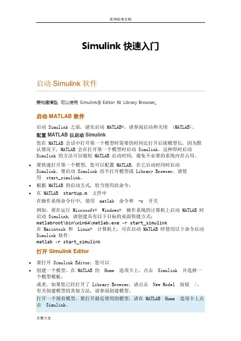
Simulink 快速入门要构建模型, 可以使用Simulink® Editor 和Library Browser。
启动 MATLAB 软件启动 Simulink 之前, 请先启动MATLAB®。
请参阅启动和关闭(MATLAB)。
配置 MATLAB 以启动 Simulink您在 MATLAB 会话中打开第一个模型时需要的时间比打开后续模型长, 因为默认情况下, MATLAB 会在打开第一个模型时启动 Simulink。
这种即时启动Simulink 的方法可以缩短 MATLAB 启动时间, 避免不必要的系统内存占用。
•要快速打开第一个模型, 您可以配置 MATLAB, 在它启动时同时启动Simulink。
要启动 Simulink 而不打开模型或 Library Browser, 请使用start_simulink。
•根据 MATLAB 的启动方式, 恰当使用此命令:•在 MATLAB startup.m文件中在操作系统命令行中, 使用matlab 命令和-r 开关例如, 要在运行Microsoft®Windows®操作系统的计算机上启动 MATLAB 时启动 Simulink, 请创建具有以下目标的桌面快捷方式:matlabroot\bin\win64\matlab.exe -r start_simulink在 Macintosh 和Linux®计算机上, 可在启动 MATLAB 时使用以下命令启动Simulink 软件:matlab -r start_simulink打开 Simulink Editor•要打开 Simulink Editor, 您可以:•创建一个模型。
在 MATLAB 的Home 选项卡上, 点击Simulink 并选择一个模型模板。
或者, 如果您已经打开了 Library Browser, 请点击New Model 按钮/。
有关创建模型的其他方法, 请参阅创建模型。

m精编b s i m u l i n k初级教程SANY标准化小组 #QS8QHH-HHGX8Q8-GNHHJ8-HHMHGN#Simulink仿真环境基础学习Simulink是面向框图的仿真软件。
演示一个Simulink的简单程序【例】创建一个正弦信号的仿真模型。
步骤如下:(1) 在MATLAB的命令窗口运行simulink命令,或单击工具栏中的图标,就可以打开Simulink 模块库浏览器(Simulink Library Browser) 窗口,如图所示。
图 Simulink界面(2) 单击工具栏上的图标或选择菜单“File”——“New”——“Model”,新建一个名为“untitled”的空白模型窗口。
(3) 在上图的右侧子模块窗口中,单击“Source”子模块库前的“+”(或双击Source),或者直接在左侧模块和工具箱栏单击Simulink下的Source子模块库,便可看到各种输入源模块。
(4) 用鼠标单击所需要的输入信号源模块“Sine Wave”(正弦信号),将其拖放到的空白模型窗口“untitled”,则“Sine Wave”模块就被添加到untitled窗口;也可以用鼠标选中“Sine Wave”模块,单击鼠标右键,在快捷菜单中选择“add to 'untitled'”命令,就可以将“Sine Wave”模块添加到untitled窗口,如图所示。
(5) 用同样的方法打开接收模块库“Sinks ”,选择其中的“Scope ”模块(示波器)拖放到“untitled ”窗口中。
(6) 在“untitled ”窗口中,用鼠标指向“Sine Wave ”右侧的输出端,当光标变为十字符时,按住鼠标拖向“Scope ”模块的输入端,松开鼠标按键,就完成了两个模块间的信号线连接,一个简单模型已经建成。
如图所示。
(7) 开始仿真,单击“untitled ”模型窗口中“开始仿真”图标,或者选择菜单“Simulink ”——“Start ”,则仿真开始。
第3章 SIMULINK简介及基本用法3.1 MATLAB语言简介研究和工作应用中都会遇到这样的困扰:当计算涉及矩阵运算或画图时,利用FORTRAN和C语言等计算机语言进行程序设计是一项很麻烦的工作,不仅需要对所利用的有关算法有深刻的了解,还需要熟练掌握所用语言的语法和编程技巧,并且对于一个并不复杂的计算任务,实现起来却十分枯燥繁琐,工作效率也不高.MATLAB正是为免除无数类似以上局面而产生的。
1980年前后,美国Cleve Moler博士在New Mexico大学构思开发了MATLAB(MATrix LABoratory矩阵实验室),它是集命令翻译、数值分析、矩阵运算、信号处理和图形显示于一体的一套交互式软件系统。
MATLAB最初由LINPACK和EISPACK计划研制,主要用于方便矩阵存取,其基本元素是无需定义维数的矩阵,经十几年完善扩充,现已发展为线性代数课程的标准工具,也成为许多领域课程的实用工具。
在工业环境中,MATLAB可用来解决实际的工程、数学问题,其典型应用有:通用的数值计算,算法设计,各种学科如自动控制、数字信号处理、统计信号处理等领域的专门问题求解。
3.2 Simulink简介3.2.1 Smulink介绍Simulink是MATLAB软件包之一,用于可视化的动态系统仿真,它适用于连续系统和离散系统,也适用线性系统和非线性系统。
它采用系统模块直观地描述系统典型环节。
因此可十分方便地建立系统模型而不需要花较多时间编程。
正由于这些特点,Simulink广泛流行,被认为是最受欢迎的仿真软件。
Simulink实际上是面向结构的系统仿真软件。
利用Simulink进行系统仿真的步骤是:(1)启动Simulink,进人Simulink窗口;(2)在Simulink窗口下,借助Simulink模块库,创建系统框图模样并调整模块参数;(3)设置仿真参数后,启动仿真;(4)输出仿真结果。
3.2.2 启动Simulink窗口及模型库用户首先进入MATLAB COMMAND窗口,键人Simulink,立即弹出Simulink模块库窗口,如图3-1所示。
Simulink的使用基础1.MATLAB的计算单元:向量与矩阵MATLAB作为一个高性能的科学计算平台,主要面向高级科学计算。
MATLAB的基本计算单元是矩阵与向量,向量为矩阵的特例。
一般而言,二维矩阵为由行、列元素构成的矩阵表示;对于m行、n列的矩阵,其大小为m×n。
在MATLAB中表示矩阵与向量的方法很直观,下面举例说明。
向量与矩阵⎥⎥⎥⎦⎤⎢⎢⎢⎣⎡=654C 例如,矩阵,行向量[1 2 3],列向量,在MATLAB中可以分别表示为⎥⎦⎤⎢⎣⎡=654321A >>A=[1 2 3; 4 5 6]>>B=[1 2 3]>>C=[4;5;6]注意:(1) MATLAB中所有的矩阵与向量均包含在中括号[]之中。
如果矩阵的大小为1×1,则它表示一个标量,如>>a=3%a表示一个数(2) 矩阵与向量中的元素可以为复数,在MATLAB中内置虚数单元为i、j;虚数的表达很直观,如3+4*i或者3+4*j 。
技巧:(1) MATLAB中对矩阵或向量元素的引用方式与通常矩阵的引用方式一致,如A(2 ,3)表示矩阵A的第2行第3列的元素。
如若对A的第2行第3列的元素重新赋值,只需键入如下命令:>>A(2,3)=8;则矩阵A变为A =1 2 34 5 8(2) MATLAB中分号(;)的作用有两点:一是作为矩阵或向量的分行符,二是作为矩阵或向量的输出开关控制符。
即如果输入矩阵或向量后键入分号,则矩阵与向量不在MATLAB命令窗口中显示,否则将在命令窗口中显示。
如输入矩阵>>A=[1 2 3; 4 5 6]% 按下Enter键,则在MATLAB命令窗口中显示 >>A =1 2 34 5 6(3) 冒号操作符(:)的应用。
冒号操作符在建立矩阵的索引与引用时非常方便且直接。
如上述对多维矩阵F的建立中,冒号操作符表示对矩阵F第一维与第二维所有元素按照其顺序进行引用,从而对F进行快速赋值,无需一一赋值。