FRAGSTATS_4.0教程
- 格式:pdf
- 大小:1.35 MB
- 文档页数:33

(完整word版)fragstats4.2基本教程Fragstats 4.2简易教程、使⽤说明1.数据格式Fragstats能够⽀持多种数据格式,但4.2以及后续版本将使⽤Geo TIFF grid作为主要的数据格式(图1)。
Data type selectionirr2.数据命名以及存放路径导⼊数据的名称和路径不能包含汉字和空格,且存放于⼆级⽬录,例如:D:\123\1987.tif3.背景问题背景值默认设置为999,但你完全可以在理解其意义的前提下依照⾃⼰喜好进⾏调整。
简单来说,背景即你分析过程中想要⾃动忽略的某种地表类型⼀⼀由于资料缺乏⽽⽆法归类、或者你单纯想将其作为背景值处理的地表类型。
值得注意的是,当设定为正值时,背景像元值被视作⽬标景观内部值;当设定为负值时,背景像元被视作⽬标景观外部值。
内部背景作为⽬标景观的⼀部分不仅会为整个景观⾯积作出贡献,并且会因此⽽改变许多指数值;外部背景不会被视作⽬标景观的⼀部分,只会对影像边缘的连接性产⽣影响。
在景观计算中,需要注意背景的影响。
这是景观指数误差中很⼤的⼀部分。
⽐如说,我们拿到的遥感图像,校正好后,边界裁剪后,⼀般不是规则的矩形。
在边边⾓⾓存在没有信息的像元。
图像分类后,没有信息的像元也是作为分类的⼀种的。
因此,需要对其进⾏去除。
这个操作可以在Arcgis下操作4.下载地址/doc/3a11f82f09a1284ac850ad02de80d4d8d05a01ff.html /la ndeco/research/fragstats/dow nloads/fragstats_d ownloads.html⼆、操作步骤2.1 打开Fragstats⾸先,从开始菜单或双击桌⾯图标打开Fragstats。
如果你的电脑上已安装10.0及以下版本的ArcGIS ,那么Fragstats打开时将有明显延迟(有时长达30s),这是由于Fragstats 在验证ArcGIS的使⽤许可(license )。


Fragstats 使用简单教程
我所使用的图像为快鸟简单分类影像,分辨率我重采样为 1 米,截取了一小块,格式为 erdasimg 格式主题影像。
类型数为 4,为了简单演示,并没有进一步操作。
图像的相关属性如下图所示
注意一般来说,在操作的时候 fragstats 建议忽略 0 值否则将会将 0 值算作一类来进行计算,
应该可以在背景值中进行设置。
在 erdas 中将其导出为 grid 格式(如下图所示)
就可以在 fragstats 中使用了 界面如下图所示
设置运行参数,下面简单描述一下参数设置面板
选择输入数据类型为 arcgrid 项 第一项 选择邻接规则和统计的水平 设置 grd 数据来源,输出文件位置,背景值设置为 o 值或极大数
接着确定后就可以回到主界面了
这是根据你所设置的运行统计水平就可以在工具条中选择各个水平的统计指标了如上图所 示
斑块水平
类型水平 上图
景观水平 上图
设置完成后 点击运行 见界面图说明 运行完成后弹出下面对话框 注意如果数据过大运行 速度将会比较慢,电脑可能会出现假死状态,请继续运行不要结束任务。
查看运行结果
结果如下图示
可以将结果另存为…在 excel 中导出
还要大家多试验,仅是抛砖引玉哦---------ateng-景观天下 地景版 /bbs/forumdisplay.php?fid=78&page=1 欢迎大家多支持本版发展
。


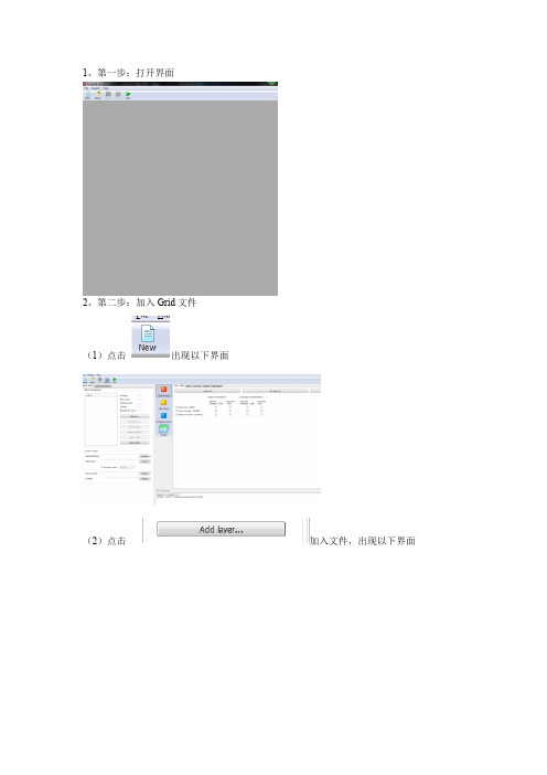
1、第一步:打开界面
2、第二步:加入Grid文件
(1)点击出现以下界面
(2)点击加入文件,出现以下界面
注意:加载文件的文件夹名称必须是英文字母一类的,不能出现中文,不然不能识别!
文件的格式就是ESRI的Grid的文件,Arcgis10.0即可完成该文件的转换。
(3)确保文件的有效性
竖行Y和横行X的数字必须有,且不是1和-1一类的,如果是的话那么就是错误的文件格式。
(4)选择计算类别
点击后出现
此步骤设置等与FR3.3基本类同。
(4)运行,点击后出现
(1)
(2)
(3)运行成功
如有ERROR出现则设置有
问题,需对应改正。
(4)点击查看结果
祝运用愉快,不懂的再问我。
广西大学林学院景观生态学作业
班级:林学171班姓名:黄靖杰学号:一.Fragstats软件的操作与运算:
1.打开Fragstats3.3。
2.点击Fragstats,选择Set Run Parameters,并在弹出的窗口设置运行参数并选择文件路径。
3.点击Fragstats,选择Select Land Metrics,在弹出的Land Metrics 窗口选择需要计算的指标,点击确定。
4.点击Fragstats,选择Select Class Metrics,在弹出的Class Metrics窗口选择需要计算指标,点击确定。
5.点击Fragstats,选择Execute开始运算。
6.点击Tools,选择Bowse Results查看结果。
结果如下图。
二.结果计算
1.按Save run as…导出软件运算结果
2.在文件管理器中将导出的“.land”、“.class”文件后缀名重命名为“.csv”
3.在excle中打开文件,通过公式运算得到结果
(1)景观优势度指数(landscape dominance index)
D=ln(5)-1.1952=0.4142
(2)景观均匀度指数(landscape evenness index)
E=1.1952 /ln(5)=0.7426。
概述什么是FRAGSTATSFRAGSTATS是空间格局的分析程序来表示景观结构的景观镶嵌模型分类地图。
请注意,FRAGSTATS不适合代表景观结构的景观梯度模型的连续表面地图。
景观受分析是用户定义的,并且可以表示任何空间的现象。
FRAGSTATS简单量化作为分类地图所代表的景观空间异质性;这是义不容辞的用户建立了良好的基础定义和缩放景观的主题内容和分辨率和空间的粮食和程度方面。
我们强烈建议您阅读使用该程序之前,FRAGSTATS背景部分。
重要的是,从FRAGSTATS输出才有意义,如果定义的景观是有意义的相对于正在审议的现象。
规模的注意事项FRAGSTATS需要的空间谷物或网格的分辨率是>0.001米,但它放置没有限制对景观本身的空间范围,虽然有对可加载的网格的尺寸存储器的限制。
然而,在计算FRAGSTATS的移动距离和面积为基础的度量报道平方米,公顷,分别。
因此,极端的程度和/或分辨率的景观可导致相当麻烦的数字和/或受舍入误差。
然而,FRAGSTATS输出,可以使用任何数据库管理程序,以重新调整指标或将其转换为其他单位(例如,转换公顷亩)被操纵以ASCII格式的数据文件。
计算机要求FRAGSTATS是一个用微软的Visual C单机+ +程序在Windows操作系统环境中使用,是一个32位进程(即使运行的是64位计算机上)。
FRAGSTATS的开发和在Windows 7操作系统上进行测试,尽管它应该在所有的Windows操作系统上运行。
请注意,FRAGSTATS是高度依赖于平台,因为它是在Microscroft环境下开发的,所以移植到其他平台上是不容易实现的。
FRAGSTATS是计算密集型的程序;其性能取决于两个处理器速度和计算机存储器(RAM)。
最后,处理的图像的能力依赖于足够的存储器可用,并且处理该图像的速度依赖于处理器速度。
特别值得注意的是该存储器的约束。
FRAGSTATS是一个32位的过程,因此,最多只能使用2GB的内存;但如果正确配置Windows可以让32位进程看高达3GB的内存。
Fragstats 4.2简易教程一、使用说明1.数据格式Fragstats能够支持多种数据格式,但4.2以及后续版本将使用Geo TIFF grid。
)作为主要的数据格式(图11图数据命名以及存放路径2.导入数据的名称和路径不能包含汉字和空格,且存放于二级目录,例如:D:\123\1987.tif背景问题3.但你完全可以在理解其意义的前提下依照自己喜好,背景值默认设置为999背景即你分析过程中想要自动忽略的某种地表类型——由进行调整。
简单来说,值得注于资料缺乏而无法归类、或者你单纯想将其作为背景值处理的地表类型。
当设定为负值时,背景像元值被视作目标景观内部值;意的是,当设定为正值时,内部背景作为目标景观的一部分不仅会为整个背景像元被视作目标景观外部值。
外部背景不会被视作目标景并且会因此而改变许多指数值;景观面积作出贡献,需要注意背景只会对影像边缘的连接性产生影响。
在景观计算中,观的一部分,比如说,我们拿到的遥感图像,的影响。
这是景观指数误差中很大的一部分。
在边边角角存在没有信息的像元。
边界裁剪后,一般不是规则的矩形。
校正好后,需要对其进行去除。
因此,没有信息的像元也是作为分类的一种的。
图像分类后,这个操作可以在Arcgis下操作。
4.下载地址/landeco/research/fragstats/downloads/fragstats_d ownloads.html二、操作步骤2.1打开Fragstats首先,从开始菜单或双击桌面图标打开Fragstats。
如果你的电脑上已安装10.0及以下版本的ArcGIS ,那么Fragstats打开时将有明显延迟(有时长达30s),这是由于Fragstats在验证ArcGIS的使用许可(license)。
请务必保持耐心(图2)。
2图 2.2新建模型一模型用于对斑块的景观结构进行分析。
接下来你需要创建一个Fragstats即为其配备了Fragstats进行了全副参数化,模型简单来说就是为个FragstatsNewFile按钮或从的下拉菜单中选择New分析所需的全部参数。
Last Updated: 28 May 2012Prepared by: Kevin McGarigalFRAGSTATS 4.0 TutorialThis tutorial is intended to provide FRAGSTATS users a "quick start" on how to use the software. All of the necessary data and files for the tutorial have been provided and these can be used as templates for how to format your own files latter on. However, this tutorial is not a substitute for the complete FRAGSTATS user manual; all serious FRAGSTATS users are responsible for understanding all of the information in the user manual.The tutorial is actually a series of short tutorials designed to demonstrate some of the basic features of FRAGSTATS; it is not intended to be a comprehensive guide, but rathera guide to help new users get started. The tutorials include the following:1.Setting Up Software and Inspecting Grids -- Covers the basic setup ofthe software and computer for running FRAGSTATS and an inspection of thegrids that will be used in the subsequent tutorials. All users should completethis tutorial.2.Analyzing a single grid -- Covers the essential steps involved in analyzinga single grid, including the use of ancillary tables for calculating functionalmetrics.3.Batch processing multiple grids -- Covers the use of batch files forprocessing multiple grids at once.4.Moving window analysis -- Covers the use of a moving window analysis tocreate local landscape structure gradients.5.Running the command line version from R -- Covers the execution ofFRAGSTATS command line version from R (programming environment andstatistical computing environment).Tutorial 1. Setting Up Software and Inspecting GridsIn this tutorial, we will setup the software and inspect the grids to be analyzed in the subsequent tutorials.1. Download and install FRAGSTATSFirst, if you haven't already done so, download FRAGSTATS 4.0 and run the setup utility to install the software on your computer.2. [Optional] Setup your Computer for use with ESRI ArcGISIf you intend to work with ascii or binary data formats, you can skip this step. However, if you have a valid ESRI ArcGIS license (version 10 or earlier) with Spatial Analyst or ArcView 3.3 Spatial Analyst and intend to work with ArcGrids (or Rasters), then there are two important requirements, as follows:First, you need to edit your computer system's environmental "path" variable. Specifically, FRAGSTATS must have access to the aigridio.dll library found in the “bin” (for ArcGIS installation) or the avgridio.dll library found in the “bin32" (for ArcView 3.3 installation) directory. Note, the paths may differ depending on your version and installation. Search your computer for the corresponding file and copy the path to the bin or bin32 directory, as appropriate. Note, the path does NOT include the aigridio.dll or avgridio.dll file name; it ends with bin or bin32. For example, for an ArcGIS 10 installation, the path might look like: C:\Program Files (x86)\ArcGIS\Desktop10.0\Bin The path to the corresponding bin directory should be specified in the windows system environmental variable, as follows:In Windows 7, the Environment variables can be accessed and edited from the Control Panel - System and Security - System - Advanced system settings under the “Advanced” tab and by clicking on “Environment Variables” (at the bottom of the dialog on the "Advanced" tab), as show in the figure below. In the list of System variables, select the “path” variable and select “edit” and add the path to the corresponding bin directory (e.g., ; C:\Program Files (x86)\ArcGIS\Desktop10.0\Bin). Note, you need a semicolon between each path in the list and make sure you enter the correct path on your system. If you are using a different Windows operating system, you'll have to figure out how to find the system environment variables, then edit the path variable as above.Second, you need to make sure that the ArcGrids that you intend to use, including those included with this tutorial, are located in a directory on your disk that does NOT contain any spaces in the full path. For example, if you have the tutorial grid reg78b located in the following directory:C:\Documents and Settings\Fragstats\Tutorial_1\reg78byou will get the following error message when attempting to Run FRAGSTATS: Error: Unexpected error encountered: [cannot_set_access_window for: C:\Documentsand Settings\Fragstats\Tutorial_1\reg78b]. Model execution halted.This is an irreconcilable problem with ESRI and the only solution is to put all your grids, including those included in this tutorial, in a directory that does NOT contain spaces. Note, this is probably good practice anyways, since there are other software programs that cannot deal properly with spaces in the path.3. Inspect the gridsNext, inspect the grids to make sure you understand the landscape definition before analyzing them, since the results of the analysis can only be interpreted in the context of the landscape definition.ArcGIS grids.--If you are planning on working with ESRI ArcGIS, open up the provided fragtutorial_1.mxd project in ArcMap. The project contains several data layers, as listed in the table of contents, including a landcover grid (lugrid) for an arbitrary extent in western Massachusetts.As you can see from the legend, the lugrid contains six landcover classes, including: 1) open (largely agriculture), 2) residential, 3) water (open water bodies and large rivers), 4) forest, 5) wetland, and 6) urban.Open the lugrid layer properties and inspect the grid properties on the Source tab. In particular, note the grid dimensions (1104 columns by 1035 rows), cell size (50 m), format (GRID), and pixel type (signed integer). The signed integer pixel type is necessary if the landscape has a border; i.e., strip of classified cells outside the landscape boundary and assigned negative class values. If the landscape does not contain a border, then an unsigned integer type is OK. In this case, the lugrid does not contain a border, but the sub-landscapes (below) do, so the pixel type has been set to signed integer.Next, open the lugrid layer attribute table and inspect the class values present on the grid. Note the class values and text description for each class. You will need to know the class values later on.Next, view the reg78b grid by selecting it in the table of contexts and zooming to the layer extent. This grid is a randomly selected roughly 5x5 km (25 km2) square sub-landscape sampled from the lugrid. Expand the legend and note the landcover classes present; it has the same six landcover classes as before, but with the addition of six "border" classes.The border is simply a strip of classified cells surrounding the landscape of interest that provides information on patch type adjacency along the landscape boundary. In the legend provided, the border classes have been assigned a lighter shade of the color assigned to the corresponding class inside the landscape boundary. Importantly, a border is identified in FRAGSTAST by negatively valued cells. An inspection of the grid attribute table reveals the same six landcover classes as before, but with both a positive (inside the landscape boundary) and negative (border, or outside the landscape boundary) version of each class. Note, I created all three of the grids in this project containing borders (reg78b, reg66b and reg21b) using the fragborder.aml script provided. This aml (arc macro language) is executed from the arc prompt and requires ArcInfo Workstation. Briefly, the script clips the lugrid layer with a polygon coverage for one of the sub-landscapes, and then buffers the polygon by 50 m and clips the lugrid layer again but with the buffered (i.e., slightly larger) polygon. Next, the larger grid is multiplied by -1 to convert the cell values to negative. Lastly, the two grids are merged, with the smaller grid (the sub-landscape of interest) on top, resulting in positive valueseverywhere except the narrow strip of cells in the border.Lastly, view the other sub-landscape grids in the table ofcontents. There are three different sub-landscapes: reg78,reg66, and reg21, each of which also contains a versionwith a landscape border: reg78b, reg66b, and reg21b.These landscape differ largely in the amount of forestlandcover.Ascii/binary grids.--If you are planning on workingwith ascii or binary grids, open up the provided files in atext editor and inspect them. Ascii files are interpretable,binary files are not. Neither are pretty to look at and youcan't do much with them, but it is useful to know whatthese files look like.Open up reg78b2.asc in a text editor (the top left portionof this file is shown below). This a space-delimited asciifile (i.e., there is a space between each cell entry) and istherefore interpretable. Note, this ascii file was created byconverting the reg78b ArcGrid to an ascii file in ArcMap.Note the header information included in the first six linesof the file. This header information must be deleted before it can be analyzed in FRAGSTATS; however, the information on the grid dimensions (ncols=102 andnrows=102) and cellsize (50) will be needed later when parameterizing the FRAGSTATS model. In particular, note the landscape border indicated by the negative class values in the first row and column.Viewing the ascii grids is a bit more difficult without importing them into your favorite GIS. However, if you are an R user, you can use the following script (or open theprovided script, tutorial-1.R) to plot the grid in R. Note, there are several ways to plot the grids in R. If you are familiar with the Raster package, you can import the ascii grids and plot them quite easily, but specifying a color scheme for the legend and plotting a pretty legend is a bit tricky. The following script makes use of the base functions in the Graphics library:First, set the working directory to wherever you have installed the tutorial; e.g.: setwd('c:/work/fragstats/software/fragstats4/tutorial/tutorial_1')Next, read in the ascii grid, as a matrix, into an object (m):m<-as.matrix(read.table('reg78b.asc'))Next, in order to assign colors to each landcover class, identify each unique class value: uv<-sort(unique(as.vector(m)))Next, create breaks for assigning colors to class values (breaks are at the minimum -1, midpoints and maximum +1). Note, this is necessary because the plot function (image) is designed for continuous variables not categorical variables as is the case with the landcover image:my.breaks<- (c(min(uv)-2, uv) + c(uv, max(uv)+2 ))/2Next, create a color legend for the plot:my.colors<-c('gray','lightskyblue','lightgreen','lightpink','lightyellow','yellow', 'purple','slateblue','green','skyblue','black')Next, check to make sure you have a color for every unique class value:if(length(my.colors) != length(uv)) stop("You need a color for every unique value")Next, print to the console the color associated with each class value to verify that you have what you want:data.frame(code=uv, color=my.colors)Finally, plot the image with the image() function in the graphic library. Note, because image() does a 90 degree counter-clockwise rotation of the image, a matrix transpose and some indexing is necessary to rotate the image back to its original orientation:image(t(m)[,nrow(m):1],asp=1,breaks=my.breaks,col=my.colorsTutorial 2. Analyzing a Single GridIn this tutorial, you will compute a suite of structural and functional patch, class and landscape metrics for a single input grid.1. Open FRAGSTATSFirst, open FRAGSTATS from the start menu orby double clicking on the FRAGSTATS icon onthe desktop. Note, if you have an ESRI ArcGIS10 installation, there may be a significant delay(up to 30 seconds in some cases) in opening theuser interface as FRAGSTATS tries to secure avalid ArcGIS license, so be patient -- and don'tforget to thank ESRI for their licensemanagement while you're waiting.If FRAGSTATS does not open or you get a runtime initialization error or any other kind of error, it probably means that you have ArcGIS installed on your machine and there is problem securing a valid license for Spatial Analyst. If you are sure that you followed the installation instructions and/or followed the instructions in Tutorial #1 step 2, then download the Diagnostic Tool from the FRAGSTATS website and after extracting the utility from the zip file, run the utility and copy the report and submit it in an email to mcgarigalk@.Note, if you have ArcGIS installed on your machine, but either you don't have a valid Spatial Analyst license or you simply don't want to run FRAGSTATS with ArcGrids, then be sure that your system's environmental "path" varible does NOT contain a path to ArcGIS. If your system's path variable contains ArcGIS, FRAGSTATS thinks you are an ArcGIS user and that you want to use ArcGrids, and it tries to secure a valid Spatial Analyst license. Unfortunately, to use FRAGSTATS in this situation, you will have to remove ArcGIS from your system's path variable.2. Create a New modelNext, you need to create a FRAGSTATS "model" for a categorical landscape representing the patch mosaic model of landscape structure. A FRAGSTATS model is simply a file containing a complete parameterization of FRAGSTATS; i.e., everything needed to conduct an analysis. Click on the New button on the tool bar or select New from the File drop-down menu. This creates a blank model for you to parameterize.3. Import a gridNext, import a grid to analyze. Specifically, you need to Add a layer to the batch manager on the Input layers tab. Click on the Add layer button to open the import datadialog.If you are using ESRI ArcGIS, you can select the ESRI grid data type in the left pane and then navigate to the tutorial directory by clicking on the [...] button and selecting the reg78b grid. Note, when you load an ArcGrid, the grid attribute informationpertaining to row count (y), column count (x) and cell size are read from the grid headeritself, and thus these fields are grayed out in the dialog. The only grid attribute item that you need worry about (and can modify) is the background value. By default the background class value is set to 999, but you can change it here to any class value that you want, so long as you understand the implications. Briefly, background is a class used to distinguish cells that you essentially want to ignore in the analysis; these can be cells that couldn't be classified to a real landcover class for lack of data, or cells that you simply want to treat as part of the background matrix in the landscape. To fully understand the implications of designating background, be sure to read the help files on backgrounds, borders, and boundaries in the section on User guidelines - Overview. For now, keep the background value set to 999.If you are using ascii or binary files, you can select the corresponding data type in the left pane and then navigate to the tutorial directory by clicking on the [...] button and selecting the corresponding grid. For example, to use the provided ascii grid, selectreg78b.asc. Note, when you try to load an ascii grid or binary grid, the grid attribute information must be entered manually. If you don't enter this information before selecting the grid, the software will complain that the layer attributes are invalid, so be sure to enter valid numbers for each of the attributes after selecting the grid. Specifically, for this grid, you need to enter row count (y) = 102, column count (x) = 102, and cell size = 50. As with ArcGrids, you can also edit the background class value, but for now, keep the default value of 999.4. Optionally, input a class descriptors tableNext, you have the option of inputting a class descriptors table. The class descriptors table allows you to specify a character description (i.e., patch type) for each numeric class value, specify whether to compute statistics for each class, and whether to designate each class as background. The class descriptors table is optional. If you do not provide this table, then the numeric class values are used in the output, all classes are enabled and none are treated as background except any class with the assigned background value (999 in this case).Open up the provided descriptors.fcd file in a text editor. Note, FRAGSTATS recognizes .fcd as the extension for class descriptor files, but this is not a required extension. This file contains four fields. ID refers to the numeric class values; these are the unique cell values in the grid. These values derive from your landscape definition. Name is simply a description of each class and this will be output as TYPE in the FRAGSTATS output files. Enabled is a logical (true or false) and indicates whether to compute and output statistics for the corresponding class. Lastly, IsBackground is logical (true or false) and indicates whetherto treat each class as background or not.Note, a "true" involves reclassifying thecorresponding class to the backgroundvalue specified earlier (999 in this case). Ifwe had specified say, 400, as thebackground value earlier, then Water wouldbe treated as background regardless of whatis designated in this table.To use the provided class descriptors file, click on the Class descriptors Browse button in the Common tables section of the user interface on the Input layers tab and navigate to the tutorial directory and select the descriptors.fcd file.5. Specify additional parameters for the analysisNext, you need to specify some additional parameters for the analysis. Click on the Analysis parameters tab on the left pane of the user interface. Here, is where you chose the neighbor rule for delineating patches (4 cell rule or 8 cell rule) and specify whether you want to analyze the conventional multi-level structure of the landscape or assess local landscape structure gradients via moving window analysis.For this tutorial, keep the default 8 cell neighbor rule and select the Multi-level structure [tabular output]; the local structure gradient via moving window (grid output) is covered in tutorial #4. In addition, check the boxes for Patch, Class and Landscape metrics. Note, you must have at least one of the these boxes checked or you will get an error message later when trying to run the model. However, only check the level corresponding to the metrics you want to compute. Some applications will involve patch level metrics, for example when evaluating the spatial character and context of each habitat patch in a metapopulation context. Other applications will involve only the class level metrics, for example when evaluating the fragmentation of a focal class. And still other applications will involve only the landscape level metrics, for example when evaluating overall landscape heterogeneity. Of course, some applications will involve more than one level of metric.6. Select metricsNext, you need to select some metrics to compute. Give that you selected patch, class and landscape metrics in step 5, you need to select individual metrics at each of these levels.To begin, select Patch metrics in the top right pane of the user interface. Click on the Patch metrics button and then on each tabbed set of metrics. You can chose a subset of metrics or simply "Select all" -- your choice. Note, on the Aggregation tab, if you select either the Proximity index or the Similarity index, then you also need to specify a Search radius. These metrics are "functional" metrics and thus require additional parameterization. Both of these metrics require a search radius; the Similarity index also requires a similarity weights table (see below). To specify a search radius, click on the [...] button and enter the desired search radius in meters; e.g., 500.Next, click on the Class metrics button and then on each tabbed set of metrics. Again, you can chose a subset of metrics or simply "Select all" -- your choice. Note, on the Area-Edge tab, if you select Total Edge or Edge Density, then you need to consider how you want to treat any background or boundary edge in the edge calculations. The default is to not consider any of it as true edge. However, you can chose to treat all of it as edge or any specified proportion as edge. To change the default, click on the [...] button and enter your choice. Note, since the input landscape contains a border and does not contain any designated background, the issue is mute since we know the true status of every edge segment along the landscape boundary and there are no background edges to worry about. Similarly, on the Aggregation tab, if you select the Connectance index, then you also need to specify a threshold distance within which patches are deemed "connected". Simply click on the [...] button and enter the desired threshold distance in meters; e.g., 500.Lastly, click on the Landscape metrics button and then on each tabbed set of metrics. Again, you can chose a subset of metrics or simply "Select all" -- your choice. Note, on the Diversity tab, if you select Relative Patch Richness, then you also need to specify the maximum number of classes (or patch types). Simply click on the [...] button and enter the value; 6 in this case.7. Conditionally, input additional common tablesNext, if you selected any of the Core area metrics, Contrast metrics or Similarity index (on the Aggregation tab) at any level (patch, class or landscape), then you also need to create and input additional ancillary tables in order to parameterize these metrics. If you fail to input these tables or try to input improperly formatted tables, you will get an error message and the analysis will fail. Importantly, it is up to you to create these ancillary files to ensure that they are meaningful to your application. There are nomeaningful default values for these tables; creating these tables is how you functionalize the corresponding metrics for your particular application.Open up the provided edgedepth.fsq file in a text editor. Note, FRAGSTATS recognizes .fsq as the extension for these common ancillary tables, but this is not a required extension. This comma-delimited ascii file contains the depth-of-edge effect distances (in meters) for each pairwise combination of classes (or patch types). The file must begin with the line: FSQ_TABLE. It can contain any number of comment lines beginning with the character symbol #. It must contain a class list of literal names (i.e., class descriptors) or numeric class values corresponding exactly to those in the class descriptors file. Note, only one of these lists is required and if both are provided, as in the example below, only the first one encountered is used. Note, the list should include a item for every class in the input grid. If the list contains additional classes not found in the input grid, they are simply ignored. Similarly, if the list omits a class found in the input grid, the edge depths are assumed to be zero by default.The class list is followed by the edge depths for each pairwise combination of classes, given in the order they are provided in the list, and is read as follows. The row indicates the focal class and the column indicates the adjacent class. Thus, the fourth row is for Forest (fourth in the list) as the focal class, and each of the entries represents the depth-of-edge effect distance penetrating into Forest from an adjacent class. For example, in the table below, Open has an edge effect that penetrates 100 m into Forest, Resident penetrates 50 m into Forest, and so on. Note, in this example, edge effects are specified only for the Forest class.To use the provided edgedepth file, click on the Edge depth Browse button in the Common tables section of the user interface on the Input layers tab and navigate to the tutorial directory and select the edgedepth.fsq file.Repeat the process above for the provided contrast.fsq and similarity.fsq tables; these tables provide the edge contrast weights and similarity coefficients for each pairwise combination of classes (patch types), respectively.8. Optionally save the modelNext, you might want to save the model for future use. Often times it is easier to open a saved model and modify it than to create a new model from scratch. At any point in the process of parameterizing the model, simply click on the Save or Save as buttons on the toolbar or select these options from the File drop-down menu to save the model. Simply navigate to the desired directory and enter a file name for the model. Note, FRAGSTATS will automatically assign the extension .fca to the file, which identifies the file as a model for a categorical landscape.9. Run the modelNext, you are ready to run the model. Simply click on the Run button on the toolbar or select this option from the Analysis drop-down menu. This will open the Run dialog that lists the number of metrics selected at each level (patch, class and landscape). If you like what you see, click on the Proceed button, otherwise click on Cancel and make the needed modifications to the model. In the example shown here, the run includes 75 patch metrics, 109 class metrics and 116 landscape metrics because I selected All the available metrics at each level.10. Browse the resultsPay attention to the Activity log in the bottom right pane of the user interface. If all went well, you will learn that the run ended and how long it took. Assuming that the run wassuccessful, you are now ready to browse the results. Click on the Results button in the top-right pane of the user interface and then on each tabbed set of results. The results are displayed in a table for each level of metrics selected. So, if you computed patch, class and landscape metrics, as was done here, there will be results in each of the corresponding tabs. Otherwise, only the tab corresponding to the level of metrics computed will contain data; the others will be empty. The Patch tab will contain a row for each patch in the input landscape and a column for each patch metric selected. The Class tab will contain a row for each (non-background) class in the input landscape and a column for each class metric selected. The Landscape tab will contain a single row for the entire input landscape mosaic and a column for each landscape metric selected.Once you have verified that the tables contain results, the next step is probably to export the tables so that you can use them in subsequent analyses. To export the results, simply click on the desired run in the Run list (note, at this point you should have only one run listed), and then click on Save run as... and navigate to the desired folder and enter a basename for the output files. The basename will be given an extension corresponding to each level of metrics computed (basename.patch, basename.class, and nd). Thus, in this example, three files will be created corresponding to the three levels of metrics computed. Note, a fourth output file containing the cell adjacency information can be created by checking the Save ADJ file check box (basename.adj). Each of these output files is a comma-delimited ascii file and can easily imported into other software such as R and Excel for further analysis and summary.Note that is also possible to automatically save the results with the execution by checking the Automatically save results option on the Analysis parameters tab in。