Advanced SeqMonk
- 格式:pdf
- 大小:987.38 KB
- 文档页数:35

七鳃鳗属3种类的亲缘关系分析CHANG Yu-mei;HUANG Jing;SUN Bo;SU Bao-feng;LIANG Li-qun【摘要】对来自中国、俄罗斯和美国的北极七鳃鳗L.camtschaticum COI部分序列82条、俄罗斯的溪七鳃鳗L.reissneri 17条和中国的朝鲜七鳃鳗L.morii3条,共计102条进行亲缘关系和系统进化分析,以明确七鳃鳗属Lethenteron3个种类的分类地位和亲缘关系.单倍型检测发现,北极七鳃鳗共有14种单倍型,其中中国群体4种,俄罗斯群体11种,美国群体3种,大部分个体共享2种单倍型;溪七鳃鳗有3种单倍型,均与北极七鳃鳗共享;朝鲜七鳃鳗辽宁丹东群体和黑龙江抚远群体各独享1种单倍型.系统进化分析显示,除了朝鲜七鳃鳗黑龙江群体Hap16单独聚类外,其余15种单倍型无明显分化,聚为一支.单倍型序列分歧检测发现,黑龙江群体Hap16无论种内或种间,均与其他15种单倍型分歧达到种级(~2%)分化水平.因此,推测朝鲜七鳃鳗黑龙江群体为七鳃鳗属一个有效种,溪七鳃鳗为北极七鳃鳗的不同生态类型.【期刊名称】《水产学杂志》【年(卷),期】2018(031)006【总页数】6页(P12-17)【关键词】七鳃鳗属;COI基因;系统进化【作者】CHANG Yu-mei;HUANG Jing;SUN Bo;SU Bao-feng;LIANG Li-qun 【作者单位】【正文语种】中文【中图分类】S917七鳃鳗(Lamprey)是现存的古老无颌类脊椎动物的代表种,是脊椎动物演化发育生物学研究的重要模式动物。
全球有3科(七鳃鳗科Petromyzonidae、地蝗科Geotriidae和水螨科Mordaciidae),10属,超过40种。
其中4种隶属于南半球的地蝗科和水螨科,而其余种都属于北半球的七鳃鳗科[1,2]。
七鳃鳗属Lethenteron隶属于七鳃鳗科,主要分布在欧亚大陆[3]。

For more details see how the Advanced Permissions for Magento 2 extension works.Guide for Advanced Permissions for Magento 2Provide limited access to your store management for different admin users. Benefit from advanced role permissions to let specific managers work with particular products, categories, product attributes, websites, and store views.Limit access by store view or websiteControl access to product and categories managementRestrict access to product attributesEnable selective dashboard accessLimit access to CMS pagesCreating Roles with Advanced PermissionsPlease make sure you have created the required user before assigning a new role with advanced permissions. You can learn how to add new users here.To create a new sub-admin role with advanced permissions, please navigate to Admin panel →System → Permissions → User Roles. Then, hit the Add New Role button.Role Information and Resources1.Specify the Role Name;2.Switch to the Role Resources tab;3.Change the Resource Access option to Custom;4.Specify the resources this role will have access to.You can provide user role with extra privileges under the System → Amasty Role Permissions branch of the tree.Please hit the Save Role button and open this role again to have the ability to assign the new role to users.Then, you can assign this role to certain users. Click the Role Users tab and flag the required users. Setting Advanced PermissionsWith the extension, you can set up advanced permissions to provide or limit access for your store managers to the certain parts of the admin panel. It is possible to restrict the access to a dashboard and CMS elements by limiting website/store view access.Advanced: ScopeIn this tab you can limit access to certain store views or websites. Modify the Limit Access To option to:Allow all stores;Limit certain websites;Limit certain store views.For the websites and store views option you should specify the required ones.If you limit user's access to a particular store view or a webstore, the access to a dashboard and CMS pages of this webstite/store view will be limited automatically as well.For the website and store views options you can limit user role access to the following parts of yourstore:Orders;Invoices and Transactions;Shipments;Credit Memos.Select between the Yes or No options.Advanced: CategoriesIn the Categories tab you can provide this role with access to all product categories or limit to selected categories. Please tick the necessary categories or subcategories to allow access to them. See how a user with a particular role sees a category tab:Advanced: ProductsNext, the Products tab enables you to provide access to all, only selected, or own created products. In second case you will need to flag the required product.As a result, a particular user will get access to the selected products only.In third, you can make products accessible only for their owners that is convenient for the multi-vendor stores.If the user hasn't created any products yet, the grid will remain empty.But, if the user creates a product, it becomes visible and available for editing.Please see this part of the guide to know how to set product owners. Advanced: Product AttributesIn the Product Attributes tab you can restrict access to certain product attributes. Set the Allow Access To option to Selected Attributes and specify the desired attributes for this user role. Advanced: Admin User RoleFinally, in the Admin User Role tab you can allow this user to create the new users with the selectedroles. Choose the appropriate option from the dropdown menu and select the required roles. Please make sure that you enabled the User management option and disabled the Role management option for this role in the Role Resources tab.When the configuring of a certain user role is done, hit the Save Role button.Creating Sub-Admin UsersIf you need to add extra users to your admin panel, please go to System → Permissions → All Users and hit the Add New User button.Specify account information and switch to the User Role tab. From here you can tick the desired radio-button to provide this user with certain administrative privileges. When done, hit the Save User button.Return to the previous steps to know how to set up a user role with advanced permissions. Changing Product OwnerTo provide selective access to a certain product you can set up its owner.1.Go to Products → Catalog;Select the desired product;2.3.Specify product owner in the drop-down menu.Make sure that you switched the Advanced: Products option to Own Product Only option.FAQ* Is it possible to create a user that can only see and edit one product attribute?* The user I created cannot add or edit products, even though I ticked the Products > Inventory > Products checkboxes. How to solve that?* Is it possible to only allow a user view and edit specific customer attributes in the customer profile? * Is it possible to only give a user access to specific customers/customer groups?* Show more articles →Find out how to install the Advanced Permissions extension via Composer.。
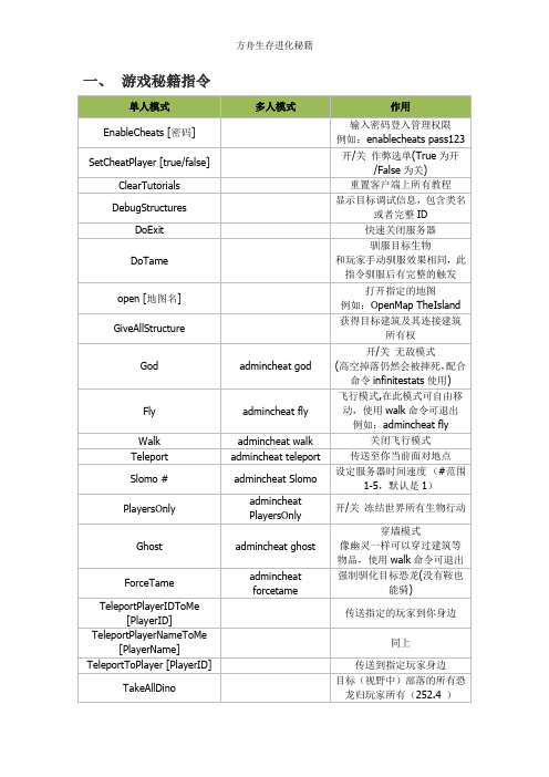
一、游戏秘籍指令二、499道具物品ID配合秘籍 GiveItemNum 使用示例:giveitemnum 105 10 1 false //获得物品ID为105的小存储箱10只(注意:多人模式下使用 admincheat GiveItemNum 命令)。
三、观察者模式激活观察者模式后按以下键位:四、物品品质关于制造物品指令GiveItemNum [ID] [数量] [品质] [图纸1成品0]参数中出现的物品品质物品的品质,其实指的是物件的等级,和动物等级相似,等级越高,物件就越强越耐用,也越棒。
这些物件的质素分类为6级,如下:1)Primitive:最初级,代表色是灰色2)Ramshackle:初级,代表色是绿色3)Apprentice:中级,代表色是蓝色4)Journeyman:中高级,代表色是紫色5)Mastercraft:高级,代表色是黄色6)Ascendant:最高级,代表色是红色五、恐龙代码配合秘籍 Summon 使用。
注意:多人模式下使用admincheat summon 命令示例:召唤甲龙 Summon Ankylo_Character_BP_C六、恐龙蓝图配合秘籍 SpawnDino 使用。
秘籍示例:SpawnDino"Blueprint'/Game/PrimalEarth/Dinos/Lystrosaurus/Lystro_Character_BP.L ystro_Character_BP'" 1 1 1 120 //获得一个120级的水龙兽七、道具物品蓝图配合秘籍 GiveItem秘籍示例:GiveItem"Blueprint'/Game/PrimalEarth/CoreBlueprints/Items/Armor/Shields/Prima lItemArmor_WoodShield.PrimalItemArmor_WoodShield'" 1 0 0注意: 1、多人模式下使用 admincheat giveitem 命令 2、注意分号的用法。

Stratix 5700Industrial Managed Ethernet SwitchThe wide deployment of EtherNet/IP™ in industrial automation means that there is a growing demand to manage the network properly.Integtrating new machine-level networks into an existing plant network requires convergence.With more devices connected on the same Ethernet network than ever before, an industrial managed switch can help you simplify your network infrastructure. Adding a managed switch to your network architecture can also help make the process of adding new machines easier. The Allen-Bradley® Stratix 5700™ is a compact, scalable Layer 2 managed switch with embedded Cisco technology for use in applications with small isolated, to complex networks. With integration into Studio 5000 Automation Engineering and Design Environment™, you canleverage FactoryTalk® View faceplates and Add-on Profiles for simplified configuration and monitoring.By choosing a switch co-developed by Rockwell Automation and Cisco, your Operations Technology (OT) and Information Technology (IT) professionals leverage tools and technology that are familiar to them. This collaboration can also help to reduce configuration time and cost.Features and Benefits:Advanced Networking Features• Integrated Device Level Ring (DLR) connectivity helps optimize the network architecture and provide consolidated network diagnostics • Integrated Network Address Translation (NAT) provides 1:1 IP address mapping helping to reduce commissioning time • Power over Ethernet (PoE) versions provide power to devices over Ethernet minimizing cabling • Security features, including access control lists, help ensure that only authorized devices, users and traffic can access the network • Secure Digital (SD) card provides simplified device replacementOptimized integration:• Studio 5000® Add-on Profiles (AOPs) enable premier integration into the Rockwell Automation Integrated Architecture® system • Predefined Logix tags for monitoring and port control • FactoryTalk® View faceplates enable status monitoring and alarming • Built-in Cisco® Internet Operating System (IOS) helps provide secure integration with enterprise networkDesigned and Developed for EtherNet/IP Automation ApplicationsNetwork Address TranslationMachine integration onto a plant network architecture can be difficult as machine builder IP-address assignments rarely match the addresses of the end-user network. Also, network IP addresses are often unknown until the machine is being installed. The Stratix 5700 with Network Address Translation (NAT) is a Layer 2 implementation that provides “wire speed” 1:1 translations ideal for automation applications where performance is critical.NAT allows for:• Simplified integration of IP-addressmapping from a set of local,machine-level IP addresses to theend user’s broader plant network• OEMs to deliver standard machinesto end users without programmingunique IP addresses• End users to more simply integratethe machines into the larger network192.168.1.4192.168.1.4MACHINE 1MACHINE 2Private Network Private NetworkSwitch Reference ChartAllen-Bradley Stratix 5700 Industrial Ethernet SwitchSwitch Selection TableFE - Fast Ethernet GE - Gigabit EthernetPublication ENET-PP005F-EN-E – April 2016Copyright ©2016 Rockwell Automation, Inc. All Rights Reserved. Printed in USA.Supersedes Publication ENET-PP005E-EN-E – March 2015EtherNet/IP is a trademark of the ODVA.Cisco is a trademark of Cisco Systems, Inc.Allen-Bradley, CompactLogix, Factory Talk, Integrated Architecture, Kinetix, LISTEN. THINK. SOLVE., Powerflex, Rockwell Automation, Rockwell Software, Stratix 5700, Studio 5000, Studio 5000 Automation Engineering and Design Environment are trademarks of Rockwell Automation, Inc.Glossary of TermsAccess Control Lists allow you to filter network traffic. This can be used to selectively block types of traffic to provide traffic flow control or provide a basic level of security for accessing your network.CIP port control and fault detection allows for port access based on Logix controller program or controller mode (idle/fault). Allows secure access to the network based on machine conditions.CIP SYNC (IEEE1588) is the ODVAimplementation of the IEEE 1588 precision time protocol. This protocol allows very high precision clock synchronization across automation devices. CIP SYNC is an enabling technology for time-critical automation tasks such as accurate alarming for post-event diagnostics, precision motion and high precision first fault detection or sequence of events.Device Level Ring (DLR) allows direct connectivity to a resilient ring network at the device level.DHCP per port allows you to assign a specific IP address to each port, confirming that the device attached to a given port will get the same IP address. This feature allows for device replacement without having to manually configure IP addresses.Encryption provides network security by encrypting administrator traffic during Telnet and SNMP sessions.EtherChannel is a port trunking technology. EtherChannel allows grouping several physical Ethernet ports to create one logical Ethernet port. Should a link fail, the EtherChannel technology will automatically redistribute traffic across the remaining links.Ethernet/IP (CIP) interface enables premier integration to the Integrated Architecture with Studio 5000 AOP , Logix tags and View Faceplates.FlexLinks provides resiliency with a quick recovery time and load balancing on a redundant star network.IGMP Snooping (Internet Group Management Protocol) constrains the flooding of multicast traffic by dynamically configuring switch ports so that multicast traffic is forwarded only to ports associated with a particular IP multicast group.* Separate SW IOS requiredKey Software FeaturesMAC ID Port Security checks the MAC ID of devices connected to the switch to determine if it is authorized. If not the device is blocked and the controller receives a warning message. This provides a method to block unauthorized access to the network.Network Address Translation (NAT) provides 1:1 translations of IP addresses from one subnet to another. Can be used to integrate machines into an existing network architecture.Port Thresholds(Storm control & Traffic Shaping)allows you to set both incoming and outgoing traffic limits. If a threshold is exceeded alarms can be set in the Logix controller to alert an operator. Power over Ethernet (PoE) provides electrical power along with data on a single Ethernet cable to end devices.QoS – Quality of Service (QoS) is the ability to provide different priority to different applications, users, or data flows, to help provide a higher level of determinism on your network.REP (Resilient Ethernet Protocol) – A ring protocol that allows switches to be connected in a ring, ring segment or nested ring segments. REP provides network resiliency across switches with a rapid recovery time ideal for industrial automation applications.Smartports provide a set of configurations to optimize port settings for common devices like automation devices, switches, routers, PCs and wireless devices. Smartports can also be customized for specific needs.SNMP Simple Network Management Protocol (SNMP) is a management protocol typically used by IT to help monitor and configure network-attached devices.Static and InterVLAN Routing bridges the gap between layer 2 and layer 3 routing providing limited static and connected routes across VLANs.STP/RSTP/MST Spanning Tree Protocol, is a feature that provides a resilient path between switches. Used for applications that requires a fault tolerant network.VLANs with Trunking is a feature that allows you to group devices with a common set of requirements into network segments. VLANs can be used to provide scalability, security and management to your network.802.1x Security is an IEEE standard for access control and authentication. It can be used to track access to network resources and helps secure the network infrastructure.。

SequenceManagerLogix Controller-based Batch and Sequencing SolutionA Scalable Batch Solution for Process Control ApplicationsA modern batch system must account for the growing need for architecture flexibility, true distribution of control, and scalability. SequenceManager software provides batch sequencing in the Logix family of controllers by adding powerful new capability closer to the process and opening new possibilities for skids, off network systems, and single unit control. SequenceManager allows you to configure operations in Studio 5000 Logix Designer®, run sequence in FactoryTalk® View SE, and to capture and display batch results.SequenceManager directs PhaseManager™ programs inside a Logix-based controller in an ordered sequence to implement process-oriented tasks for single unit or multiple independent unit operations. Using industry standard ISA-88 methodology, SequenceManager enables powerful and flexible sequencing capabilities that allow for the optimal control of sequential processes.With SequenceManager, you can deliver fast and reliable sequence execution while reducing infrastructure costs for standalone units and complete skid-based system functionality.Key BenefitsSequenceManager™ software significantly reduces engineering time for system integrators and process equipment builders while providing key controller-based batch management capabilities for end users. Key benefits include:• Enables distributed sequence execution • Fast and excellent reliability of sequence execution native to controller • Efficient sequence development and monitoring in core product • Integrated control and HMI solution for intuitive operation • Reduced infrastructure costs for small systems • Provides data necessary for sequence reportingDistributed Batch Management Based on Proven TechnologyBuilt Upon Rockwell AutomationIntegrated ArchitectureSequenceManager was built using the standard control and visualization capabilities found in Rockwell Automation® Integrated Architecture® software. SequenceManager is a new capability that is builtinto Logix firmware that uses visualization through FactoryTalk® View SE to create an integrated sequencing solution. Combined with event and reporting tools, SequenceManager software is a complete batch solution for single unit and skid-based process applications.Scalable Controller-based Solution SequenceManager allows flexible design for skid-based equipment to be developed, tested and delivered asa fully functioning standalone solution but, if needed, seamlessly integrated into a larger control system. This strategy provides the end user with the option to integrate equipment without imposing design constraints on the OEM delivering the skid. Additionally, it enables the end user to deliver equipment as a standalone system without the constraint to scale to a larger process solution in the future. This batch solution offers scalability to help prevent costly redesign and engineering.Flexibility to Meet Process Needs SequenceManager enables you to expand your process control on skid based equipment that performs repetitive tasks and decision-making abilities. By using the ISA-88 methodology, SequenceManager allows for control design that can be adopted to fit the needs of the process industries without the constraints of custom application code. Built-in state model handling provides for fast and easy configuration while maintainingcontrol of the process.Editor and ViewerAs a brand new program type in Studio 5000 Logix Designer®, SequenceManager™ software gives the user the power and flexibility necessary to create dynamic recipes to maximize the effectiveness of the process control system.Without limitations on steps and parameters, and the ability to run parallel phases, to branch, and to loop back and rerun steps, SequenceManager removes the barriers in achieving effective batch within the controller.Sequence ExecutionProcedural sequences are executed through nativefunctions in the controller. With an integrated ISA-88 state model, the control and states of phases can be assured. Standard batch functionality, such as manual control and active step changes, are included to give the operational flexibility that is needed to respond toabnormal process conditions.Allowing for an Intuitive Batch ApplicationResponsive batch interactions between the controller and equipment, along with intuitive operator interfaces, provide the core of a truly distributed batching strategy that drives ISA-88 procedural models.Allen-Bradley, FactoryTalk Batch, FactoryTalk® View SE, Integrated Architecture, Listen.Think.Solve., PhaseManager, PlantPAx, Rockwell Automation, Rockwell Software, SequenceManager, and Studio 5000 Logix Designer are trademarks of Rockwell Automation, Inc. Trademarks not belonging to Rockwell Automation are property of their respective companies.Operator ViewerFactoryTalk® View SE and ActiveX controls monitor and interact with a running procedural sequence through the HMI. Advance ActiveX controls provide an intuitive interface for controlling sequences and changingparameters from the operational environment. Improved capabilities allow the user to perform manual step changes and acquire control easily.Reporting and AnalyticsSequenceManager data generates events that are used to produce batch reports and procedural analysis. A separate event client transfers the event data from the Logixcontroller to a historical database. SequenceManager uses the same data structure and reports as FactoryTalk Batch, which provides a consistent and intuitive batch reporting tool among Rockwell Automation® Batch Solutions.Additional InformationVisit us at /processPublication PROCES-PP001A-EN-E – June 2016Copyright © 2016 Rockwell Automation, Inc. All Rights Reserved. Printed in USA.。

dnbc4tools的调用摘要:1.DNBC4Tools简介2.DNBC4Tools的安装与配置3.DNBC4Tools的主要功能与使用方法4.实战案例:如何使用DNBC4Tools进行数据处理5.总结与建议正文:尊敬的读者,您好!在这篇文章中,我们将介绍一款功能强大的数据处理工具——DNBC4Tools。
本文将详细阐述DNBC4Tools的安装与配置、主要功能及使用方法,并通过实战案例帮助您更好地理解和应用这款工具。
最后,我们将给出一些总结与建议,以期能够帮助您在实际工作中发挥DNBC4Tools的最大作用。
1.DNBC4Tools简介DNBC4Tools是一款为生物信息学研究人员设计的数据处理工具,主要用于处理大规模的Next Generation Sequencing(NGS)数据。
这款工具集成了多种功能,包括质量控制、数据过滤、比对、转录组分析等,能够为研究者提供一站式的解决方案。
2.DNBC4Tools的安装与配置在安装DNBC4Tools之前,请确保您的计算机已安装Python 3.x。
接下来,按照以下步骤进行安装:(1)打开终端或命令提示符,输入以下命令:```pip install dnbc4tools```(2)等待安装完成。
安装完成后,您需要配置DNBC4Tools的环境变量。
请按照以下步骤操作:(1)打开DNBC4Tools的安装目录,找到`dnbc4tools.py`文件。
(2)在该文件所在的目录下,创建一个名为`.dnbc4tools`的文件夹。
(3)在`.dnbc4tools`文件夹中,创建一个名为`config.py`的文件,并输入以下内容:```config = {"data_dir": "path/to/your/data/directory","reference_genome": "path/to/your/reference/genome","output_dir": "path/to/your/output/directory","tools_dir": "path/to/your/tools/directory"}```请将上述路径替换为您实际的数据、参考基因组、输出和工具目录。
松墨天牛转铁蛋白基因克隆及生物信息学分析蔡紫玲;刘琪司;林同【摘要】转铁蛋白是一类非血红素结合铁的β1-球蛋白,广泛分布于脊椎动物和无脊椎动物体内.克隆了松墨天牛转铁蛋白基因(登录号:KU213914),命名为MaTf,其核苷酸序列全长为2 549 bp,包含一个2 178 bp的开放阅读框(ORF)和一个371 bp的带有加尾信号的3'非编码区(3'UTR).采用生物信息学方法分析MaTf的编码蛋白,结果显示:松墨天牛转铁蛋白分子量约为80 ku,等电点为7.36,为稳定蛋白,有信号肽,不含跨膜结构域,有1个糖基化位点,有平均分布在整条肽链的43个磷酸化位点.二级结构多为随机卷曲,仅有21.52%α螺旋,24%β片层(延伸链)结构,能形成三段卷曲螺旋,为亲水性蛋白,N端和C端各有1个TR_FER结构域.【期刊名称】《广东农业科学》【年(卷),期】2016(043)004【总页数】7页(P117-123)【关键词】松墨天牛;转铁蛋白;生物信息学;结构域【作者】蔡紫玲;刘琪司;林同【作者单位】华南农业大学林学与风景园林学院,广东广州510642;华南农业大学林学与风景园林学院,广东广州510642;华南农业大学林学与风景园林学院,广东广州510642【正文语种】中文【中图分类】S476.9;Q789蔡紫玲,刘琪司,林同.松墨天牛转铁蛋白基因克隆及生物信息学分析[J].广东农业科学,2016,43(4):117-123.松墨天牛(Monochamus alternatus)是毁灭性病害松材线虫(Bursaphelenchus xylophilus)的主要媒介昆虫,也是松树的重要蛀干害虫。
松墨天牛的寄主植物多为松属(Pinus)植物,包括黑松(Pinus thunbergii)、马尾松(Pinus massoniana)、云南松(Pinus yunnanensis)、赤松(Pinus densiflora)等[1],也可危害冷杉属(Abies)、黄杉属(Pseudotsuga)、落叶松属(Larix)、铁杉属(Tsuga)和雪松属(Cedrus)等[2]。
AdvancedSkeleton高级骨骼插件基本介绍(2011-02-08 22:34:12)转载▼分类:教程标签:杂谈AdvancedSkeleton高级骨骼插件基本介绍这个插件的基本功能还是不错的,目前版本到了3.0了吧,后面会陆续地介绍一些常用的插件,如:TSM、TFM、zootoolbox等等……1.简介:AdvancedSkeleton Pro是Maya的角色设计的工具的合集。
主要特点是:Pro不再局限于预先设计好的FitSkeleton,而是可以创建任意的FitSkeleton;具有本地旋转轴和旋转度,并可控;可以从AdvancedSkeleton 回到FitSkeleton,方便你做些改变然后重建AdvancedSkeleton;Pro在身体配置方面不再做限制,三个头,五条腿,100个手指都可以;支持拖拽“Selector Designer",可以通过拖曳的方式创建自定义的选择界面。
同时,“PoserDesigner”可以创建、保存和使用姿势。
2. 安装运行安装文件(setup.exe)选择目标目录注意: 安装目录要设置在本地磁盘我的文档下例如:C:\Documents and Settings\Name\My Documents\Maya\2008\完成安装。
启动Maya现在你就可以在工具栏里看到一个叫“advancedSkeleton”的部分3. 概述:AdvancedSkeleton 的关键功能是:由一个简单的骨骼链(FitSkeleton)生成一个复杂的运动系统(AdvancedSkeleton)因为在角色的右边,所以关节是朝向负X方向的并且会被镜像到角色的左边以下这些信息都是从FitSkeleton关节中读取的:名字、位置、旋转、旋转轴向、旋转The following information gets read from the FitSkeleton从这个关节也可以决定高级的控制器,如:标签和输入和输出的连接关系图以下的关节标签会创建高级控制器:并且不局限于设置驱动关键帧,任何可以连接上的节点都可以。
国外站点magento2.1.1.3 网站安装步骤修改日期:2018-9-7作者:吴立星QQ:376819879一、安装前部署(带产品案例的网站的框架包)1)PHP 7.0.12版本、MYSQL 5.6.0版本、2)运行版本php7.0.12+nts+apache3)修改配制文件修改内容如下:未打开的请去除”;”符号(extension=php_openssl.dllextension=php_intl.dllsys_temp_dir = "/tmp" 注意:这里需要在盘符里新增文件夹D://phpStudy/tep soap.wsdl_cache_dir="/tmp"memory_limit 128M更改为512M,max_execution_time 30更改为1800 (此项时间)max_allowed_packetextension_dir="D:\phpStudy\php\php-7.0.12-nts\ext" 确认有此目录)3)新增日志目录安装过程的文件5)安装插件6)在MY SQL 里新增空数据库如:magento2113(后续需要用到数据库名称)二、安装过程1)安装过程中保证网络正常,请勿断网;如出现卡在3%、4% 、64% 、68% 超过半小时的(已超最大限时),可以重新运行安装,程序会自动从中断过程中恢复安装2)安装时提示后台地址(如果非首次安装一定修改到本次安装目录地址)3)安装成功提示:1. 2.3. 4.5. 6.7.8.9.成功后及可以看到前台与后台前台。
advancedmarkerelement用法全文共四篇示例,供读者参考第一篇示例:AdvancedMarkerElement是一种用于在软件中标记数据的高级元素。
它可以帮助用户更有效地管理和处理复杂的数据,提高工作效率和数据分析能力。
在本文中,我们将深入探讨AdvancedMarkerElement的用法,并介绍如何在实际工作中运用它来处理数据。
二、AdvancedMarkerElement的用法1. 标记数据:通过AdvancedMarkerElement,用户可以将数据标记为不同的类别或类型。
这样可以帮助用户更容易地识别出数据中的重要信息,并据此作出相应的决策。
2. 分类和归类:AdvancedMarkerElement可以帮助用户对数据进行分类和归类,从而更好地组织和管理数据。
这有助于用户更有效地对数据进行分析和整理。
3. 过滤和筛选:用户可以利用AdvancedMarkerElement对数据进行过滤和筛选,从而找出符合特定条件的数据。
这有助于用户更快速地从海量数据中找到所需要的信息。
4. 数据关联和统计:AdvancedMarkerElement还可以帮助用户分析数据之间的关联性,便于用户对数据进行综合分析和统计。
这对于用户了解数据之间的联系和趋势非常有帮助。
第二篇示例:AdvancedMarkerElement是一个常用的Vue.js插件,它为开发者提供了更加方便和高效的方式来处理标记元素。
在本文中,我们将介绍AdvancedMarkerElement的用法以及如何在Vue.js项目中使用它。
一、什么是AdvancedMarkerElement```npm install advancedmarkerelement```安装完成后,我们可以在Vue组件中引入AdvancedMarkerElement并使用它。
以文本标记为例,我们可以使用如下代码创建一个简单的文本标记:```html<template><div><AdvancedMarkerElement type="text" text="这是一个文本标记"/></div></template>在这个例子中,我们通过引入AdvancedMarkerElement来创建一个文本标记,其中type属性指定了标记类型为文本,text属性指定了标记的内容为“这是一个文本标记”。
Advanced Analysis with SeqMonkVersion 1.3.0Advanced SeqMonkLicenceThis manual is © 2012-2014, Simon Andrews.This manual is distributed under the creative commons Attribution-Non-Commercial-Share Alike 2.0 licence. This means that you are free:∙to copy, distribute, display, and perform the work∙to make derivative worksUnder the following conditions:∙Attribution. You must give the original author credit.∙Non-Commercial. You may not use this work for commercial purposes.∙Share Alike. If you alter, transform, or build upon this work, you may distribute the resulting work only under a licence identical to this one.Please note that:∙For any reuse or distribution, you must make clear to others the licence terms of this work.∙Any of these conditions can be waived if you get permission from the copyright holder.∙Nothing in this license impairs or restricts the author's moral rights.Full details of this licence can be found at/licenses/by-nc-sa/2.0/uk/legalcodeIntroductionOnce you have been working with SeqMonk for a while you will quickly master the basic controls and plots. The real trick to making effective use of the program though is how you apply the tools you have to your data.This course is intended as a follow on to the basic SeqMonk course and goes into some of the more advanced features of the program, as well as providing some advice on how the tools can best be applied to your data. This course focusses more on handling biases within your data and how to apply more rigorous statistical analyses –including those applicable to more complex experimental designs such as time courses or dose responses.As with the original course I’ve tried to keep the advice here as neutral as possible with regard to a ny specific type of experiment. The topics presented here should be of use for the analysis of most kinds of data since they address generic problems from sequencing experiments.Data ImportWhilst basic data import is hopefully pretty simple, there are a few additional options which you may not have tried and which might make life easier.Reimporting DataRather than importing data from a mapped file you can reimport it from the current SeqMonk project or a different project.Cross Importing DataTo cross-import data from a different SeqMonk project you can select File >Import Data > SeqMonk Project. This will then check to see that thegenome assemblies match between the other project and your currentproject and will then find the list of DataSets in the project from which youcan select those you wish to import. You can copy over as many or as fewas you like into your current project.Reimport within the same projectYou can also choose to reimport a dataset youalready have in your current project. This willduplicate the data in the project, but also allowsyou to select some of the other import options atthe same time. Modifications you can make whenre-importing would include deduplication,extension, or reversing the strand of all reads.You can also filter the re-imported data either bykeeping or rejecting reads which overlap with aclass of features, or by more generally down-sampling the data to keep a random subset ofwhat you started with.HiC ImportOne of the newest features in SeqMonk is the ability to handle HiC association data. HiC data comes as pairs of reads, where there is no expectation that the reads sit physically close together, or are even on the same chromosome. Analysis is based on the degree of association of parts of the genome based on the number of pairs of reads whose ends come from the regions being compared.HiC import is now a standard option from any of the import tools. There is no special format for HiC data, but the import filter assumes that all of the data comes in pairs of HiC associated positions. This means that to create a mapped HiC file you should only include sequences where both ends were mapped and the mapped positions should be placed immediately after one another in whichever file format you choose to use.There is very little SeqMonk can do to check that your HiC data was correctly formatted, so if you have mismatched your sequences you are unlikely to see an error from the program. The best way to check whether the data is OK is to run a HiC heat map following import to see what you get. Heat maps should produce a characteristic pattern, and if your data seems to be randomly distributed then you should be suspicious that the data import failed.During HiC import there are some options you can apply to filter the data as it comes in. For the most part filtering is better done at an earlier stage during mapping using programs such as HiCUP, however some filtering can be applied at import. Specifically you can choose to remove short interaction pairs, or you can choose to ignore trans hits (pairs which sit on different chromosomes) to significantly reduce the size of your dataset if you’re specificall y looking at cis interactions.Automatic sample groupingAfter importing data into SeqMonk you should create appropriate sample groups and replicate sets to group your samples together. The two are used for different purposes:∙Data Groups merge the raw data for two or more data sets and make them appear as if they had been imported from a single file.∙Replicate Sets average the quantitation for two or more data sets or groups, but retain the distribution of quantitated values for use in statistical tests. Replicate sets should be used to mark biological replicates of each experimental condition.Although you can make data groups and replicate sets manually using the options under the data menu, there is a quicker way to create them if your data set names have a consistent naming scheme using the option Data > Auto Create Groups/Sets.In the box on the left you can put in a set of text strings which can be found in the names of your data sets and which mark the groups you want to create. The tool will then look for a match to each string and will make either a data group or a replicate set out of the samples which match. If you need to use more than one discontinuous string match to define your groups then you can separate strings with bar characters to make more complex patterns. Groups made this way can always be edited with the traditional data group and replicate set editors.Quantitation PipelinesThe traditional way to quantitate data in SeqMonk is to use a two step process where the first step involves the creation of a set of probes over regions which will later be quantitated, and the second step assigns a value to each probe for each dataset based on the data.In some cases there are types of quantitation which can’t be performed in this type of 2-step process, and there are also some common quantitations for which it would be convenient to have a simpler way to perform them. These use cases are what Quantitation Pipelines were designed for. They are automated quantitation processes which can perform probe generation, quantitation and potentially even filtering in a single step. Quantitation pipelines can be accessed under Data > Quantitation Pipelines.RNA-Seq quantitation pipelineThe RNA-Seq pipeline uses a type of quantitation which can only be perfomed within a pipeline since it requires that quantitation and probe generation are performed simultaneously. The basic premise of the pipeline is that it is a read count quantitation over a set of features, but for multi-exon features it only counts the reads which sit over the exons of the feature and ignores those in the introns.The options you have within the pipeline allow you to choose which class of features you’re going to use to quantitate your data (see the later notes about filtering features based on their biotypes). You can also choose the type of strand specificity in the libraries you’re quantitating so you can only count the relevant reads.The default quantitation from this pipeline is log2 RPM (reads per feature per million reads of library), but you can alter this. If you’re going to use the quantitation in an external analysis tool such as DESeq or EdgeR then you will need uncorrected raw read counts, so there is an option to generate these. If you want to compare the expression levels of different genes within the same sample then you can also correct by read length to get log2 RPKM values, but this is not recommended when comparing expression values between samples.By default the RNA-Seq pipeline merges together the exons of different transcript isoforms for the same gene to give you a single per-gene expression value. You can choose to get output for each transcript isoform by unticking the ‘merge transcript isoforms’ box, but SeqMonk does not try to do a likelihood based assignment of reads to a single isoform, so reads which map against more than one isoform will be counted more than once in this mode.Wiggle plot pipelineThe wiggle plot pipeline is a convenience method, and everything in this pipeline could be performed in the normal quantitation options. This simply generates a set of running window probes and quantitates them with a corrected read count. This is an easy way to generate an initial unbiased quantitation of your data to look quantitatively at your read counts over a region of interest.You can choose which region you want to analyse (just what you’re looking at now, the current chromosome or the whole genome) and the pipline will try to select a suitable window size for your probes.Bisulphite methylation over featureWhen analysing bisulphite data what is imported into SeqMonk are not the read positions, but the individual methylation calls. In a BS-Seq dataset each ‘read’ is only 1 base long and the strand of the read indicates the methylation state (forward = methylated, reverse = unmethylated).You can calculate a percentage methylation value for a region of the genome by simply counting the total number of methylated and unmethylated calls within that region, however this has a number of problems. You could have very few calls which could result in a very unreliable overall methylation value. You could also have very biased coverage such that the majority of your reads come from one or two positions within the region which again might not produce a good overall average.The bisulphite methylation pipeline provides a way to account for some of these problems. It provides a way to filter each call position by the degree of coverage and then produces an overall methylation value which weights each valid call position equally. It also uses a flag value to mark those positions for which an overall level of methylation could not be determined reliably.Splicing efficiency quantitation pipelineThe splicing efficiency quantitation pipeline generates a measure of splicing efficiency for RNA-Seq datasets. The basic premise for the pipeline is that samples which exhibit lower splicing efficiency will have a greater proportion of reads in their introns. The pipline therefore quantitates features based on the density of reads in introns and exons. You can then use these values to look for overalldifferences in splicing between samples, or to find individual transcripts where this might have changed.Antisense transcription pipelineThe antisense transcription pipeline again operates on RNA-Seq data, but is specifically designed for data coming from directional libraries. The aim of the pipeline is to identify putative regions which are undergoing antisense transcription.The pipeline performs both a quantitation and a statistical analysis of a set of genes. It first looks for the genome wide level of antisense transcription to get an idea of how ‘leaky’ the strand specificity is across the whole library. In a second pass it then analyses each gene individually to see how many reads were found on the sense and antisense strands. It uses a binomial test to see if the number of antisense reads is unexpectedly high, and quantitates the gene with an obs/exp value. As well as producing a quantitation the pipeline also makes a probe list for each sample listing the significantly antisense genes it identified.NormalisationSeqMonk provides a series of tools to quantitate your raw data. These include some normalisation options allowing you to correct for factors such as the total number of reads in your dataset and the length o f the probe you’re quantitating. Although this initial quantitation can provide useful data, in many cases it is susceptible to other sources of bias which might cause systematic differences between your datasets, and which might lead you to make incorrect conclusions about the differences between your data.Common sources of bias might be:∙Having greatly different numbers of reads between samples, meaning that low values may be measured with very different accuracies between data sets.∙Having different levels of PCR duplication between samples∙Having different read lengths∙Having different total amounts of signal between samples (eg RNA-Seq samples where there is more transcription in one sample than another.∙Having different degrees of mis-mapping contaminating sequences into different samplesBefore you trust your quantitation you should therefore take some time to look at the set of quantitated values you have produced and compare these between your datasets. If there are systematic differences between your samples then you either need to think of why this might make sense biologically, or if you decide the differences are technical you can try to normalise the data so that their influence is removed.Cumulative distribution plotThe easiest way to visualise and compare the distribution of values you have between your datasets is to use the cumulative distribution plot. This plot simply shows you the path your quantitated data takes to get from the lowest value in your set to the highest. Different datasets which show the same distribution of values (even if individual measures show large changes) should have virtually identical paths on this plot, and the aim of normalising data is to make the paths as similar as possible.At the low end of this plot you will see some instability and stepping of the plot due to very low absolute counts. In some data sets you will clearly see separate points for probes with 1, 2, 3 etc reads in them. As the absolute counts increase the plot will tend to smooth out, but this may happen at different points in different datasets depending on their coverage levels.Empty ValuesOne of the biggest problems when dealing with count based data are places where you saw no data at all. The problem is that because you saw nothing you can have no idea how much more sequencing you would have had to have performed until you saw some data in that position. Comparing an empty probe to one with a small amount of data (especially when there is a difference in the total amount of data collected) is very problematic, and one of the largest causes of false predictions in this type of data.The problem of empty values is exacerbated when the quantitation values are log transformed. Since you can’t log transform a zero value you have to assign some arbitrary value to it to allo w it to have a real value after transformation. The problem is further compounded by adding corrections for length and total counts, and at what stage the small value is added to allow log transformation.In the end the compromise made by SeqMonk is that if count data is to be log transformed then any empty values are given a raw count of 0.9. This applies to both the read count quantitation where 0.9 of a read is added, and to the base pair quantitation where 0.9 of a base is added. Any transformations for probe length and total count are then applied on top of this initial value.In practice this has some consequences for empty probes in your data.1. If you log transform and correct for probe length then your empty probes will have differentabsolute values within a dataset. This makes some kind of common sense since finding no reads in a probe which is 10kb long should not necessarily be viewed the same as finding no reads in a probe with is 10bp long. In extreme cases you may observe a small secondary distribution of empty probes to the left of your probe value distribution, but mostly these will tend to blend in with the bottom end of the very lowly measured reads.2. If you log transform your data and correct for total read count then empty probes will not haveexactly the same value between datasets. The values will be consistent within a dataset (if you haven’t corrected for probe length), but you may incorrectly think you have real changes occurring between probes which are empty in both sets if y ou aren’t careful about your filtering criteria.Whilst this way of handling empty reads isn’t absolutely ideal it is the best compromise we can come up with, and in most cases will produce sensible results. The only condition where this will give very misleading results will be cases where you have very large differences in the total number of reads between datasets such that the proportion of empty probes varies wildly. Even in these cases the other normalisation techniques described here should identify and help to correct this problem, but in general you need to stay aware of the accuracy with which your measurements are being made.Removing outliersOne obvious source of bias is the presence of outliers in your data. Many of the quantitation methods used in NGS analysis apply some kind of correction for the total number of sequences in the dataset. The assumption made is that the general distribution of sequences over the genome is similar between datasets and that you can scale the actual counts you got up or down to match the total number of sequences in each dataset.There are a few problems with this assumption. One of the major problems is that we tend to assume that all of the genome is represented in our current genome assembly. Whilst many genomes have very good assemblies they still have large holes over specific regions, and these can cause problems. In particular telomeric and centromeric regions are very large (and indeed variable in length), and are almost completely unrepresented in the assemblies due to their highly repetitive nature. However sequences from these regions will still turn up in our libraries. This wouldn’t be a problem if our mapping programs caused them never to be mapped to the genome, but what we see instead is that some proportion of this extra sequence is mapped incorrectly to a position within the genome assembly. These incorrect mapping positions then show huge enrichment, even in unbiased or control samples, and the huge number of counts from these mismapped sequences can have an influence on the global count corrections which are applied. In the plot below, which shows read counts on a log scale – the single top outlier covers only 1:500000th of the genome, but contains 4.5% of all of the reads.As an example of this, if you have a look at the distribution of read counts over a genome you will tend to see a strong upward spike in read counts at the ends of many of the chromosomes. This spike results from incorrectly mapped reads coming from the repetitive s equence which isn’t part of theassembled genome. The classic example of where you see this is the Sfi1 gene in human/mouse which has many of these repeats in it, and consequently is often predicted as having a significant biological effect, when actually it’s a victim of incorrect normalisation.In addition to the generic problem of repeats, some techniques will specifically enrich for a specific class of repeats, and an increased mismapping ratio for these sequences will produce a global bias in the normalisation. MeDIP samples, for example, often enrich major satellite sequences which can comprise up to 40% of all sequences in the library. These are generally absent from the assembly, and can thus produce a small number of strong mismapped peaks, which can contain up to 20% of all mapped sequences.One way around this problem is to simply remove extreme outliers before performing your final quantitation. The outliers we’re talking about here will have an enrichment level way in excess of anything which could be produced by a ChIP or RNA-Seq enrichment and could only realistically be derived from mapping artefacts. Typically they will have read counts two or three orders of magnitude above the rest of the distribution and can be removed by a simple values filter. If you have an input sample which you expect to show an even distribution then you can use the box-whisker filter with a harsh filter to find these mismapping events globally and remove them.Once you have filtered your original probe list to remove these aberrant regions then you need to use the ‘Existing Probe List Probe Generator’ to promote the filtered list up to being a full probe set which you can then re-quantitate. When re-quantitating you need to ensure that you only count reads within the probe set when correcting for total read count.Percentile normalisationA commonly observed pattern, especially on ChIP and other enrichment based libraries, is that your distributions follow a similar path, but on a somewhat different scale. Thus the original quantitation would suggest that there is a consistent difference between your samples, and scatterplots would show an off-diagonal consistent relationship between the samples. This kind of discrepancy can be caused by a change in the proportion of reads falling into the probes being measured, either through mismapping, or through a change in the efficiency of the ChIP enrichment. Since the differences observed do not in most cases represent an actual biological change then it is reasonable to aim to normalise away this difference.The simplest tool to achieve this type of normalisation is the Percentile Normalisation Quantitation. This quantitation method allows you to set a reference percentile in your data and the existing quantitations will have a correction factor applied to them such that their values at your chosen percentile will match exactly. Normally it makes sense to set the reference percentile to somewhere around 75% since this will be in the well measured portion of your data, but before any big changes which might occur at the extreme end of the distribution.You can also choose what kind of correction will be applied. The default is an additive correction where a constant value is added to each point to get the distributions to match. The downside to this method is that the same correction will be applied everywhere, and will end up with different values being set for the empty probes in your different data sets. A more appropriate correction in these cases is to use a multiplying factor to correct your data. This will ‘stretch’ your distribution to match at the specified percentile and may more closely match the overall distributions, especially at the low end.Since the same correction is applied to all points on your distribution this is a fairly safe and uncontentious correction to apply, but in some cases this correction alone will not be enough to completely match the distributions of your samples.Matching distributionsIf you have found some variation in the distributions of your samples which you are unable to satisfactorily remove using the total read correction, length correction or percentile normalisation correction then the ultimate way of making your distributions match is to use the Match Distribution quantitation method. This method makes up an averaged distribution from all of your current samples, and then forces all of your individual distributions to follow this average distribution exactly. You will therefore end up with perfectly matching distributions (or at least as close as your measurement resolution will allow – the method will not cause probes which previously had the same value to have different values).You can think of this method of normalisation as being similar to the ‘Convert to ranks’ normalisation method, which simply removes all of the quantitation from your data, and gives a value to each probe simply based on its position between the lowest and highest values. In this case we do something similar, but instead of putting the values on a straight line from lowest to highest, we follow the average trajectory which the original values took, thereby preserving any gross features in the distribution.Performing this kind of normalisation is more risky than something like the percentile normalisation because it does not treat every probe equally. It forces all samples onto the same distribution whether or not that makes biological sense. You therefore need to be sure that you’re definitely not interested in whatever differences you are using this method to remove. For example it would be completely inappropriate to normalise both the input and ChIP samples from a ChIP-seq experiment this way, since the input would be expected to show a much flatter distribution than the enriched sample, however normalising several ChIPs from the same antibody might be more justified. In other samples it might be valid to use this to normalise RNA-Seq samples which had different coverage and had then had to be deduplicated, since these will show an intensity dependent bias, but it would be bad touse this to match up distributions between RNA-Seq samples which had different overall amounts of transcription.It would also be bad to use this on enrichment samples where there was truly a biological reason for the different amount of enrichment. An extreme example of this would be the case of a ChIP vs and input sample, where you’d expect the input to be much flatter, and the ChIP to show a wider dynamic range.In any case, the match distribution normalisation should be the last step in your normalisation protocol, and you should try to match your distributions as closely as possible using the other methods mentioned before using this, since otherwise some samples will have much more influence over your averaged distribution than others.Manual normalisationFor some specialised applications it may be that the information you need to correctly normalise your data isn’t present in the mapped sequences themselves. Most sequencing application s are by their nature relative measures, telling you what proportion of reads fall into a particular gene, but not how this relates to an absolute measure in your original sample. To take a simple example, two RNA-Seq datasets taken from samples where the distribution of transcripts were identical, but the absolute level of transcription was different, would look exactly the same in the mapped data. Only by incorporating some external measure could you account for this type of difference.To allow you to apply these kinds of correction SeqMonk has a manual correction option. This lets you enter a manual correction value for each of your datasets and choose how this is applied to the set of quantitated values calculated by SeqMonk. By using this option you can incorporate absolute external measures with the relative measures the program itself can produce.Normalising to other samplesIn some cases you might want to normalise your samples against each other - quantitating sample A as the difference between sample A and sample B for example. There is a quantitation module which lets you apply this type of more complex normalisation called the relative quantitation module.。