Surface Reconstruction with Triangular B-splines

Screened Poisson Surface ReconstructionMICHAEL KAZHDANJohns Hopkins UniversityandHUGUES HOPPEMicrosoft ResearchPoisson surface reconstruction creates watertight surfaces from oriented point sets.In this work we extend the technique to explicitly incorporate the points as interpolation constraints.The extension can be interpreted as a generalization of the underlying mathematical framework to a screened Poisson equation.In contrast to other image and geometry processing techniques,the screening term is defined over a sparse set of points rather than over the full domain.We show that these sparse constraints can nonetheless be integrated efficiently.Because the modified linear system retains the samefinite-element discretization,the sparsity structure is unchanged,and the system can still be solved using a multigrid approach. Moreover we present several algorithmic improvements that together reduce the time complexity of the solver to linear in the number of points, thereby enabling faster,higher-quality surface reconstructions.Categories and Subject Descriptors:I.3.5[Computer Graphics]:Compu-tational Geometry and Object ModelingAdditional Key Words and Phrases:screened Poisson equation,adaptive octree,finite elements,surfacefittingACM Reference Format:Kazhdan,M.,and Hoppe,H.Screened Poisson surface reconstruction. ACM Trans.Graph.NN,N,Article NN(Month YYYY),PP pages.DOI=10.1145/XXXXXXX.YYYYYYY/10.1145/XXXXXXX.YYYYYYY1.INTRODUCTIONPoisson surface reconstruction[Kazhdan et al.2006]is a well known technique for creating watertight surfaces from oriented point samples acquired with3D range scanners.The technique is resilient to noisy data and misregistration artifacts.However, as noted by several researchers,it suffers from a tendency to over-smooth the data[Alliez et al.2007;Manson et al.2008; Calakli and Taubin2011;Berger et al.2011;Digne et al.2011].In this work,we explore modifying the Poisson reconstruc-tion algorithm to incorporate positional constraints.This mod-ification is inspired by the recent reconstruction technique of Calakli and Taubin[2011].It also relates to recent work in im-age and geometry processing[Nehab et al.2005;Bhat et al.2008; Chuang and Kazhdan2011],in which a datafidelity term is used to“screen”the associated Poisson equation.In our surface recon-struction context,this screening term corresponds to a soft con-straint that encourages the reconstructed isosurface to pass through the input points.The approach we propose differs from the traditional screened Poisson formulation in that the position and gradient constraints are defined over different domain types.Whereas gradients are constrained over the full3D space,positional constraints are introduced only over the input points,which lie near a2D manifold. We show how these two types of constraints can be efficiently integrated,so that we can leverage the original multigrid structure to solve the linear system without incurring a significant overhead in space or time.To demonstrate the benefits of screening,Figure1compares results of the traditional Poisson surface reconstruction and the screened Poisson formulation on a subset of11.4M points from the scan of Michelangelo’s David[Levoy et al.2000].Both reconstructions are computed over a spatial octree of depth10,corresponding to an effective voxel resolution of10243.Screening generates a model that better captures the input data(as visualized by the surface cross-sections overlaid with the projection of nearby samples), even though both reconstructions have similar complexity(6.8M and6.9M triangles respectively)and required similar processing time(230and272seconds respectively,without parallelization).1 Another contribution of our work is to modify both the octree structure and the multigrid implementation to reduce the time complexity of solving the Poisson system from log-linear to linear in the number of input points.Moreover we show that hierarchical point clustering enables screened Poisson reconstruction to attain this same linear complexity.2.RELA TED WORKReconstructing surfaces from scanned points is an important and extensively studied problem in computer graphics.The numerous approaches can be broadly categorized as follows. Combinatorial Algorithms.Many schemes form a triangula-tion using a subset of the input points[Cazals and Giesen2006]. Space is often discretized using a tetrahedralization or a voxel grid,and the resulting elements are partitioned into inside and outside regions using an analysis of cells[Amenta et al.2001; Boissonnat and Oudot2005;Podolak and Rusinkiewicz2005], eigenvector computation[Kolluri et al.2004],or graph cut [Labatut et al.2009;Hornung and Kobbelt2006].Implicit Functions.In the presence of sampling noise,a common approach is tofit the points using the zero set of an implicit func-tion,such as a sum of radial bases[Carr et al.2001]or piecewise polynomial functions[Ohtake et al.2005;Nagai et al.2009].Many techniques estimate a signed-distance function[Hoppe et al.1992; 1The performance of the unscreened solver is measured using our imple-mentation with screening weight set to zero.The implementation of the original Poisson reconstruction runs in412seconds.ACM Transactions on Graphics,V ol.VV,No.N,Article XXX,Publication date:Month YYYY.2•M.Kazhdan and H.HoppeFig.1:Reconstruction of the David head ‡,comparing traditional Poisson surface reconstruction (left)and screened Poisson surface reconstruction which incorporates point constraints (center).The rightmost diagram plots pixel depth (z )values along the colored segments together with the positions of nearby samples.The introduction of point constraints significantly improves fit accuracy,sharpening the reconstruction without amplifying noise.Bajaj et al.1995;Curless and Levoy 1996].If the input points are unoriented,an important step is to correctly infer the sign of the resulting distance field [Mullen et al.2010].Our work extends Poisson surface reconstruction [Kazhdan et al.2006],in which the implicit function corresponds to the model’s indicator function χ.The function χis often defined to have value 1inside and value 0outside the model.To simplify the derivations,inthis paper we define χto be 12inside and −12outside,so that its zero isosurface passes near the points.The function χis solved using a Laplacian system discretized over a multiresolution B-spline basis,as reviewed in Section 3.Alliez et al.[2007]form a Laplacian system over a tetrahedral-ization,and constrain the solution’s biharmonic energy;the de-sired function is obtained as the solution to an eigenvector prob-lem.Manson et al.[2008]represent the indicator function χusing a wavelet basis,and efficiently compute the basis coefficients using simple local sums over an adapted octree.Calakli and Taubin [2011]optimize a signed-distance function to have value zero at the points,have derivatives that agree with the point normals,and minimize a Hessian smoothness norm.The resulting optimization involves a bilaplacian operator,which requires estimating derivatives of higher order than in the Laplacian.The reconstructed surfaces are shown to have good accuracy,strongly suggesting the importance of explicitly fitting the points within the optimization.This motivated us to explore whether a Laplacian system could be extended in this respect,and also be compatible with a multigrid solver.Screened Poisson Surface Fitting.The method of Nehab et al.[2005],which simultaneously fits position and normal constraints,may also be viewed as the solution of a screened Poisson equation.The fitting algorithm assumes that a 2D parametric domain (i.e.,a plane or triangle mesh)is already established.The position and derivative constraints are both defined over this 2D domain.In contrast,in Poisson surface reconstruction the 2D domain manifold is initially unknown,and therefore the goal is to infer an indicator function χrather than a parametric function.This leads to a hybrid problem with derivative (Laplacian)constraints defined densely over 3D and position constraints defined sparsely on the set of points sampled near the unknown 2D manifold.3.REVIEW OF POISSON SURFACE RECONSTRUCTIONThe approach of Poisson surface reconstruction is based on the observation that the (inward pointing)normal field of the boundary of a solid can be interpreted as the gradient of the solid’s indicator function.Thus,given a set of oriented points sampling the boundary,a watertight mesh can be obtained by (1)transforming the oriented point samples into a continuous vector field in 3D,(2)finding a scalar function whose gradients best match the vector field,and (3)extracting the appropriate isosurface.Because our work focuses primarily on the second step,we review it here in more detail.Scalar Function Fitting.Given a vector field V :R 3→R 3,thegoal is to solve for the scalar function χ:R 3→R minimizing:E (χ)=∇χ(p )− V (p ) 2d p .(1)Using the Euler-Lagrange formulation,the minimum is obtainedby solving the Poisson equation:∆χ=∇· V .System Discretization.The Galerkin formulation is used totransform this into a finite-dimensional system [Fletcher 1984].First,a basis {B 1,...,B N }:R 3→R is chosen,namely a collection of trivariate (usually triquadratic)B-spline functions.With respect to this basis,the discretization becomes:∆χ,B i [0,1]3= ∇· V ,B i [0,1]31≤i ≤Nwhere ·,· [0,1]3is the standard inner-product on the space of(scalar-and vector-valued)functions defined on the unit cube:F ,G [0,1]3=[0,1]3F (p )·G (p )d p , U , V [0,1]3=[0,1]3U (p ), V (p ) d p .Since the solution is itself expressed in terms of the basis functions:χ(p )=N∑i =1x i B i (p ),ACM Transactions on Graphics,V ol.VV ,No.N,Article XXX,Publication date:Month YYYY .Screened Poisson Surface Reconstruction•3finding the coefficients{x i}of the solution reduces to solving the linear system Ax=b where:A i j= ∇B i,∇B j [0,1]3and b i= V,∇B i [0,1]3.(2) The basis functions{B1,...,B N}are chosen to be compactly supported,so most pairs of functions do not have overlapping support,and thus the matrix A is sparse.Because the solution is expected to be smooth away from the input samples,the linear system is discretized byfirst adapting an octree to the input samples and then associating an(appropriately scaled and translated)trivariate B-spline function to each octree node. This provides high-resolution detail in the vicinity of the surface while reducing the overall dimensionality of the system.System Solution.Given the hierarchy defined by an octree of depth D,a multigrid approach is used to solve the linear system. The basis functions are partitioned according to the depths of their associated nodes and,for each depth d,a linear system A d x d=b d is defined using the corresponding B-splines{B d1,...,B d Nd},such thatχ(p)=∑D d=0∑i x d i B d i(p).Because the octree-selected B-spline functions do not form a complete grid at each depth,it is generally not possible to prolong the solution x d at depth d into the solution x d+1at depth d+1. (The B-spline associated with a given node is a sum of B-spline functions associated not only with its own child nodes,but also with child nodes of its neighbors.)Instead,the constraints at depth d+1are adjusted to account for the part of the solution already realized at coarser depths.Pseudocode for a cascadic solver,where the solution is only relaxed on the up-stroke of the V-cycle,is given in Algorithm1.Algorithm1:Cascadic Poisson Solver1For d∈{0,...,D}Iterate from coarse tofine2For d ∈{0,...,d−1}Remove the constraints3b d=b d−A dd x d met at coarser depths4Relax A d x d=b d Adjust the system at depth dHere,A dd is the N d×N d matrix used to transform solution coefficients at depth d into constraints at depth d:A dd i j= ∇B d i,∇B d j [0,1]3.Note that,by definition,A d=A dd.Isosurface Extraction.Solving the Poisson equation,one obtains a functionχthat approximates the indicator function.Ideally,the function’s zero level-set should therefore correspond to the desired surface.In practice however,the functionχcan differ from the true indicator function due to several sources of error:—The point sampling may be noisy,possibly containing outliers.—The Galerkin discretization is only an approximation of the continuous problem.—The point sampling density is approximated during octree construction.To mitigate these errors,in[Kazhdan et al.2006]the implicit function is adjusted by globally subtracting the average value of the function at the input samples.4.INCORPORA TING POINT CONSTRAINTSThe original Poisson surface reconstruction algorithm adjusts the implicit function using a single global offset such that its average value at all points is zero.However,the presence of errors can cause the implicit function to drift so that no global offset is satisfactory. Instead,we seek to explicitly interpolate the points.Given the set of input points P with weights w:P→R≥0,we add to the energy of Equation1a term that penalizes the function’s deviation from zero at the samples:E(χ)=V(p)−∇χ(p) 2d p+α·Area(P)∑p∈P∑p∈Pw(p)χ2(p)(3)whereαis a weight that trades off the importance offitting the gradients andfitting the values,and Area(P)is the area of the reconstructed surface,estimated by computing the local sampling density as in[Kazhdan et al.2006].In our implementation,we set the per-sample weights w(p)=1,although one can also use confidence values if these are available.The energy can be expressed concisely asE(χ)= V−∇χ, V−∇χ [0,1]3+α χ,χ (w,P)(4)where ·,· (w,P)is the bilinear,symmetric,positive,semi-definite form on the space of functions in the unit-cube,obtained by taking the weighted sum of function values:F,G (w,P)=Area(P)∑p∈P w(p)∑p∈Pw(p)·F(p)·G(p).4.1Interpretation as a Screened Poisson EquationThe energy in Equation4combines a gradient constraint integrated over the spatial domain with a value constraint summed at discrete points.As shown in the appendix,its minimization can be interpreted as a screened Poisson equation(∆−α˜I)χ=∇· V with an appropriately defined operator˜I.4.2DiscretizationWe apply a discretization similar to that in Section3to the minimization of the energy in Equation4.The coefficients of the solutionχwith respect to the basis{B1,...,B N}are again obtained by solving a linear system of the form Ax=b.The right-hand-side b is unchanged because the constrained value at the sample points is zero.Matrix A now includes the point constraints:A i j= ∇B i,∇B j [0,1]3+α B i,B j (w,P).(5) Note that incorporating the point constraints does not change the sparsity of matrix A because B i(p)·B j(p)is nonzero only if the supports of the two functions overlap,in which case the Poisson equation has already introduced a nonzero entry in the matrix.As in Section3,we solve this linear system using a cascadic multigrid algorithm–iterating over the octree depths from coarsest tofinest,adjusting the constraints,and relaxing the system.Similar to Equation5,the matrix used to transform a solution at depth d to a constraint at depth d is expressed as:A dd i j= ∇B d i,∇B d j [0,1]3+α B d i,B d j (w,P).ACM Transactions on Graphics,V ol.VV,No.N,Article XXX,Publication date:Month YYYY.4•M.Kazhdan and H.HoppeFig.2:Visualizations of the reconstructed implicit function along a planar slice through the cow ‡(shown in blue on the left),for the original Poisson solver,and for the screened Poisson solver without and with scale-independent screening.This operator adjusts the constraint b d (line 3of Algorithm 1)not only by removing the Poisson constraints met at coarser resolutions,but also by modifying the constrained values at points where the coarser solution does not evaluate to zero.4.3Scale-Independent ScreeningTo balance the two energy terms in Equation 3,it is desirable to adjust the screening parameter αsuch that (1)the reconstructed surface shape is invariant under scaling of the input points with respect to the solver domain,and (2)the prolongation of a solution at a coarse depth is an accurate estimate of the solution at a finer depth in the cascadic multigrid approach.We achieve both these goals by adjusting the relative weighting of position and gradient constraints across the different octree depths.Noting that the magnitude of the gradient constraint scales with resolution,we double the weight of the interpolation constraint with each depth:A ddi j = ∇B d i ,∇B dj [0,1]3+2d α B d i ,B dj (w ,P ).The adaptive weight of 2d is chosen to keep the Laplacian and screening constraints around the surface in balance.To see this,assume that the points are locally planar,and consider the row of the system matrix corresponding to an octree node overlapping the points.The coefficients of the system in that row are the sum of Laplacian and screening terms.If we consider the rows corresponding to the child nodes that overlap the surface,we find that the contribution from the Laplacian constraints scales by a factor of 1/2while the contribution from the screening term scales by a factor of 1/4.2Thus,scaling the screening weights by a factor of two with each resolution keeps the two terms in balance.Figure 2shows the benefit of scale-independent screening in reconstructing a cow model.The leftmost image shows a plane passing through the bounding cube of the cow,and the images to the right show the values of the computed indicator function along that plane,for different implementations of the solver.As the figure shows,the unscreened Poisson solver provides a good approximation of the indicator functions,with values inside (resp.outside)the surface approximately 1/2(resp.-1/2).However,applying the same solver to the screened Poisson equation (second from right)provides a solution that is only correct near the input samples and returns to zero near the faces of the bounding cube,2Forthe Laplacian term,the Laplacian scales by a factor of 4with refinement,and volumetric integrals scale by a factor of 1/8.For the screening term,area integrals scale by a factor of 1/4.potentially resulting in spurious surface sheets away from the surface.It is only with scale-independent screening (right)that we obtain a high-quality solution to the screened Poisson ing this resolution adaptive weighting,our system has the property that the reconstruction obtained by solving at depth D is identical to the reconstruction that would be obtained by scaling the point set by 1/2and solving at depth D +1.To see this,we consider the two energies that guide the reconstruc-tion,E V (χ)measuring the extent to which the gradients of the so-lution match the prescribed vector field,and E (w ,P )(χ)measuring the extent to which the solution meets the screening constraint:E V (χ)=V (p )−∇χ(p )2d p E (w ,P )(χ)=Area (P )∑p ∈P w (p )∑p ∈Pw (p )χ2(p ).Scaling by 1/2,we obtain a new point set (˜w ,˜P)with positions scaled by 1/2,unchanged weights,˜w (p )=w (2p ),and scaled area,Area (˜P )=Area (P )/4;a new scalar field,˜χ(p )=χ(2p );and a new vector field,˜ V (p )=2 V (2p ).Computing the correspondingenergies,we get:E ˜ V (˜χ)=1E V(χ)and E (˜w ,˜P )(˜χ)=1E (w ,P )(χ).Thus,scaling the screening weight by a factor of two with eachsuccessive depth ensures that the sum of energies is unchanged (up to multiplication by a constant)so the minimizer remains the same.4.4Boundary ConditionsIn order to define the linear system,it is necessary to define the behavior of the function space along the boundary of the integration domain.In the original Poisson reconstruction the authors imposed Dirichlet boundary conditions,forcing the implicit function to havea value of −12along the boundary.In the present work we extend the implementation to support Neumann boundary conditions as well,forcing the normal derivative to be zero along the boundary.In principle these two boundary conditions are equivalent for watertight surfaces,since the indicator function has a constant negative value outside the model.However,in the presence of missing data we find Neumann constraints to be less restrictive because they only require that the implicit function have zero derivative across the boundary of the integration domain,a property that is compatible with the gradient constraint since the guiding vector field V is set to zero away from the samples.(Note that when the surface does cross the boundary of the domain,the Neumann boundary constraints create a bias to crossing the domain boundary orthogonally.)Figure 3shows the practical implications of this choice when reconstructing the Angel model,which was only scanned from the front.The left image shows the original point set and the reconstructions using Dirichlet and Neumann boundary conditions are shown to the right.As the figure shows,imposing Dirichlet constraints creates a water-tight surface that closes off before reaching the boundary while using Neumann constraints allows the surface to extend out to the boundary of the domain.ACM Transactions on Graphics,V ol.VV ,No.N,Article XXX,Publication date:Month YYYY .Screened Poisson Surface Reconstruction•5Fig.3:Reconstructions of the Angel point set‡(left)using Dirichlet(center) and Neumann(right)boundary conditions.Similar results can be seen at the bases of the models in Figures1 and4a,with the original Poisson reconstructions obtained using Dirichlet constraints and the screened reconstructions obtained using Neumann constraints.5.IMPROVED ALGORITHMIC COMPLEXITYIn this section we discuss the efficiency of our reconstruction al-gorithm.We begin by analyzing the complexity of the algorithm described above.Then,we present two algorithmic improvements. Thefirst describes how hierarchical clustering can be used to re-duce the screening overhead at coarser resolutions.The second ap-plies to both the unscreened and screened solver implementations, showing that the asymptotic time complexity in both cases can be reduced to be linear in the number of input points.5.1Efficiency of basic solverLet us begin by analyzing the computational complexity of the unscreened and screened solvers.We assume that the points P are evenly distributed over a surface,so that the depth of the adapted octree is D=O(log|P|)and the number of octree nodes at depth d is O(4d).We also note that the number of nonzero entries in matrix A dd is O(4d),since the matrix has O(4d)rows and each row has at most53nonzero entries.(Since we use second-order B-splines, basis functions are supported within their one-ring neighborhoods and the support of two functions will overlap only if one is within the two-ring neighborhood of the other.)Assuming that the matrices A dd have already been computed,the computational complexity for the different steps in Algorithm1is: Step3:O(4d)–since A dd has O(4d)nonzero entries.Step4:O(4d)–since A d has O(4d)nonzero entries and the number of relaxation steps performed is constant.Steps2-3:∑d−1d =0O(4d)=O(4d·d).Steps2-4:O(4d·d+4d)=O(4d·d).Steps1-4:∑D d=0O(4d·d)=O(4D·D)=O(|P|·log|P|). There still remains the computation of matrices A dd .For the unscreened solver,the complexity of computing A dd is O(4d),since each entry can be computed in constant time.Thus, the overall time complexity remains O(|P|·log|P|).For the screened solver,the complexity of computing A dd is O(|P|)since defining the coefficients requires accumulating the screening contribution from each of the points,and each point contributes to a constant number of rows.Thus,the overall time complexity is dominated by the cost of evaluating the coefficients of A dd which is:D∑d=0d−1∑d =0O(|P|)=O(|P|·D2)=O(|P|·log2|P|).5.2Hierarchical Clustering of Point ConstraintsOurfirst modification is based on the observation that since the basis functions at coarser resolutions are smooth,it is unnecessary to constrain them at the precise sample locations.Instead,we cluster the weighted points as in[Rusinkiewicz and Levoy2000]. Specifically,for each depth d,we define(w d,P d)where p i∈P d is the weighted average position of the points falling into octree node i at depth d,and w d(p i)is the sum of the associated weights.3 If all input points have weight w(p)=1,then w d(p i)is simply the number of points falling into node i.This alters the computation of the system matrix coefficients:A dd i j= ∇B d i,∇B d j [0,1]3+2dα B d i,B d j (w d,P d).Note that since d>d ,the value B d i,B d j (w d,P d)is obtained by summing over points stored with thefiner resolution.In particular,the complexity of computing A dd for the screened solver becomes O(|P d|)=O(4d),which is the same as that of the unscreened solver,and both implementations now have an overall time complexity of O(|P|·log|P|).On typical examples,hierarchical clustering reduces execution time by a factor of almost two,and the reconstructed surface is visually indistinguishable.5.3Conforming OctreesTo account for the adaptivity of the octree,Algorithm1subtracts off the constraints met at all coarser resolutions before relaxing at a given depth(steps2-3),resulting in an algorithm with log-linear time complexity.We obtain an implementation with linear complexity by forcing the octree to be conforming.Specifically, we define two octree cells to be mutually visible if the supports of their associated B-splines overlap,and we require that if a cell at depth d is in the octree,then all visible cells at depth d−1must also be in the tree.Making the tree conforming requires the addition of new nodes at coarser depths,but this still results in O(4d)nodes at depth d.While the conforming octree does not satisfy the condition that a coarser solution can be prolonged into afiner one,it has the property that the solution obtained at depths{0,...,d−1}that is visible to a node at depth d can be expressed entirely in terms of the coefficients at depth d−ing an accumulation vector to store the visible part of the solution,we obtain the linear-time implementation in Algorithm2.3Note that the weight w d(p)is unrelated to the screening weight2d introduced in Section4.3for scale-independent screening.ACM Transactions on Graphics,V ol.VV,No.N,Article XXX,Publication date:Month YYYY.6•M.Kazhdan and H.HoppeHere,P d d−1is the B-spline prolongation operator,expressing a solution at depth d−1in terms of coefficients at depth d.The number of nonzero entries in P d d−1is O(4d),since each column has at most43nonzero entries,so steps2-5of Algorithm2all have complexity O(4d).Thus,the overall complexity of both the unscreened and screened solvers becomes O(|P|).Algorithm2:Conforming Cascadic Poisson Solver1For d∈{0,...,D}Iterate from coarse tofine.2ˆx d−1=P d−1d−2ˆx d−2Upsample coarseraccumulation vector.3ˆx d−1=ˆx d−1+x d−1Add in coarser solution.4b d=b d−A d d−1ˆx d−1Remove constraintsmet at coarser depths.5Relax A d x d=b d Adjust the system at depth d.5.4Implementation DetailsThe algorithm is implemented in C++,using OpenMP for multi-threaded parallelization.We use a conjugate-gradient solver to re-lax the system at each multigrid level.With the exception of the octree construction,most of the operations involved in the Poisson reconstruction can be categorized as operations that either“accu-mulate”or“distribute”information[Bolitho et al.2007,2009].The former do not introduce write-on-write conflicts and are trivial to parallelize.The latter only involve linear operations,and are par-allelized using a standard map-reduce approach:in the map phase we create a duplicate copy of the data for each thread to distribute values into,and in the reduce phase we merge the copies by taking their sum.6.RESULTSWe evaluate the algorithm(Screened)by comparing its accuracy and computational efficiency with several prior methods:the original Poisson reconstruction of Kazhdan et al.[2006](Poisson), the Wavelet reconstruction of Manson et al.[2008](Wavelet),and the Smooth Signed Distance reconstruction of Calakli and Taubin [2011](SSD).For the new algorithm,we set the screening weight toα=4and use Neumann boundary conditions in all experiments.(Numerical results obtained using Dirichlet boundaries were indistinguishable.) For the prior methods,we set algorithmic parameters to values recommended by the authors,using Haar Wavelets in the Wavelet reconstruction and setting the value/normal/Hessian weights to 1/1/0.25in the SSD reconstruction.For Poisson,SSD,and Screened we set the“samples-per-node”parameter to1and the “bounding-box-scale”parameter to1.1.(For Wavelet the bounding box scale is hard-coded at1and there is no parameter to adjust the sampling density.)6.1AccuracyWe run three different types of experiments.Real Scanner Data.To evaluate the accuracy of the different reconstruction algorithms on real-world data,we gathered several scanned datasets:the Awakening(10M points),the Stanford Bunny (0.2M points),the David(11M points),the Lucy(1.0M points), and the Neptune(2.4M points).For each dataset,we randomly partitioned the points into two equal-sized subsets:input points for the reconstruction algorithms,and validation points to measure point-to-reconstruction distances.Figure4a shows reconstructions results for the Neptune and David models at depth10.It also shows surface cross-sections overlaid with the validation points in their vicinity.These images reveal that the Poisson reconstruction(far left),and to a lesser extent the SSD reconstruction(center left),over-smooth the data,while the Wavelet reconstruction(center left)has apparent derivative discontinuities.In contrast,our screened Poisson approach(far right)provides a reconstruction that faithfullyfits the samples without introducing noise.Figure4b shows quantitative results across all datasets,in the form of RMS errors,measured using the distances from the validation points to the reconstructed surface.(We also computed the maximum error,but found that its sensitivity to individual outlier points made it an unreliable and unindicative statistic.)As thefigure indicates,the Screened Poisson reconstruction(blue)is always more accurate than both the original Poisson reconstruction algorithm(red)and the Wavelet reconstruction(purple),and generates reconstruction whose RMS errors are comparable to or smaller than those of the SSD reconstruction(green).Clean Uniformly Sampled Data.To evaluate reconstruction accuracy on clean data,we used the approach of Osada et al.[2001] to generate oriented point sets by uniformly sampling the surfaces of the Fandisk,Armadillo Man,Dragon,and Raptor models.For each model,we generated datasets of100K and1M points and reconstructed surfaces from each point set using the four different reconstruction algorithms.As an example,Figure5a shows the reconstructions of the fandisk and raptor models using1M point samples at depth10.Despite the lack of noise in the input data,the Wavelet reconstruction has spurious high-frequency detail.Focusing on the sharp edges in the model,we also observe that the screened Poisson reconstruction introduces less smoothing,providing a reconstruction that is truer to the original data than either the original Poisson or the SSD reconstructions.Figure5b plots RMS errors across all models,measured bidirec-tionally between the original surface and the reconstructed surface using the Metro tool[Cignoni and Scopigno1998].As in the case of real scanner data,screened Poisson reconstruction always out-performs the original Poisson and Wavelet reconstructions,and is comparable to or better than the SSD reconstruction. Reconstruction Benchmark.We use the benchmark of Berger et al.[2011]to evaluate the accuracy of the algorithms under different simulations of scanner error,including nonuniform sampling,noise,and misalignment.The dataset consists of mul-tiple virtual scans of implicit surfaces representing the Anchor, Dancing Children,Daratech,Gargoyle,and Quasimodo models. As an example,Figure6a visualizes the error in the reconstructions of the anchor model from a virtual scan consisting of210K points (demarked with a dashed rectangle in Figure6b)at depth9.The error is visualized using a red-green-blue scale,with red signifyingACM Transactions on Graphics,V ol.VV,No.N,Article XXX,Publication date:Month YYYY.。

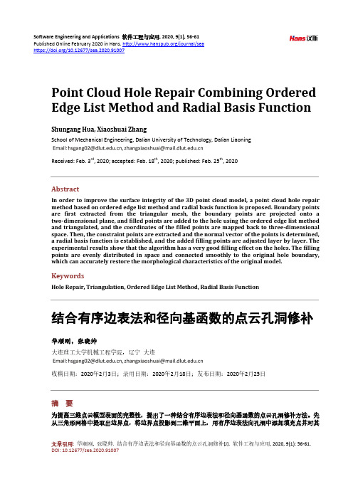
ISSN1004⁃9037，CODEN SCYCE4Journal of Data Acquisition and Processing Vol.34，No.3，May2019，pp.491-499 DOI：10.16337/j.1004⁃9037.2019.03.012Ⓒ2019by Journal of Data Acquisition and Processinghttp：//E⁃mail：sjcj@ Tel/Fax：+86⁃025⁃84892742自适应步长的Alpha‑shape表面重建算法李世林李红军（北京林业大学理学院，北京，100083）摘要：三维物体表面重建在现代临床医学、场景建模和林业测量等方面有着重要应用价值。

为了更好地理解三维物体表面形状，本文先介绍了三维空间离散点集的Alpha形状的相关概念。

在分析表面重建的Alpha⁃shape算法的基础上，本文提出一种自适应步长的Alpha⁃shape算法。

通过kd⁃tree和k近邻平均距离来动态更新α值，使得算法在处理点集密度较大的区域时也能以较少的遍历次数进行表面重建，从而改善了重建效果并提高了算法运行效率。

大量随机数据和现实三维采样数据的实验结果表明，本文提出的改进算法与原始算法相比，能大幅度地提高运行效率。

关键词：表面重建；Alpha形状；k近邻平均距离；Alpha⁃shape算法中图分类号：TP391,TP311文献标志码：ASurface Reconstruction Algorithm Using Self‑adaptive Step Alpha‑shapeLi Shilin,Li Hongjun(College of Science,Beijing Forestry University,Beijing,100083,China)Abstract：3D object surface reconstruction has important applications in modern clinical medicine，scene modeling and forestry survey and so on.In order to better understand the reconstruction of3D object surface，this paper first introduces the concept of the Alpha shape of the3D discrete point set.Based on the analysis of surface reconstruction algorithm using self⁃adaptive step Alpha⁃shape is proposed.The value of Alpha is updated dynamically using the kd⁃tree structure and the average distance of k⁃nearest neighbors，so that the algorithm can reconstruct the surface with less number of times when the density of the point set is larger.Thus，the reconstruction effect is improved and the operation efficiency of the algorithm is improved.The experimental results with a large number of random data and realistic3D scanning data show that the proposed algorithm can greatly improve the efficiency compared with the original algorithm. Key words:surface reconstruction;Alpha shape;average distance of k⁃nearest neighbors;Alpha⁃shape algorithm引言三维物体表面重建是获取三维空间信息建立该物体的三维模型，在3D城市、3D游戏等场景建模有着重要应用[1]；在林业信息化测量中，利用重建的树冠形状，准确求解树冠体积、表面积和占地面积等信基金项目：国家自然科学基金（61372190）资助项目。

INTERSECTION TRAFFIC CHANNELIZA TION MODE BASED ONHARMONIOUS TRAFFICAbstract：Based on the characteristics and aims of harmonious traffic，this paper analyzes the characteristics of intersection traffic channelization. Considering the serious traffic conflict resulted from mixed traffic of ChengDu.This paper observes the basic principles which guarantee traffic safety and furthest improve intersection capacity, emphasizes the safety and convenience for pedestrian and bicyclist crossing, combines the traffic channelization design with urban landscape design to emphasize the environmental benefits of intersection. This paper discussed mainly the theory and methods of traffic channelization including the organization of temporal and spatial separation of motor and non-motor, the traffic island design and so on and finally put forward the original intersection traffic channelization mode , which is safe, efficient, convenient and environmental and successfully applied to the project of Yu Daiqiao intersection reconstruction.Key words:Traffic Channelization, Harmonious Traffic, Intersection1 IntroductionWith regard to the mixed traffic characteristics in China, like Chengdu which has a high density of population, a large proportion of bicycling travel and serious conflicts between motor and non-motor, a scientific and effective traffic channelization model is urgently demanded, which can enhance the safety and capacity of intersections and the convenience of pedestrian and bicyclist behavior, and combine the traffic channelization with the landscape design to optimize the comprehensive benefits and construct the harmonious traffic.2 Intersection Traffic Channelization Characteristics Based on Harmonious TrafficIn<Chengdu Urban Transport Development White Paper>(2005), we put forward that the strategic concept is to construct harmonious traffic, of which two basic characteristics are humanism and environmentalism and three critical objectives are safety, convenience and environmentalism are as follows.1) Service pattern which fully protects the weak transportation communityIn view of released traffic energy risk degree of different traffic modes, thepedestrians and bicyclists are classified as weak transportation community and the service level gradually increases according to the rank of private car,public transportation, bicyclist and pedestrian respectively.2) SafetyWith the aid of traffic island and legible traffic signs, the distinct distinction of temporal and spatial rights among pedestrians, bicyclists and motors can be achieved to enhance traffic safety.3) People orientedThe design of traffic islands and non-barrier facility and so on should meet the demand of human behavior, and pay attention to the demand of disable group.4) The Optimization of capacityIt is effective to optimize intersection capacity by reducing conflicting area, advancing the stop line, reasonably arranging the entry and exit approaches.5) Environment friendlyTraffic channelization should be connected with landscape design and the humanity design to improve the environmental benefit of intersections.3 A Case Study of Chengdu3.1 Analysis on intersection and its traffic demand characteristics of ChengduWalking and bicycling accounts for a large proportion in travel behavior, which respectively is 27.2% and 36.0%. The non-motor traffic volume on Arterial road reaches to 5000 bicycles each peak hour and the acreage in most arterial intersections is above 2500 m². Though the commodious intersection space resources accommodate the interchanging demand between pedestrians and bicycles or motors, the lack of reasonable traffic channelization, the low utility of space resources,and the serious conflict greatly restrict the intersection capacity(table.1).Fig.1 Temporal and spatial separation of motor and non-motorized traffic3.2 Temporal and spatial separation of motor and non-motorAccording to the commodious space resources and the serious traffic conflict, temporal and spatial separation of motor and non-motor should be conducted at intersections to classify the road rights of pedestrians, bicycles and motors in time and space. With regard to the spatial road rights the motors, pedestrians and bicycles should be restricted to travel in different areas and bicycles travel anticlockwise while the pedestrians get a bidirectional crossing (fig.1).3.3 Placement of Entry and Exit lanesThe number of entry lanes should more than the exit. Methods that can be adopted to add entry lanes include offsetting median pavement marking, enlarging the entry approaches or removing the median closure while considering matching the number of entry lanes with road capacity. The suggested proportion of the number of entry lanes to that of lanes on road in signal direction is 1:1~2:1 (fig.2).Fig.2 methods to add entry lanesTable 2 Relationship between lanes on road (one way) and entry lanes at3.4 Traffic Island Design1)the location of traffic islandThe location of traffic island should reasonably guide motor and non-motor traffic flow, reduce the severity of conflict, ensure security and enhance the capacity. The location of island is related to the placement of advanced right-turn lane. When the angle of two crossing roads is less than 75°and there is enough space resources for pedestrian refuge, advanced right-turn lane should be adopted, or else not(fig.3, fig.4,tab.3).Fig3 Location of traffic island Fig4 location of traffic island (without advanced right-turn lane) (with advanced right-turn lane)Tab.3 Parameters related to the location of islandfootnote:R’—the minimal turning radii L’—vehicle width R—turning radii of advanced right turn lane L—vehicle length2) The refuge area of traffic islandThe refuge area of traffic island should be no less than 5.0m2. Pavement markings can be adopted while the area is too limited. The area on safety island should be large enough to accommodate the minimal need of pedestrians and the bicyclists waiting in red time.Model lists as follow:A=(Q p·T p·A p+Q b·T b·A b)S a·S l/3600 (1) In the equation:A—The refuge area of traffic island (m²);Q p，Q b—the arrival rate of pedestrians and bicyclists (person/hour,bicycles/hour);T p，T b—the maximal red time that the pedestrian and bicyclist have waited for (second);A p，A b—the static refuge area for one person and one bicyclist. They are respectively0.6 m² and 1.6 m²;S a—safety coefficient 1.3;S l—the coefficient of service level,0.85—congestion,1—relative congestion ,2—general,3—relative comfort,5—comfort.3）traffic island designThe contour of traffic island is the combination of beeline and circular curve. The refuge area should be set inside traffic island for crossing pedestrians and bicyclists. The end of traffic island should be observable and smooth enough to direct vehicles. Considering the demand on comfort and convenience for pedestrian and bicyclist entrancing and exiting traffic island：the refuge area should higher 3-5cm than the ground, with a 1:10 conjunctive grade. Blind way should be set on the refuge area and connected with pavement (fig.5, tab.4).Fig.5 Traffic island design4) Landscape design of traffic islandThe triangular area on traffic island can be utilized to design urban greening and landscape, and the background and pattern design of refuge area can be connected with the local historical culture.4 Traffic Channelization Design of the Yu Daiqiao Roundabout Flyover4.1 Traffic Channelization DesignThe Yu Daiqiao intersection is located in the Luo Mashi CBD of Chengdu. Before reconstruction the roundabout model restricted the capacity, travelingconditions under flyover is bad and the conflict between bicyclists and pedestrians isserious. The one-way traffic control in western and northern entry approaches reduces the accessibility of the road and results in excess concentration of traffic flow. The level of service of the intersection is difficult to accommodate the demand on safety, efficiency, convenience and environmentalism. Based on the traffic demand characteristic, the channeling measures mainly include (tab.5):Before After4.2 Evaluation on traffic channelization effectA quantitative evaluation is conducted by combining the theoretical calculation and traffic micro-simulation (table.6). Besides the safety and convenience of pedestriancrossing is largely enhanced, the landscaping benefit at intersection is promoted, and the road accessibility is improved through optimizing the organization of traffic flow while the business turnover around the area increases by 12 percents.footnote:“Before, After” respectively represents before and after traffic channelization.5. ConclusionConsidering the coexisting situations of serious conflicts between motors and bicyclists, the commodious space resources and low utility at intersections, the traffic channelization mode based on the harmonious traffic, which is characterized as safety, effectively, convenience and environmentalism, connects the intersection traffic channelization and urban landscape design by separating motors andnon-motors in time and space and setting traffic islands, guaranteeing the safety and convenience of pedestrian and bicyclist crossing and the efficient travel inside intersection as well as beautifying urban environment. This mode has been successfully applied to the reconstruction project of Yu Daiqiao intersection and received obvious social benefits.基于和谐交通的交叉口交通渠模式摘要基于和谐交通的特征和目的，本文分析交叉口交通渠化的特点。

Proceedings of the 2007 Industrial Engineering Research ConferenceG. Bayraksan, W. Lin, Y. Son, and R. Wysk, eds.Periodic Loci Surface Reconstruction in Nano Material DesignYan WangDepartment of Industrial Engineering and Management SystemsUniversity of Central FloridaOrlando, FL 32816, USAAbstractRecently we proposed a periodic surface (PS) model for computer aided nano design (CAND). This implicit surface model allows for parametric model construction at atomic, molecular, and meso scales. In this paper, loci surface reconstruction is studied based on a generalized PS model. An incremental searching algorithm is developed to reconstruct PS models from crystals. Two metrics to measure the quality of reconstructed loci surfaces are proposed and an optimization method is developed to avoid overfitting.KeywordsPeriodic surface, implicit surface, computer-aided nano-design, reverse engineering1. IntroductionComputer-aided nano-design (CAND) is an extension of computer based engineering design traditionally at bulk scales to nano scales. Enabling efficient structural description is one of the key research issues in CAND. Traditional boundary-based parametric solid modeling methods do not construct nano-scale geometries efficiently due to some special characteristics at the low levels. For example, the boundaries of atoms and molecules are vague and indistinguishable. Volume packing of atoms is the major theme in crystal or protein structures, which have much more complex topology than macro-scale structures. Non-deterministic geometries and topologies are the manifestations of thermodynamic and kinetic properties at the molecular scale.With the observation that hyperbolic surfaces exist in nature ubiquitously and periodic features are common in condensed materials, we recently proposed an implicit surface modeling approach, periodic surface (PS) model [1, 2], to represent the geometric structures in nano scales. This model enables rapid construction of crystal and molecular models. At the molecular scale, periodicity of the model allows thousands of particles to be built efficiently. At the meso scale, inherent porosity of the model is able to characterize morphologies of polymer and macromolecules. Some seemingly complex shapes are easy to build with the PS model.Periodic surfaces are either loci (in which discrete particles are embedded) or foci (by which discrete particles are enclosed). In this paper, we study loci surface reconstruction for reverse engineering purpose. The PS model is generalized with geometric and polynomial description. An incremental searching algorithm is developed to reconstruct loci surfaces from crystals. In the rest of the paper, Section 2 reviews related work. Section 3 describes the generalized PS model. Section 4 presents an incremental searching algorithm, illustrates with several examples, and proposes evaluation metrics for the quality of reconstructed surfaces.2. Background and Related Work2.1 Molecular Surface ModelingTo visualize 3D molecular structures, there has been some research work on molecular surface modeling [3]. Lee and Richards [4] first introduced solvent-accessible surface, the locus of a probe rolling over Van der Waals surface, to represent boundary of molecules. Connolly [5] presented an analytical method to calculate the surface. Recently, Bajaj et al. [6] represent solvent accessible surface by NURBS (non-uniform rational B-spline). Carson [7] represents molecular surface with B-spline wavelet. These research efforts concentrate on boundary representation of molecules mainly for visualization, while model construction itself is not considered.2.2 Periodic SurfaceWe recently proposed a periodic surface (PS) model to represent nano-scale geometries. It has the implicit formC p Ak k k k k =+⋅=∑]2cos[)(λπψ)(r h r (1)where r is the location vector in Euclidean space 3E , k h is the k th lattice vector in reciprocal space, k A is the magnitude factor, k λ is the wavelength of periods, k p is the phase shift, and C is a constant. Specific periodicstructures can be modeled based on this generic form. The periodic surface model can approximate triply periodic minimal surfaces (TPMSs) very well, which have been reported from atomic to meso scales. Compared to the parametric TPMS representation known as Weierstrass formula, the PS model has a much simpler form.Figure 1 lists some examples of PS models, including TPMS structures, such as P-, D-, G-, and I-WP cubic morphologies which are frequently referred to in chemistry literature. Besides the cubic phase, other mesophase Mesh MembraneFigure 1: Periodic surface models of cubic phase and mesophase structures 3. Generalized Periodic Surface ModelIn this paper, periodic surface model is generalized with geometric and polynomial descriptions. This generalization allows us to interpret control parameters geometrically and manipulate surfaces interactively. A periodic surface is defined as()0)(2cos )(11=⋅=∑∑==L l M m T m l lm r p r πκµψ (2) where l κ is the scale parameter , T m m m m m c b a ],,,[θ=p is a basis vector , such as one of{}⎪⎪⎪⎭⎪⎪⎪⎬⎫⎪⎪⎪⎩⎪⎪⎪⎨⎧⎥⎥⎥⎥⎥⎦⎤⎢⎢⎢⎢⎢⎣⎡−⎥⎥⎥⎥⎥⎦⎤⎢⎢⎢⎢⎢⎣⎡−⎥⎥⎥⎥⎥⎦⎤⎢⎢⎢⎢⎢⎣⎡−⎥⎥⎥⎥⎥⎦⎤⎢⎢⎢⎢⎢⎣⎡−⎥⎥⎥⎥⎥⎦⎤⎢⎢⎢⎢⎢⎣⎡−⎥⎥⎥⎥⎥⎦⎤⎢⎢⎢⎢⎢⎣⎡−⎥⎥⎥⎥⎥⎦⎤⎢⎢⎢⎢⎢⎣⎡⎥⎥⎥⎥⎥⎦⎤⎢⎢⎢⎢⎢⎣⎡⎥⎥⎥⎥⎥⎦⎤⎢⎢⎢⎢⎢⎣⎡⎥⎥⎥⎥⎥⎦⎤⎢⎢⎢⎢⎢⎣⎡⎥⎥⎥⎥⎥⎦⎤⎢⎢⎢⎢⎢⎣⎡⎥⎥⎥⎥⎥⎦⎤⎢⎢⎢⎢⎢⎣⎡⎥⎥⎥⎥⎥⎦⎤⎢⎢⎢⎢⎢⎣⎡⎥⎥⎥⎥⎥⎦⎤⎢⎢⎢⎢⎢⎣⎡=……11111111111111101101101111111110110110111100101010011000,,,,,,,,,,,,,,131211109876543210e e e e e e e e e e e e e e (3)which represents a basis plane in the projective 3-space 3P , T w z y x ],,,[=r is the location vector with homogeneous coordinates, and lm µis the periodic moment . We assume 1=w throughout this paper if not explicitly specified. It is also assumed that the scale parameters are natural numbers (N ∈l κ).If mapped to a density space T M s s ],,[1…=s where ))(2cos(r p ⋅=T m m s π, )(s ψcan be represented in a polynomial form, known as Chebyshev polynomial,)1()()(11≤=∑∑==m L l M m m lm s s T l κµψs (4)where ()s s T 1cos cos )(−=κκ. In a Hilbert space, the basis functions κT ’s are orthogonal with respect to density in the normalized domain, with the inner product defined as⎪⎪⎩⎪⎪⎨⎧≠===≠=−=∫−)0(2/)0()(0)()(11:,112j i j i j i ds s T s s T T j i j i ππ (5) where both i and j are natural integers (N ∈j i ,). Orthonormal bases are particularly helpful in surface reconstruction. The periodic moments are determined by the projection)0()()(112,,112≠−==∫−j ds s T s f s T T T f j j j jj πµ (6)Lemma 1. If a periodic surface )(r ψ is scaled up or down to )('r ψ, and there are no common basis vectors at the same scales between the two, then )(r ψ is orthogonal to )('r ψ.4. Loci Surface Reconstruction3D crystal or protein structures are usually inferred by using experimental techniques such as X-ray crystallography and archived in structure databases. Given actual crystal structures, loci surfaces can be reconstructed. This reverse engineering process is valuable in nano material design. It can be widely applied in material re-engineering and re-design, comparison and analysis of unknown structures, and improving interoperability of different models. In general, the loci surface reconstruction process is to find a periodic surface )(r ψ to approximate the original but unknown surface )(r f , assuming there always exists a continuous surface )(r f that passes through a finite number of discrete locations in 3E . Determining the periodic moments from the given locations is the main theme.4.1 Incremental Searching AlgorithmIn the case of sparse location data, spectral analysis is helpful to derive periodic moments. Given N known positions ),,1(3N n n …=∈P r through which a loci surface passes, loci surface reconstruction is to find a 0)(=r ψ such that the sum of Lp norms is minimized in∑=N n p n1)(min r ψ (7)Given a set of scale parameters ),,1(L l l …=κ and a set of basis vectors ),,1(M m m …=p , deriving the moments can be reduced to solving the linear system()()N n L l M m lm n T m l ,,10)(2cos 11…==⋅∑∑==µπκr p (8) or simply denoted as 01=××LM LM N µA(9) Solving (9) is to find the null space of A . The singular value decomposition (SVD) method can be applied. If the decomposed matrix is T LMLM k LM LM j LM N i v w u ×××=][][][A , any column of ][k v whose corresponding j w is zero yields a solution. With the consideration of experimental or numerical errors, least-square approximation is usually used in actual algorithm implementation. We select the last column of ][k v as the approximated solution.In general cases, the periodic vectors and scale parameters may be unknown, an incremental searching algorithm is developed to find moments as well as periodic vectors and scale parameters, as shown in Figure 2. We can use a general set of periodic vectors such as the one in (3) and incrementally reduce the scales (i.e., increase scale parameters). The searching process continues until the maximum approximation error )(max n nr ψ is less than a threshold.In the Hilbert space, the orthogonality of periodic basis functions allows for concise representation in reconstruction. In the incremental searching, the newly created small scale information in iteration t is an approximation of the difference between the original surface )(r f and the previously constructed surface )()1(r −t ψ in iteration 1−t .Input : location vectors ),,1(N n n …=rOutput : periodic moments }{lm µ, scale parameters }{l κ, and periodic vectors }{m p1. Normalize coordinates n r if necessary (e.g. limit them within the range of [0,1]);2. Set an error threshold ε;3. Initialize periodic vectors }{}{0)0(e p =m , initialize scale parameter }1{}{)0(=l κ, t =1;4. Update the periodic vectors },,{}{}{1)1()(M t m t m e e p p …∪=−, update the scale parameters with anew scale t s so that }{}{}{)1()(t t l t l s ∪=−κκ;5. Decompose matrix ()[]T n T m l t UWV r p A =⋅=)(2cos )(πκ and find )(t µ as the last column of V ; 6. If ε<⋅)()(max t t nµA , stop; otherwise, t =t +1, go to Step 4 and repeat.Figure 2: Incremental searching algorithm for loci surface reconstructionLemma 2. If the original surface )(r f is dtimes continuously differentiable, the convergence rate of the incremental searching algorithm is )(d O −κ where κ is the scale parameter.4.2 ExamplesAs the first example, we reconstruct the periodic surface model of a Faujasite crystal. As shown in Figure 3-a, each vertex in the polygon model represents a Si atom of the crystal. Within a periodic unit, we apply the incremental searching algorithm to it. With different stopping criteria, we have two surfaces with 14 and 15 vectors, as shown in Figure 3-b and Figure 3-c respectively. The reconstructed surfaces are listed in Table 1.(a) Faujasite crystal (b) Reconstructed surfacedim.=14, max_error=0.6691 (c) Reconstructed surface dim.=15, max_error= 1.686e-15 Figure 3: Loci surfaces of a Faujasite crystal with 232 atomsTable 1: PS models of the Faujasite crystal in Figure 3 with different dimensionsDimension PS model14 ))(2cos(414070))(2cos(414070))(2cos(414070))(2cos(440820))(2cos(0119920))(2cos(0119920))(2cos(0119920))(2cos(00394820))(2cos(00394820))(2cos(00394820)2cos(00859260)2cos(00859260)2cos(0085926053909.0z y x .x z y .z y x .z y x .z y .x z .y x .z y .z x .y x .z .y .x .−++−+++−+++−−−−−−−+−+−+−−−−−πππππππππππππ15 ))(4cos(0720760))(4cos(0720760))(4cos(0720760))(4cos(0720760))(4cos(103620))(4cos(103620))(4cos(103620))(4cos(103620))(4cos(103620))(4cos(103620))(2cos(402460))(2cos(402460))(2cos(402460))(2cos(402460516620z y x .x z y .z y x .z y x .z y .x z .y x .z y .z x .y x .z y x .x z y .z y x .z y x ..−++−+++−++++−+−+−++−+−+−−+−−+−+−−+++ππππππππππππππThe second example includes surface models of a synthetic Zeolite crystal, as in Figure 4-a. Each vertex represents an O atom. Three surfaces with different numbers of vectors thus different resolutions are shown in Figure 4-b, -c, and -d. The PS models are listed in Table 2.(a) Zeolite crystal (b) Reconstructed surfacedim.=14, max_error=0.2515 (c) Reconstructed surface dim.=24, max_error=0.0092(d) Reconstructed surface dim.=33, max_error=3.059e-15 Figure 4: Loci surfaces of a synthetic Zeolite crystal with 312 atomsTable 2: PS models of the synthetic Zeolite crystal in Figure 4 with different dimensions DimensionPS model 14 ))(2cos(432910))(2cos(432910))(2cos(432910))(2cos(432910))(2cos(001388.0))(2cos(001388.0))(2cos(001388.0))(2cos(001388.0))(2cos(001388.0))(2cos(001388.0)2cos(288870)2cos(288870)2cos(2888700037436.0z y x .x z y .z y x .z y x .z y x z y x z y z x y x z .y .x .−+−−+−+−−++−−+−+−+++++++−−−−πππππππππππππ24 ))(4cos(15927.0))(4cos(15927.0))(4cos(15927.0))(4cos(15927.0))(4cos(24617.0))(4cos(24617.0))(4cos(24617.0))(4cos(24617.0))(4cos(24617.0))(4cos(24617.0)4cos(32147.0)4cos(32147.0)4cos(32147.0))(2cos(000718640))(2cos(000718640))(2cos(000718640))(2cos(000718640))(2cos(18191.0))(2cos(18191.0))(2cos(18191.0))(2cos(18191.0))(2cos(18191.0))(2cos(18191.016232.0z y x x z y z y x z y x z y x z y x z y z x y x z y x z y x .x z y .z y x .z y x .z y x z y x z y z x y x −+−−+−+−−++−−−−−−−+−+−+−−−−−++−+++−++++−+−+−+++++++−πππππππππππππππππππππππ33 ))(8cos(0091814.0))(8cos(0091814.0))(8cos(0091814.0))(8cos(0091814.0))(8cos(081757.0))(8cos(081757.0))(8cos(081757.0))(8cos(081757.0))(8cos(081757.0))(8cos(081757.0)8cos(11405.0)8cos(11405.0)8cos(11405.0))(4cos(020038.0))(4cos(020038.0))(4cos(020038.0))(4cos(020038.0))(4cos(098288.0))(4cos(098288.0))(4cos(098288.0))(4cos(098288.0))(4cos(098288.0))(4cos(098288.0)4cos(086043.0)4cos(086043.0)4cos(086043.0))(2cos(37384.0))(2cos(37384.0))(2cos(37384.0))(2cos(37384.0))(2cos(37384.0))(2cos(37384.001531.0z y x x z y z y x z y x z y x z y x z y z x y x z y x z y x x z y z y x z y x z y x z y x z y z x y x z y x z y x z y x z y z x y x −++−+++−++++−−−−−−+−+−+−−−−−+−−+−+−−++−−−−−−−+−+−+−−−−−+−+−+++++++ππππππππππππππππππππππππππππππππ4.3 Quality of SurfaceThe maximum approximation error used in the incremental searching algorithm is not the only metric to measure the quality of reconstructed surfaces. It should be recognized that the maximum approximation error may cause overfitting during the least square error reconstruction. Thus, another proposed metric to measure the quality of loci surfaces is porosity , which is defined as())(/)(:32P D D D ⊆=∫∫∫∫∫∫∈∈r r r r r d d M ψψφ (11) where )(max r r ψψD ∈∀=M . The porosities of reconstructed surfaces in Figure 3 and Figure 4 are listed in Table 3. Givena fixed number of known positions that surfaces pass through, there are an infinite number of surfaces can be reconstructed. Intuitively, the surfaces with unnecessarily high surface areas have low porosities, which should be avoided.Table 3: Metrics comparison of different PS surfacesDimension Maximum approximation errorPorosity14 0.6691 0.2115Faujasite surface (Figure 3) 15 1.686e-15 0.122614 0.2515 0.0073824 0.0092 0.0394Zeolite surface (Figure 4) 33 3.059e-15 0.0829The quality of reconstructed surfaces depends on the selection of periodic vectors, scale parameters, and volumetric domain of periodic unit. Based on porosity, a surface optimization problem is to solve()),,1()(max ..},{},{max N n t s n n l m …=≤εψκφr p D(12)We apply (12) to optimize basis vectors ),,(m m m c b a of the PS model of Zeolite crystal in Figure 4. The result is shown in Figure 5 and Table 4. The dimension is reduced from 33 to 25 while porosity is increased to 0.1140 with a similar maximum approximation error.Figure 5: Optimized Zeolite surfaceTable 4: Optimized PS model of the synthetic Zeolite crystal in Figure 5Optimized PS model Dimension = 25Porosity = 0.1140Max Approx. Error= 2.1417e-15 ))(8cos(1013.0))(8cos(1013.0))(8cos(1013.0))(8cos(1013.0))(8cos(1013.0))(8cos(1013.0)8cos(13904.0)8cos(13904.0)8cos(13904.0))(4cos(072615.0))(4cos(072615.0))(4cos(072615.0))(4cos(072615.0))(4cos(072615.0))(4cos(072615.0)4cos(036561.0)4cos(036561.0)4cos(036561.0))(2cos(37489.0))(2cos(37489.0))(2cos(37489.0))(2cos(37489.0))(2cos(37489.0))(2cos(37489.0038986.0z y x z y x z y z x y x z y x z y x z y x z y z x y x z y x z y x z y x z y z x y x −+−+−++++++++++−+−+−++++++++++−−−−−−+−+−+−−ππππππππππππππππππππππππ6. Concluding RemarksIn this paper, loci surface reconstruction is studied based on the generalized periodic surface model. An incremental searching algorithm is developed to reconstruct loci surfaces from crystals. To avoid overfitting, metrics of surface quality are proposed and an optimization method is developed. Future research will include reconstruction of foci surfaces.AcknowledgementThis work is supported in part by the NSF CAREER Award CMMI-0645070.References1. Wang, Y., 2006, “Geometric modeling of nano structures with periodic surfaces,” Lecture Notes inComputer Science, 4077, 343-3562. Wang, Y., 2007, “Periodic surface modeling for computer aided nano design,” Computer-Aided Design,39(3), 179-1893. Connolly, M.L., 1996, “Molecular surfaces: A review, Network Science,”/Science/Compchem/index.html4. Lee, B., Richards, F.M., 1971, “The interpretation of protein structures: Estimation of static accessibility,”Journal of Molecular Biology, 55(3), 379-4005. Connolly, M.L., 1983, “Solve-accessible surfaces of proteins and nucleic acids,” Science, 221(4612), 709-7136. Bajaj, C., Pascucci, V., Shamir, A., Holt, R., Netravali, A., 2003, “Dynamic Maintenance and visualizationof molecular surfaces,” Discrete Applied Mathematics, 127(1), 23-517. Carson, M, 1996, “Wavelets and molecular structure,” Journal of Computer Aided Molecular Design, 10(4),273-283。

面部创伤的“无痕”修复【摘要】面部的外观在人的整体外貌中起到至关重要的作用，拥有一副赏心悦目的面孔有时会影响一个人的一生[1]，因此无论是以单纯改善外观的整形目的来就诊，还是以创伤后修复为目的来就诊，都是为了让自己的容貌能够变得更出众或者将外伤对容貌的损伤降到最低，对于单纯求美者来说，悦人的同时更是为了悦己，而对于面部创伤的患者，创伤后的“无痕”修复对患者日后正常生活有着至关重要的作用[2]。

【关键词】面部创伤；拉拢缝合；皮瓣修复；瘢痕预防；瘢痕综合治疗【中图分类号】R473【文献标识码】A【文章编号】2096-0867（2016）13-226-01瘢痕重在预防，早期预防比后期治疗更为重要，瘢痕前期预防较欠缺的情况下，后期再进行充分的治疗也只能起到略微减轻瘢痕增生的作用，终究无法弥补早期治疗欠缺所造成的缺憾。

创伤后6-8小时内给予及时、平整的清创缝合，术后及时换药，必要时口服抗生素预防感染，术后适时的拆线，同时结合后期局部加压，涂抹硅凝胶，点阵激光，同位素放射治疗，曲安奈德瘢痕内注射等综合疗法对瘢痕进行防治。

一、瘢痕预防瘢痕预防中最为重要的是外伤后能将组织对合平整，且术中操作要轻柔，避免造成额外的组织损伤。

对于创缘比较整齐的刀砍伤可用5-0薇荞线做皮下减张后直接用6-0丝线拉拢缝合。

其余外伤所致的创口一般情况下创缘不平整，对于两侧形成厚薄不一的创面皮下使用5-0可吸收缝线进行对合显得尤为重要，此时需在较薄的一侧进针，较厚的一侧出针，较薄的一侧进针较浅，皮下组织较少，较厚的一侧进针较深，皮下组织较多，打结后观察两侧创缘是否在同一个水平面上，以便纠正创伤造成的高低不平的外观，皮肤使用6-0无创丝线进行缝合，避免术后由于针眼及缝线压迫而形成“蜈蚣”样瘢痕影响美观。

对于挫裂伤等不平整的锯齿状创缘缝合前视周围皮肤松弛状况应用整形剪刀刷缘后再进行缝合。

缝合前可对创口方向进行适当的调整，使其于面部张力线[3]之间的夹角达到最小以减小术后切口张力，减轻局部瘢痕增生。

前庭导水管扩大合并内耳畸形的影像学分析邢庆娜;张小安;赵鑫;姚晓宾【摘要】目的:探讨前庭导水管扩大(EVA)和耳蜗发育异常、前庭耳蜗发育不良等内耳畸形间的关系.方法:回顾性分析郑州大学第三附属医院2010-2012年诊断为EVA的患者30例60耳.均行MSCT及MRI检查,评估EVA患者合并的其他内耳异常.结果:选取的60耳均患有EVA,双侧EVA 26例,单侧EVA 4例,12例女性和18例男性.平均年龄1.8岁(6月～4.2岁).45(80.4％)耳EVA同时合并有一个或多个内耳异常.30(53.6％)耳合并耳蜗发育不良,9(16.1％)耳合并前庭耳蜗发育不良.结论:小视野、薄层MSCT和磁共振内耳水成像相结合,可以准确的发现EVA通常合并的内耳发育畸形,尤以耳蜗发育不良最常见.【期刊名称】《中国临床医学影像杂志》【年(卷),期】2014(025)001【总页数】4页(P5-8)【关键词】迷路;畸形;前庭;体层摄影术,螺旋计算机;磁共振成像【作者】邢庆娜;张小安;赵鑫;姚晓宾【作者单位】郑州大学第三附属医院放射科,河南郑州450052;郑州大学第三附属医院放射科,河南郑州450052;郑州大学第三附属医院放射科,河南郑州450052;河南省肿瘤医院检验科,河南郑州450008【正文语种】中文【中图分类】R764.73;R445.2;R814.42前庭导水管扩大（EVA）最早由Carolo Mondini在1791年解剖一个先天性耳聋的孩子颞骨时发现。

前庭导水管是在颞骨岩部内骨性通道，容纳了淋巴管和淋巴囊以及静脉前庭导水管。

EVA可能是由于胚胎发育过程中淋巴管和淋巴囊异常的扩大和扩张所致。

EVA已经被认为是最常见的内耳畸形，伴有感音神经性听力损失。

EVA往往合并其他内耳畸形，如与耳蜗发育不良存在一定的关联，这可能是造成听力损失的真正原因。

随着医学影像学的发展，能够更容易地识别以前还没有被确定的其他内耳异常。

第52卷第12期表面技术2023年12月SURFACE TECHNOLOGY·197·化学刻蚀-阳极氧化复合制备钛合金超疏水表面试验研究马宁，张鑫宇，孙岩，龙芳宇，孙凯伦（沈阳航空航天大学 机电工程学院，沈阳 110136）摘要：目的提高TC4钛合金超疏水表面的疏水性、耐腐蚀性与力学性能。

方法首先选择化学刻蚀法对TC4钛合金进行处理制备出微米级结构，再采用阳极氧化法制备出纳米级结构，最终在试样表面制备出了具有微纳分级结构的超疏水表面。

通过观察微观结构表面、Tafel测试、线性磨损试验、抗冲击性测试以及防冰性能测试，分别对H2O2刻蚀、强酸刻蚀、阳极氧化、H2O2刻蚀-阳极氧化和强酸刻蚀-阳极氧化制备的超疏水表面进行性能对比。

结果使用双氧水-碳酸氢钠混合溶液制备出的超疏水表面接触角为156.4°，滚动角为2.7°；硫酸-盐酸混合溶液制备出的超疏水表面接触角为153.1°，滚动角为7.6°；阳极氧化法制备的超疏水表面接触角为156.3°，滚动角为4.2°；双氧水-碳酸氢钠混合溶液刻蚀并阳极氧化处理后，表面接触角为157.6°，使用硫酸-盐酸混合溶液刻蚀并阳极氧化处理后，表面接触角为155.9°，二者滚动角均小于2°。

复合方法制备的表面疏水性能优于单一方法制备的超疏水表面。

超疏水试样的OCP都高于TC4钛合金，经过强酸刻蚀和阳极氧化处理后的超疏水试样，其OCP正移到0.08 V，J corr降低了1个数量级，R p增大了1个数量级，耐腐蚀性能明显提高。

复合方法制备的超疏水表面在经过多次线性磨损以及经历200 g落沙冲击后，表面接触角仍能保持150°以上，滚动角为10°左右，仍保持了超疏水性能。

结论采用复合方法制备的具有微纳分级结构的超疏水表面相较于单一结构的超疏水表面具有更好的疏水性、耐腐蚀性、耐磨损性和抗冲击性。

银川海派英语【SAT2化学】备考知识点之三种状态Liquids Solids and Phase Changes 液体，固体和状态变化Liquids(液体) Importance of Intermolecular Interaction(分子间相互作用的重要性)Kinetics of Liquids(液体动力学)Viscosity(粘性)Surface Tension(表面张力)Capillary Action(毛细作用)Phase Equilibrium(平衡状态)Boiling Point(沸点)Critical Temperature and Pressure(临界温度和临界压力)Solids(固体) Phase Diagrams(状态图表)Water(水)History of Water(水的历史)Purification of Water(水净化)Composition of Water(水的构成)Properties and Uses of Water(水的性质和使用)W ater’s Reactions with Anhydrides(水和碱性氧化物的反应)Polarity and Hydrogen Bonding(极性和氢键)Solubility(可溶性)General Rules of Solubility(可溶性的基本原则)Factors That Affect Rate of Solubility(影响溶解率的因素)Summary of Types of Solutes and Relationships of Type to Solubility(溶液类型和类型之间关系的总结)Water Solutions(水处理)Continuum of Water Mixtures(水混合溶剂)exxxxxpressions of Concentration(浓度的表达)Dilution(稀释)Colligative Properties of Solutions(溶液的依数性)Crystallization(结晶化)以上就是关于SAT2化学知识点中三种状态的总结，都是一些比较琐碎的点。