风险管理与金融机构第二版课后习题答案 (修复的)(1)概述

风险管理与金融机构第二版课后习题答案第八章8.1VaR是指在一定的知心水平下损失不能超过的数量；预期亏损是在损失超过VaR的条件下损失的期望值，预期亏损永远满足次可加性（风险分散总会带来收益）条件。

8.2一个风险度量可以被理解为损失分布的分位数的某种加权平均。

VaR对于第某个分位数设定了100%的权重，而对于其它分位数设定了0权重，预期亏损对于高于某%的分位数的所有分位数设定了相同比重，而对于低于某%的分位数的分位数设定了0比重。

我们可以对分布中的其它分位数设定不同的比重，并以此定义出所谓的光谱型风险度量。

当光谱型风险度量对于第q个分位数的权重为q的非递减函数时，这一光谱型风险度量一定满足一致性条件。

8.3有5%的机会你会在今后一个月损失6000美元或更多。

8.4在一个不好的月份你的预期亏损为60000美元，不好的月份食指最坏的5%的月份8.5(1)由于99.1%的可能触发损失为100万美元，故在99%的置信水平下，任意一项损失的VaR为100万美元。

（2）选定99%的置信水平时，在1%的尾部分布中，有0.9%的概率损失1000万美元，0.1%的概率损失100万美元，因此，任一项投资的预期亏损是0.1%1%1000.9%1%1000910万美元（3）将两项投资迭加在一起所产生的投资组合中有0.0090.009=0.000081的概率损失为2000万美元，有0.9910.991=0.982081的概率损失为200万美元，有20.0090.991=0.017838的概率损失为1100万美元，由于99%=98.2081%+0.7919%，因此将两项投资迭加在一起所产生的投资组合对应于99%的置信水平的VaR是1100万美元。

（4）选定99%的置信水平时，在1%的尾部分布中,有0.0081%的概率损失2000万美元，有0.9919%的概率损失1100万美元，因此两项投资迭加在一起所产生的投资组合对应于99%的置信水平的预期亏损是0.0000810.0120000.0099190.0111001107万美元（5）由于11001002=200，因此VaR不满足次可加性条件，11079102=1820，因此预期亏损满足次可加性条件。

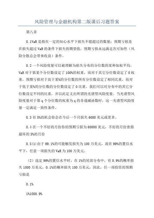
1.15假定某一投资预期回报为8%，标准差为14%；另一投资预期回报为12%，标准差为20%。

两项投资相关系数为0.3，构造风险回报组合情形。

w 1 w 2 μP σP 0.01.0 12% 20% 0.20.8 11.2% 17.05% 0.40.6 10.4% 14.69% 0.60.4 9.6% 13.22% 0.80.2 8.8% 12.97% 1.0 0.08.0% 14.00%1.166市场的预期回报为12%，无风险利率为7%，市场回报标准差为15%。

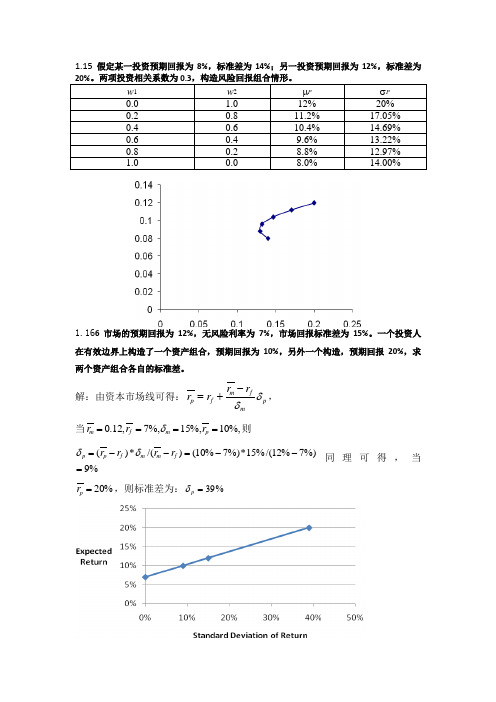
一个投资人在有效边界上构造了一个资产组合，预期回报为10%，另外一个构造，预期回报20%，求两个资产组合各自的标准差。

解：由资本市场线可得：p m fm f p r r r r δδ-+=，当%,10%,15%,7,12.0====p m f m r r r δ则%9%)7%12/(%15*%)7%10()/(*)(=--=--=f m m f p p r r r r δδ同理可得，当%20=p r ，则标准差为：%39=p δ1.17一家银行在下一年度的盈利服从正太分布，其期望值及标准差分别为资产的0.8%及2%.股权资本为正，资金持有率为多少。

在99% 99.9%的置信度下，为使年终时股权资本为正，银行的资本金持有率（分母资产）分别应为多少（1）设 在99%置信度下股权资本为正的当前资本金持有率为A ，银行在下一年的盈利占资产的比例为X ，由于盈利服从正态分布，因此银行在99%的置信度下股权资本为正的当前资本金持有率的概率为：()P X A >-，由此可得0.8%0.8%()1()1()()99%2%2%A A P X A P X A N N --+>-=-<-=-==查表得0.8%2%A +=2.33，解得A=3.85%，即在99％置信度下股权资本为正的当前资本金持有率为3.85%。

（2）设 在99.9%置信度下股权资本为正的当前资本金持有率为B ，银行在下一年的盈利占资产的比例为Y ，由于盈利服从正态分布，因此银行在99.9%的置信度下股权资本为正的当前资本金持有率的概率为：()P Y B >-，由此可得0.8%0.8%()1()1()()99.9%2%2%B B P Y B P Y B N N --+>-=-<-=-==查表得0.8%2%B +=3.10，解得B=5.38% 即在99.9％置信度下股权资本为正的当前资本金持有率为5.38%。

1.15假定某一投资预期回报为8%，标准差为14%；另一投资预期回报为12%，标准差为20%。

两项投资相关系数为0.3，构造风险回报组合情形。

1.16投资人在有效边界上构造了一个资产组合，预期回报为10%，另外一个构造，预期回报20%，求两个资产组合各自的标准差。

解：由资本市场线可得：p m fm f p r r r r δδ-+=，当%,10%,15%,7,12.0====p m f m r r r δ则%9%)7%12/(%15*%)7%10()/(*)(=--=--=f m m f p p r r r r δδ同理可得，当%20=p r ，则标准差为：%39=p δ 1.17一家银行在下一年度的盈利服从正太分布，其期望值及标准差分别为资产的0.8%及2%.股权资本为正，资金持有率为多少。

在99% 99.9%的置信度下，为使年终时股权资本为正，银行的资本金持有率（分母资产）分别应为多少（1）设 在99%置信度下股权资本为正的当前资本金持有率为A ，银行在下一年的盈利占资产的比例为X ，由于盈利服从正态分布，因此银行在99%的置信度下股权资本为正的当前资本金持有率的概率为：()P X A >-，由此可得0.8%0.8%()1()1()()99%2%2%A A P X A P X A N N --+>-=-<-=-==查表得0.8%2%A +=2.33，解得A=3.85%，即在99％置信度下股权资本为正的当前资本金持有率为3.85%。

（2）设 在99.9%置信度下股权资本为正的当前资本金持有率为B ，银行在下一年的盈利占资产的比例为Y ，由于盈利服从正态分布，因此银行在99.9%的置信度下股权资本为正的当前资本金持有率的概率为：()P Y B >-，由此可得0.8%0.8%()1()1()()99.9%2%2%B B P Y B P Y B N N --+>-=-<-=-==查表得0.8%2%B +=3.10，解得B=5.38% 即在99.9％置信度下股权资本为正的当前资本金持有率为5.38%。

风险管理与⾦融机构第⼆版课后习题答案（修复的）（1）概述1.15 假定某⼀投资预期回报为8%，标准差为14%；另⼀投资预期回报为12%，标准差为，市场回报标准差为15%。

⼀个投资⼈在有效边界上构造了⼀个资产组合，预期回报为10%解：由资本市场线可得：p m fm f p r r r r δδ-+=，当%,10%,15%,7,12.0====p m f m r r r δ则%9%)7%12/(%15*%)7%10()/(*)(=--=--=f m m f p p r r r r δδ同理可得，当%20=p r ，则标准差为：%39=p δ 1.17⼀家银⾏在下⼀年度的盈利服从正太分布，其期望值及标准差分别为资产的0.8%及2%.股权资本为正，资⾦持有率为多少。

（1）设在99%置信度下股权资本为正的当前资本⾦持有率为A ，银⾏在下⼀年的盈利占资产的⽐例为X ，由于盈利服从正态分布，因此银⾏在99%的置信度下股权资本为正的当前资本⾦持有率的概率为：()P X A >-，由此可得0.8%0.8%()1()1()()99%2%2%A A P X A P X A N N --+>-=-<-=-==查表得0.8%2%A +=2.33，解得A=3.86%，即在99％置信度下股权资本为正的当前资本⾦持有率为3.86%。

（2）设在99.9%置信度下股权资本为正的当前资本⾦持有率为B ，银⾏在下⼀年的盈利占资产的⽐例为Y ，由于盈利服从正态分布，因此银⾏在99.9%的置信度下股权资本为正的当前资本⾦持有率的概率为：()P Y B >-，由此可得0.8%0.8%()1()1()()99.9%2%2%B B P Y B P Y B N N --+>-=-<-=-==查表得0.8%2%B +=3.10，解得B=5.4% 即在99.9％置信度下股权资本为正的当前资本⾦持有率为5.4%。

1.18⼀个资产组合经历主动地管理某资产组合，贝塔系数0.2.去年，⽆风险利率为5%，回报-30%。

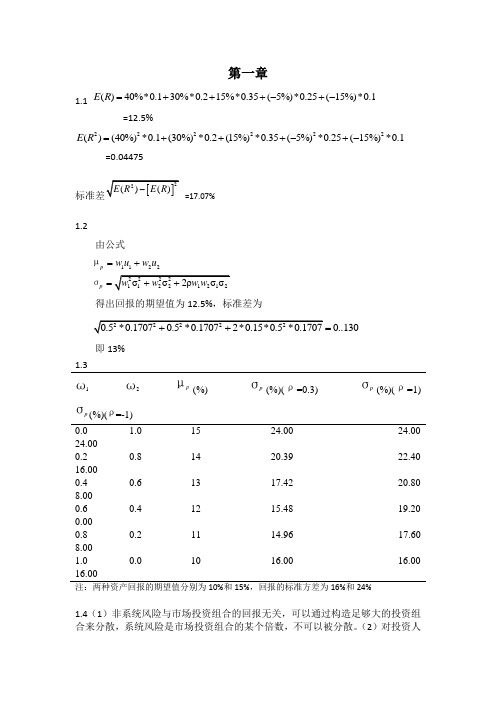
第一章1.1 ()40%*0.130%*0.215%*0.35(5%)*0.25(15%)*0.1E R =+++-+-=12.5%222222()(40%)*0.1(30%)*0.2(15%)*0.35(5%)*0.25(15%)*0.1E R =+++-+-=0.04475=17.07%1.2由公式1122p p w u w u =+=µσ得出回报的期望值为12.5%，标准差为0..130=即13%1.31ω 2ω p μ(%) p σ(%)(ρ=0.3) p σ(%)(ρ=1) pσ(%)(ρ=-1) 0.01.0 15 24.00 24.00 24.000.20.8 14 20.39 22.40 16.000.40.6 13 17.42 20.80 8.000.60.4 12 15.48 19.20 0.000.80.2 11 14.96 17.60 8.001.00.0 10 16.00 16.0016.00 注：两种资产回报的期望值分别为10%和15%，回报的标准方差为16%和24%1.4（1）非系统风险与市场投资组合的回报无关，可以通过构造足够大的投资组合来分散，系统风险是市场投资组合的某个倍数，不可以被分散。

（2）对投资人来说，系统风险更重要。

因为当持有一个大型而风险分散的投资组合时，系统风险并没有消失。

投资人应该为此风险索取补偿。

（3）这两个风险都有可能触发企业破产成本。

例如：2008年美国次贷危机引发的全球金融风暴（属于系统风险），导致全球不计其数的企业倒闭破产。

象安然倒闭这样的例子是由于安然内部管理导致的非系统风险。

1.5理论依据：大多数投资者都是风险厌恶者，他们希望在增加预期收益的同时也希望减少回报的标准差。

在有效边界的基础上引入无风险投资，从无风险投资F 向原有效边界引一条相切的直线，切点就是M ，所有投资者想要选择的相同的投资组合，此时新的有效边界是一条直线，预期回报与标准差之间是一种线性替代关系，选择M 后，投资者将风险资产与借入或借出的无风险资金进行不同比例的组合来体现他们的风险胃口。

第七章7.1大约有50亿期限超过一年的贷款是由期限小于一年的存款所支撑，换句话说，大约有50亿期限小于一年期限的负债（存款）是用于支撑期限大于一年的资产（贷款）。

当利率增长时，存款利息增加，但贷款利息却没有增加，净利息溢差收入受到压力。

7.2 S&Ls的长期固定利息的房屋贷款是由短期存款支持因此在利率迅速增长时，S&Ls会有所损失。

7.3这是利率不匹配为100亿美元，在今后3年，银行的净利息收入会每年下降1亿美元。

7.4因为如果长期利率仅仅反映了预期短期利率，我们会看到长期利率低于短期利率的情况和长期利率高于短期利率的情况一样频繁（因为投资人假设利率未来上涨和下降的概率相同），流动性偏好理论认为长期利率高于将来预期短期利率，这意味着长期利率在多数时间会高于短期利率，当市场认为利率会下跌时，长期利率低于短期利率。

7.5金融机构一般是将LIBOR互换利率曲线作为无风险利率，市场通常认为国债利率低于无风险利率，这是因为：（1）金融机构为满足一定的监管要求，必须买入一定的长期及短期国债，而这一需求造成国债收益率的降低；（2）通持与其他类似的低风险的投资相比，持有国债所需要的资本金要少；（3）在美国，对于国债的税务规定要比其他定息投资更为有利，投资政府国债而获益无需缴纳州税。

7.6久期信息用以描述了收益率小的平行移动对于债券价格的影响，交易组合价格减小的百分比等于组合久期乘以小的平行移动的数量；局限性是这一方法只适应于小的平行移动。

7.7（a）令该5年期债券的票面价格为m=100美元，根据债券价格公式，p=*e-y*ti + m* e-y*t得到，p1=86.80美元。

（b）根据债券久期公式，D=- *=-(8*e-0.11+16*e-0.22+24*e-0.33+32*e-0.44+40*e-0.55)-5*100*e-0.55=-369.42，D=-*(-369.42)=4.256得到，债券久期D=4.256。

市场的预期回报为12%，无风险利率为7%，市场回报标准差为15%。

一个投资人在有效边界上构造了一个资产组合，预期回报为10%，另外一个构造，预期回报20%，求两个资产组合各自的标准差。

解：由资本市场线可得：p m fm f p r r r r δδ-+=，当%,10%,15%,7,12.0====p m f m r r r δ则%9%)7%12/(%15*%)7%10()/(*)(=--=--=f m m f p p r r r r δδ同理可得，当%20=p r ，则标准差为：%39=p δ一家银行在下一年度的盈利服从正太分布，其期望值及标准差分别为资产的%及2%.股权资本为正，资金持有率为多少。

在99% %的置信度下，为使年终时股权资本为正，银行的资本金持有率（分母资产）分别应为多少（1）设 在99%置信度下股权资本为正的当前资本金持有率为A ，银行在下一年的盈利占资产的比例为X ，由于盈利服从正态分布，因此银行在99%的置信度下股权资本为正的当前资本金持有率的概率为：()P X A >-，由此可得0.8%0.8%()1()1()()99%2%2%A A P X A P X A N N --+>-=-<-=-==查表得0.8%2%A +=，解得A=%，即在99％置信度下股权资本为正的当前资本金持有率为%。

（2）设 在%置信度下股权资本为正的当前资本金持有率为B ，银行在下一年的盈利占资产的比例为Y ，由于盈利服从正态分布，因此银行在%的置信度下股权资本为正的当前资本金持有率的概率为：()P Y B >-，由此可得0.8%0.8%()1()1()()99.9%2%2%B B P Y B P Y B N N --+>-=-<-=-==查表得0.8%2%B +=，解得B=% 即在％置信度下股权资本为正的当前资本金持有率为%。

一个资产组合经历主动地管理某资产组合，贝塔系数.去年，无风险利率为5%，回报-30%。

风险管理与金融机构约翰第二版答案This manuscript was revised on November 28, 2020Solutions to Further ProblemsRisk Management and Financial InstitutionsSecond EditionJohn C. HullChapter 1: Introduction. The impact of investing w1 in the first investment and w2 = 1 –w1 in the second investment is shown in the table below. The range of possible risk-standard deviation of returns corresponding to an expected return of 10% is 9%. The standard deviation of returns corresponding to an expected return of 20% is 39%..(a) The bank can be 99% certain that profit will better than ×2 or –% of assets. It therefore needs equity equal to % of assets to be 99% certainthat it will have a positive equity at the year end.(b)The bank can be % certain that profit will be greater than × 2 or –% of assets. It therefore needs equity equal to % of assets to be % certain that it will have a positive equity at the year end.. When the expected return on the market is 30% the expected return on a portfolio with a beta of is+ × ( =or –2%. The actual return of –10% is worse than the expected return. The portfolio manager has achieved an alpha of –8%!Chapter 2: Banks. There is a % chance that the profit will not be worse than × =$ million. Regulators will require $ million of additional capital.. Deposit insurance makes depositors less concerned about the financial health of a bank. As a result, banks may be able to take more risk without being in danger of losing deposits. This is an example of moral hazard. (The existence of the insurance changes the behavior of the parties involved with the result that the expected payout on the insurance contract is higher.) Regulatory requirements that banks keep sufficient capital for the risks they are taking reduce their incentive to take risks. One approach (used in the US) to avoiding the moral hazard problem is to make the premiums that banks have to pay for deposit insurance dependent on an assessment of the risks they are taking.. When ranked from lowest to highest the bidders are G, D, E and F, A, C, H, and B. Individuals G, D, E, and F bid for 170, 000 shares in total. Individual A bid for a further 60,000 shares. The price paid by the investors is therefore the price bid by A ., $50). Individuals G, D, E, and F get the whole amount of the shares they bid for. Individual A gets 40,000 shares.. If it succeeds in selling all 10 million shares in a best efforts arrangement, its fee will be $2 million. If it is able to sell the sharesfor $, this will also be its profit in a firm commitment arrangement. The decision is likely to hinge on a) an estimate of the probability of selling the shares for more than $ and b) the investment banks appetite for risk. For example, if the bank is 95% certain that it will be able to sell the shares for more than $, it is likely to choose a firm commitment. But if assesses the probability of this to be only 50% or 60% it is likely to choose a best efforts arrangement.Chapter 3: Insurance Companies and Pension Funds. (Spreadsheet Provided). The unconditional probability of the man dying in years one, two, and three can be calculated from Table as follows:Year 1:Year 2: (1 × =Year 3: (1 × (1 × =The expected payouts at times , , are therefore $59,, $64,, and $68,. These have a present value of $175,. The survival probability of the man isYear 0: 1Year 1: 1 =Year 2: 1 =The present value of the premiums received per dollar of premium istherefore . The minimum premium isor $62,.(a) The losses in millions of dollars are normally distributed with mean 150 and standard deviation 50. The payout from the reinsurance contract is therefore normally distributed with mean 90 and standard deviation 30. Assuming that the reinsurance company feels it can diversify away the risk, the minimum cost of reinsurance isor $ million. (This assumes that the interest rate is compounded annually.)(b) The probability that losses will be greater than $200 million is the probability that a normally distributed variable is greater than one standard deviation above the mean. This is . The expected payoff in millions of dollars is therefore × 100= and the value of the contract isor $ million.. The value of a bond increases when interest rates fall. The value of the bond portfolio should therefore increase. However, a lower discount ratewill be used in determining the value of the pension fund liabilities. This will increase the value of the liabilities. The net effect on the pension plan is likely to be negative. This is because the interest rate decrease affects 100% of the liabilities and only 40% of the assets.. (Spreadsheet Provided) The salary of the employee makes no difference to the answer. (This is because it has the effect of scaling all numbers up or down.) If we assume the initial salary is $100,000 and that the real growth rate of 2% is annually compounded, the final salary at the end of 45 yearsis $239,. The spreadsheet is used in conjunction with Solver to show that the required contribution rate is % (employee plus employer). The value of the contribution grows to $2,420, by the end of the 45 year working life. (This assumes that the real return of % is annually compounded.) This value reduces to zero over the following 18 years under the assumptions made. This calculation confirms the point made in Section that defined benefit plans require higher contribution rates that those that exist in practice.Chapter 4: Mutual Funds and Hedge Funds. The investor pays tax on dividends of $200 and $300 in year 2009 and 2010, respectively. The investor also has to pay tax on realized capital gains by the fund. This means tax will be paid on capital gains of $500 and $300 in year 2009 and 2010, respectively The result of all this is that the basisfor the shares increases from $50 to $63. The sale at $59 in year 2011 leads to a capital loss of $4 per share or $400 in total.. The investors overall return is× × × – 1 =or % for the four years.. The overall return on the investments is the average of 5%, 1%, 10%, 15%, and 20% or %. The hedge fund fees are 2%, %, 4%, 5%, and 6%. These average %. The returns earned by the fund of funds after hedge fund fees are therefore 7%, %, 6%, 10%, and 14%. These average %. The fund of funds fee is 1% + %or % leaving % for the investor. The return earned is therefore divided as shown in the table below. This example explains why funds of funds have. The plot is shown in the chart below. If the hedge fund return is negative, the pension fund return is 2% less than the hedge fund return. If it is positive, the pension fund return is less than the hedge fund return by 2% plus 20% of the return.Chapter 5: Financial Instruments. There is a margin call when more than $1,000 is lost from the margin account. This happens when the futures price of wheat rises by more than1,000/5,000 = . There is a margin call when the futures price of wheat rises above 270 cents. An amount, $1,500, can be withdrawn from the marginaccount when the futures price of wheat falls by 1,500/5,000 = . The withdrawal can take place when the futures price falls to 220 cents.. The investment in call options entails higher risks but can lead to higher returns. If the stock price stays at $94, an investor who buys call options loses $9,400 whereas an investor who buys shares neither gains nor loses anything. If the stock price rises to $120, the investor who buys calloptions gains2000 × (120 95) 9400 = $40, 600An investor who buys shares gains100 × (120 94) = $2, 600The strategies are equally profitable if the stock price rises to a level, S, where100 × (S 94) = 2000(S 95) 9400orS = 100The option strategy is therefore more profitable if the stock price rises above $100.. Suppose S T is the price of oil at the bond’s maturity. In addition to $1000 the Standard Oil bond pays:S T< $25 : 0$40 > S T> $2 : 170 (S T 25)S T> $40: 2, 550This is the payoff from 170 call options on oil with a strike price of 25less the payoff from 170 call options on oil with a strike price of 40. The bond is therefore equivalent to a regular bond plus a long position in 170 call options on oil with a strike price of $25 plus a short position in 170 call options on oil with a strike price of $40. The investor has what is termed a bull spread on oil.. The arbitrageur could borrow money to buy 100 ounces of gold today andshort futures contracts on 100 ounces of gold for delivery in one year. This means that gold is purchased for $500 per ounce and sold for $700 per ounce. The return (40% per annum) is far greater than the 10% cost of the borrowed funds. This is such a profitable opportunity that the arbitrageur should buy as many ounces of gold as possible and short futures contracts on the same number of ounces. Unfortunately, arbitrage opportunities as profitable asthis rarely, if ever, arise in practice..(a) By entering into a three-year swap where it receives % and pays LIBORthe company earns % for three years.(b) By entering into a five-year swap where it receives % and pays LIBOR the company earns % for five years.(c) By entering into a swap where it receives % and pays LIBOR for ten years the company earns % for ten years.. The position is the same as a European call to buy the asset for K on the date..(a) When the CP rate is % and Treasury rates are 6% with semiannual compounding, the CMT% is 6% and an Excel spreadsheet can be used to showthat the price of a 30-year bond with a % coupon is about . The spread is zero and the rate paid by P&G is %.(b) When the CP rate is % and Treasury rates are 7% with semiannual compounding, the CMT% is 7% and the price of a 30-year bond with a % coupon is about . The spread is thereforemax[0, × 7/ /100]or %. The rate paid by P&G is %... The trader has to provide 60% of the price of the stock or $2,400. There is a margin call when the margin account balance as a percent of the value of the shares falls below 30%. When the share price is S the margin account balance is 2400 + 200× (S20) and the value of the position is 200×S. There is a margin call when2400 + 200 × (S20) < × 200 × Sor140 S < 1600orS <that is, when the stock price is less than $.Chapter 6: How Traders Manage Their Exposures. With the notation of the text, the increase in the value of the portfolioisThis is× 50 × 32+ 25 × 4 = 325The result should be an increase in the value of the portfolio of $325.. The price, delta, gamma, vega, theta, and rho of the option are , , , , , and . When the stock price increases to , the option price increases to . The change in the option price is = . Delta predicts a change in the option price of × = which is ver y close. When the stock price increases to , delta increases to . The size of the increase in delta is = . Gamma predicts an increase of × = which is (to three decimal places) the same. When the volatility increases from 25% to 26%, the option price increases by from to . This is consistent with the vega value of . When the time to maturity is changed from 1 to 11/365 the option price reduces by from to . This is consistent with a theta of . Finally when the interest rateincreases from 5% to 6% the value of the option increases by from to .This is consistent with a rho of .. The delta of the portfolio is1, 000 × 500 × 2,000 × ( 500 × = 450The gamma of the portfolio is1, 000 × 500 × 2,000 × 500 × = 6,000The vega of the portfolio is1, 000 × 500 × 2,000 × 500 × = 4,000(a) A long position in 4,000 traded options will give a gamma-neutral portfolio since the long position ha s a gamma of 4, 000 × = +6,000. The delta of the whole portfolio (including traded options) is then:4, 000 × 450 = 1, 950Hence, in addition to the 4,000 traded options, a short position in ￡1,950 is necessary so that the portfolio is both gamma and delta neutral.(b) A long position in 5,000 traded options will give a vega-neutralportfolio since the long position h as a vega of 5, 000 × = +4,000. The delta of the whole portfolio (including traded options) is then5, 000 × 450 = 2, 550Hence, in addition to the 5,000 traded options, a short position in ￡2,550 is necessary so that the portfolio is both vega and delta neutral.. Let w1 be the position in the first traded option and w2 be the positionin the second traded option. We require:6, 000 = +4, 000 = +The solution to these equations can easily be seen to be w1 = 3,200, w2 =2,400. The whole portfolio then has a delta of450 + 3,200 × + 2,400 × = 1,710Therefore the portfolio can be made delta, gamma and vega neutral by taking a long position in 3,200 of the first traded option, a long position in2,400 of the second traded option and a short position in ￡1,710.. (Spreadsheet Provided) Consider the first week. The portfolio consists of a short position in 100,000 options and a long position in 52,200 shares. The value of the option changes from $240,053 at the beginning of the week to $188,760 at the end of the week for a gain of $51,293.The value of the shares change from 52,200 × 49 = $2,557, 800 to 52,200 × = $2,511,864 for a loss of $45,936. The net gain is 51,293 45,936 = $5,357. The gamma and theta (per year) of the portfolio are 6, and 430,533 so that equation predicts the gain as430,533 ×1/52 + × 6, × 49)2 = 5,742. The bank has an asset-liability mismatch of $25 billion. The profit after tax is currently 12% of $2 billion or $ billion. If interest rates rise by X% the bank's before-tax loss (in billions of dollars) is 25 ××X = . After taxes this loss becomes $ × = . The bank's return on equity would be reduced to zero when = or X = . A % rise in rates would therefore reduce the return on equity to zero..(a) The duration of Portfolio A isSince this is also the duration of Portfolio B, the two portfolios do have the same duration.(b) The value of Portfolio A is2000e ×1 + 6000e ×10 = 4,When yields increase by 10 basis points its value becomes2000e ×1 + 6000e ×10 = 3,The percentage decrease in value is10095.016,477.23⨯= The value of Portfolio B is5000e × = 2,When yields increase by 10 basis points its value becomes5000 e × = 2,The percentage decrease in value isThe percentage changes in the values of the two portfolios for a 10 basis point increase in yields are therefore the same.(c) When yields increase by 5% the value of Portfolio A becomes2000e ×1 + 6000e ×10 = 3,and the value of Portfolio B becomes× = 2,The percentage reductions in the values of the two portfolios are:Portfolio A:10095.016,475.956⨯ = Portfolio B:10081.757,266.709⨯ = . For Portfolio A the convexity isFor portfolio B the convexity is or The percentage change in the twoportfolios predicted by the duration measure is the same and equal to × = or –%. However, the convexity measure predicts that the percentage change in the first portfolio will be× + × × =and that for the second portfolio it will be× = × × =Duration does not explain the difference between the percentage changes. Convexity explains part of the difference. 5% is such a big shift in the yield curve that even the use of the convexity relationship does not give accurate results. Better results would be obtained if a measure involving the third partial derivative with respect to a parallel shift, as well as the first and second, was considered.. The proportional change in the value of the portfolio resulting from the specified shift is× 9e+ × 8e+ × 7e+ × 6e× 5e× 3e) =The shift is the same as a parallel shift of 6e and a rotation of e. (The rotation is of the same magnitude as that considered in the text but in the opposite direction). The total duration of the portfolio is and so the percentage change in the portfolio arising from the parallel shift is ×6e= . The percentage change in the portfolio value arising from the rotationis . (This is the same as the number calculated at the end of Section but with the opposite sign.) The total percentage change is therefore , as calculated from the partial durations.. The delta with respect to the first factor is×5+×(3)+×(1)+×2+×5+×7+×8 =Similarly, the deltas with respect to the second and third factors are and –, respectively.The relative importance of the factors can be seen by multiplying the factor exposure by the factor standard deviation. The second factor is about ×/× = % as important as the first factor. The third factor is about ×/× = % as important as the second factor.Chapter 8: Value at Risk.(a) A loss of $1 million extends from the 94 percentile point of the loss distribution to the 96 percentile point. The 95% VaR is therefore $1 million. (b) The expected shortfall for one of the investments is the expected loss conditional that the loss is in the 5 percent tail. Given that we are in the tail there is a 20% chance than the loss is $1 million and an 80% chance that the loss is $10 million. The expected loss is therefore $ million. This is the expected shortfall.(c) For a portfolio consisting of the two investments there is a × = chance that the loss is $20 million; there is a 2 × × = chance that the loss is $11 million; there is a 2 × × = chance that the loss is $9million; there is a × = chance that the loss is $2 million; there is a 2 × × = chance that the loss is zero; there is a × = chance that the profit is $2 million. It follows that the 95% VaR is $9 million.(d) The expected shortfall for the portfolio consisting of the twoinvestments is the expected loss conditional that the loss is in the 5% tail. Given that we are in the tail, there is a = chance of a loss of $20million, a = chance of a loss of $11 million; and a chance of a loss of $9 million. The expected loss is therefore $.(e) VaR does not satisfy the subadditivity condition because 9 > 1 + 1. However, expected shortfall does because < + .. The correct multiplier for the variance is10 + 2 × 9 × + 2 × 8 × + 2 × 7 × + . . . + 2 × = The estimate of VaR should be increased to 10/417.102 =. In this case p = , m = 15, n = 1000. Kupiec’s test statistic is2 ln[ × ] + 2 ln[(1 15/1000)985 × (15/1000)15] =This is less than . We should not therefore reject the model.Chapter 9: Volatility. The calculations are shown in the table below.and an estimate of standard deviation of weekly returns is:The volatility per annum is therefore 52= or %. The standard error of the estimate(a) Using the EWMA model the variance is updated to× + × =.0 = or % per day.so that the new daily volatility is 00016153(b) Using GARCH (1,1) the variance is updated to+ × + × =.0 = or % per day.so that the new daily volatility is 00016264. (Spreadsheet Provided) The data give “best” values for higher than the used by RiskMetrics. For AUD, BEF, CHF, DEM, DKK, ESP, FRF, GBP, ITL, NLG, and SEK they are , , , , , , , , , , and , respectively.For TSE, S&P, FTSE, CAC, and Nikkei, they are , , , , and , respectively. The spreadsheet shows results for AUD and TSE..(a) The long-run average variance, V L, is.0 = or 1% per day.The long run average volatility is 0001(b) From equation the expected variance in 20 days is+ =.0 = or %. Similarly The expected volatility per day is therefore 000183the expected volatilities in 40 and 60 days are % and %, respectively.(c) In equation a = ln(1/ = . The variance used to price 20-day options isso that the volatility is %. Similarly, the volatilities that should be used for 40- and 60-day options are % and % per annum, respectively.(d) From equation the expected variance in 20 days is+ =.0 = or %. Similarly the The expected volatility per day is therefore 0003expected volatilities in 40 and 60 days are % and % per day, respectively. (e)When today’s volatility increases from % per day % per year) to 2% per day % per year) the equation gives the 20-day volatility increase asor % bringing the volatility up to %. Similarly the 40- and 60-dayvolatilities increase to % and %.. (Spreadsheet Provided) In EWMA the best fit are for TSE and for S&P.For GARCH(1,1) and TSE, = , = and = . For GARCH(1,1) and S&P, = , = and = ..(a) The 99% VaR isor $ million.(b) The probability that the loss is greater than x is Kx-. We know that = 3 and K× 10-3 = . It follows that K = 50 and value of x that is the 99% VaRis given by50x-3 =orx = (5000)1/3 =The 99% VaR using the power law is $ million.Chapter 10: Correlations and Copulas. The proportional change in the price of gold is 2/300 = . Using the EWMA model the variance is updated to× + × =.0 = or % per day.so that the new daily volatility is 00016153Using GARCH (1,1), the variance is updated to+ × + × =.0 = or % per day.so that the new daily volatility is 00016264The proportional change in the price of silver is zero. Using the EWMA model the variance is updated to× + × 0 =.0 = or % per day.so that the new daily volatility is 0002115Using GARCH (1,1), the variance is updated to+ × + × 0 =.0 = or % per day.so that the new daily volatility is 0002135The initial covariance is ×× = . Using EWMA the covariance is updated to × + × 0 =so that the new correlation is × = . Using GARCH (1,1) the covariance is updated to+ × + × 0 =so that the new correlation is × = .For a given and , the parameter defines the long run average value of a variance or a covariance. There is no reason why we should expect the long run average daily variance for gold and silver should be the same. There is also no reason why we should expect the long run average covariance between gold and silver to be the same as the long run average variance of gold or the long run average variance of silver. In practice, therefore, we are likely to want to allow in a GARCH(1,1) model to vary from market variable to market variable. (Some instructors may want to use this problem as alead-in to multivariate GARCH models.). (Spreadsheet Provided) The probability that V1 < is 1 –e× = . The probability that V2 < is 1 –e× = . These are transformed to the normal variates – and –. Using the Gaussian copula model the probability that V< and V2 < is M(,, = . The other cumulative probabilities are shown in 1bivariate Student t-distribution is described on page 214. This can be used to produce Figure . For the second part of the question we sample U1 and U2 from a bivariate normal distribution where the correlation is as described in Section . We then convert each sample into a variable with a Student t-distribution on a percentile-to-percentile basis. Suppose that U1 is in cell C1. The Excel function TINV gives a “two-tail” inverse of the t-distribution. An Excel instruction for determining V1 is therefore=IF(NORMSDIST(C1)<,-TINV(2*NORMSDIST(C1),4),TINV(2*(1-NORMSDIST(C1)),4)). The scatter plot shows that there is much less tail correlation when the normal copula is used for the t-distributions..(Spreadsheet Provided) The WCDR with a % confidence level is from equationChapter 11: Regulation, Basel II and Solvency II. The capital requirement is the current exposure plus an add-on amount multiplied by the counterparty risk weight multiplied by 8%. The add-on amount is to allow for a possibility that the exposure will increase priorto a default. To argue for a relationship between the add-on amount and the value of the transaction, consider two cases:1. The value of the transaction is zero.2. The value of the transaction is –$10 millionThe current exposure is zero in both cases. In the first case any increasein the value of the transaction will lead to an exposure. In the second case the transaction has to increase in value by more than $10 million before there is an exposure—and it might be very unlikely that this will happen. However, the capital required is the same in both cases.. Using Table the credit equivalent amounts (in millions of dollars) forthe three transactions are(a) 2 + × 50 =(b) 4 + × 20 =(c) × 30 =The total credit equivalent amount is ++ = . The risk weighted amount is × = . The capital required is × or $ million.If netting applies, the current exposure after netting is in millions of dollars 2+45 =1. The NRR is therefore 1/6 = . The credit equivalent amount is in millions of dollars1 + + × ×× 50 + × 20 + × 30) =The risk weighted amount is × = and the capital required is × =. In this case the netting amendment reduces the capital by about 65%.. Using Table the credit equivalent amount under Basel I (in millions of dollars) for the three transactions are(a) 3 + × 100 =(b) × 150 =(c) 7 + × 50 =The total credit equivalent amount is + + = . Because the corporation has a risk weight of 100% the risk weighted amount is also . The capitalrequired is × or $ million.If netting applies, the current exposure after netting is in millions of dollars 35+7 =5. The NRR is therefore 5/10 = . The credit equivalent amountis in millions of dollars5 + + × ×× 100 + × 150 + × 50) =The risk weighted amount is also and the capital required is × = . Inthis case the netting amendment reduces the capital by 46%.Under Basel II when the standardized approach is used the corporation has a risk weight of 20% and the capital required is therefore one fifth of that required under Basel I or × or $ million.. Under the Basel II advanced IRB approach= [1 + e50× ] =b= [ × ln]2 =andThe RWA is500 × × × × =The total capital is 8% of this or $ million. Half of this must be Tier I. Under both the Basel II standardized approach and under Basel I the risk weight is 100% and the total capital required is 8% of $500 or $40 million.Chapter 12: Market Risk VaR: The Historical Simulation Approach. The standard error iswhere f(q) is an estimate of the loss probability density at the VaR point.In this case the point on the approximating normal distribution is NORMINV,0,6) = . f(q) is estimated as NORMDIST,0,6,FALSE) = . The standard error is thereforeA 99% confidence interval for the VaR is 13 × to 13 + × orto .. (Spreadsheet Provided)(a) $230,897 (see Ranked Losses worksheet)(b) $339,308 (see Ranked Losses worksheet)(c) $648,257 (see Ranked Losses Vol Adjusted Scenarios Worksheet)(d) The values of and given by Solver are and . The VaR with 99% confidence given by extreme value theory is $241,389. (Spreadsheet Provided) The VaR estimate for a 99% confidence level is $587,621.. (Spreadsheet Provided) The worst scenario (number 494) now has a weightof , which is more than . As a result the 99% VaR is the loss associatedwith this scenario or $499,395.. (Spreadsheet Provided) The one-day 99% VaR changes to $619,992.(Spreadsheet Provided)(a) The fifteenth worst daily change in the NASDAQ during the period considered is about–% and the 1-day 99% VaR is $538,938. (See Ranked Losses worksheet)(b) When weights are assigned to each day and the daily changes are listed from the worst to the best, the weights we see that the VaR is $229,401. (See Ranked Losses with Weights worksheet)(c) In this case we use the EWMA updating scheme to update the variance and therefore the volatility. The volatility estimate for the day after March 10, 2006 is % per day. The volatility changes during the 1,500 day period as indicated in the chart below. Volatility was relatively low on March 10, 2006. Earlier observations are scaled down to reflect this. The resulting estimate of the 1-day 99% VaR is $160,985. (See Ranked Losses, Volatility Scaling worksheet)(d) When extreme value theory with u = 300,000 (corresponding to a loss of 3%) is used in conjunction with the basic historical simulation VaR。