An equilibratory market-based approach for distributed resource allocation and its applicat

A N I NTERNAL M ODEL-B ASED A PPROACHTO M ARKET R ISK C APITAL R EQUIREMENTS1(April 1995)OVERVIEW1.In April 1993 the Basle Committee on Banking Supervision issued for comment by banks and financial market participants a paper entitled "The Supervisory Treatment of Market Risks". That paper set out a framework for applying capital charges to the market risks incurred by banks, defined as the risk of losses in on- and off-balance-sheet positions arising from movements in market prices.2 The Committee has now concluded its review of the comments received and is issuing a revised package of proposals. This paper, which forms a part of that package, provides a commentary on Part B of the accompanying planned Supplement to the Capital Accord (referred to hereafter as "the Supplement").2.The proposals for applying capital charges to market risks issued in April 1993 envisaged the use of a standardised methodology to measure market risks as a basis for applying capital charges to open positions. The industry’s comments on these proposals raised a number of issues which the Committee felt to be worthy of a considered response. These were, in brief, that:•the proposals did not provide sufficient incentive to improve risk management systems because they did not recognise the most accurate risk measurementtechniques;•the proposed methodology did not take sufficient account of correlations and portfolio effects across instruments and markets, and generally did not sufficientlyreward risk diversification;•the proposals were not sufficiently compatible with banks’ own measurement systems.3.In considering the industry’s comments, the Committee took account of the fact that the risk management practices of banks have developed significantly since the initial proposals were formulated in the early 1990s. In particular, the Committee is conscious of the need to ensure that regulatory requirements do not impede the development of sound risk management by creating perverse incentives. Many banks argued that their own risk management models produced far more accurate measures of market risk, adding that there1This paper was superseded by the January 1996 papers contained in the three previous chapters.2The risks covered by the proposed framework were: (a) the risks in the securities trading book of debt and equity securities and related off-balance-sheet contracts and (b) foreign exchange risk. The Committee has now decided to incorporate commodities risk too.would be costly overlaps if they were required to calculate their market risk in two different manners.4.During 1994, therefore, the Committee investigated the possible use of banks’proprietary in-house models for the calculation of market risk capital as an alternative to a standardised measurement framework. The results of this study were sufficiently reassuring for it to envisage the use of internal models to measure market risks, subject to a number of carefully defined criteria. The precise requirements which the Committee is planning to apply to banks which use their models as a basis for calculating market risk capital are set out in Part B of the Supplement. The purpose of this paper is to explain some of the thinking behind those criteria.5.The Committee has devoted a considerable amount of time and effort in studying the models used by banks and the measures of risk that they produce. In preliminary testing conducted in the second half of 1994, a number of banks in the major centres were asked to run an identical portfolio through their models and the results were examined for consistency. This process was extremely helpful in identifying methodological differences and in providing empirical support for certain common statistical parameters. This testing exercise is described further in Section II of the paper.6.The proposed approach for a models-based supervisory capital requirement is based on the definition of a series of quantitative and qualitative standards that banks would have to meet in order to use their own systems for measuring market risk, while leaving a necessary amount of flexibility to account for different levels of detail in the systems.•The quantitative standards are expressed as a number of broad risk measurement parameters for banks’ internal models, together with a simple rule for convertingthe models-based measure of exposure into a supervisory capital requirement.•The qualitative standards are designed to ensure that banks’ measurement systems are conceptually sound and that the process of managing market risks is carriedout with integrity. In addition, it is necessary to define the risks that need to becovered, the appropriate guidelines for conducting stress tests, as well as to giveguidance on validation procedures for examiners and auditors charged withindependently reviewing and validating banks’ internal models.7.As set out in the Supplement, the Committee intends to allow a transition period from the release of the final version of the Supplement before the market risk rules come into full force (i.e. until the end of 1997). During this period, the Committee is considering further testing for those banks planning to use the models approach. Member countries will be free to opt for earlier implementation. As a general principle, banks which start to use models for one or more risk factor categories will, over time, be expected to extend models to all their market risks, but no time limit will be set, initially at least, for banks which use a combination of internal models and the standardised methodology.8.The first section of this paper describes the general approach to managing market risks that is common to many large banks using proprietary models. Section II summarises the lessons learned from the testing exercise conducted in 1994. Section III presents certain generalised elements of a proposed supervisory framework for basing market risk capital requirements on banks’ internal measurement systems. Section IV discusses quantitative standards for models and Section V looks at stress testing procedures. Section VI describes how examiners and auditors should validate internal models used to calculate supervisory capital charges.mon elements of banks’ approaches to risk measurement1.The internal models methodology for measuring exposure to market risks is based on the following general conceptual framework. Price and position data arising from the bank’s trading activities, together with certain measurement parameters, are entered into a computer model that generates a measure of the bank’s market risk exposure, typically expressed in terms of value-at-risk. This measure represents an estimate of the likely maximum amount that could be lost on a bank’s portfolio with a certain degree of statistical confidence.2.The remainder of this section describes the main components of this sequential process as it is typically deployed and serves as background for the discussion of the proposed supervisory framework in the subsequent sections of the paper.3(a)Inputs3.The inputs of the measurement system include the following components:•Position data, comprising positions arising out of trading activities;•Price data on the risk factors that affect the value of the different positions in the portfolio. The risk factors are generally divided into broad categories that includeinterest rates, exchange rates, equity prices, and commodity prices, with relatedoptions volatilities being included in each risk factor category;•Measurement parameters, which include the holding period over which the value of the positions can change; the historical time horizon over which risk factorprices are observed (observation period); and a confidence interval for the level ofprotection judged to be prudent. These measurement parameters are in partjudgmental; for example, they may depend on the level of protection that themodel seeks to provide, unlike the position and price data which are in principleexogenous.3The description in this section is for illustrative purposes and is not intended to define an internal model that is approved for supervisory purposes.(b)The modelling process4.Based on the above inputs, an internal valuation model calculates the potential change in the value of each position resulting from specified movements in the relevant underlying risk factors. The changes in value are then aggregated, taking account of historical correlation between the different risk factors to varying degrees - either at the level of an individual portfolio or across trading activities throughout the bank. The movements in risk factors and the historical correlations between them are measured over the observation period chosen by the bank as appropriate for capturing market conditions within its overall strategy.5.Banks generally use one of two broad methodologies for measuring market risk exposure: variance/covariance matrix methodology and historical simulation. In the case of the variance/covariance methodology, the change in value of the portfolio is calculated by combining the risk factor sensitivities of the individual positions - derived from valuation models - with a variance/covariance matrix based on risk factor volatilities and correlations. The volatilities and correlations of the risk factors are calculated by each bank on the basis of the holding period and the observation period. The confidence level is then used to determine value-at-risk.6.The historical simulation approach calculates the hypothetical change in value of the current portfolio in the light of actual historical movements in risk factors. This calculation is carried out for each of the defined holding periods over a given historical measurement horizon to arrive at a range of simulated profits and losses. The confidence level is used to determine the value-at-risk.7.There is also a third, less widely-used approach, the Monte Carlo simulation method, which tests the value of the portfolio under a large sample of randomly chosen combinations of price scenarios, whose probabilities are based on historical experience. This method is particularly useful in measuring the risk in options and other instruments with non-linear price characteristics but is less frequently used to measure the market risk in a broad portfolio of products.(c)Output8.Each of the measurement methods described produces a final value-at-risk number. Depending on the way the model is constructed, this number may be calculated for individual positions, for different risk factor categories or for exposure to all kinds of market risk. The numbers generated serve as the basis for monitoring exposure levels and exposure limits and at some banks for allocating capital internally across the different business lines of the bank.II.Lessons learnt from the testing exercise1.In order to help determine which model parameters should be standardised or constrained for the purpose of measuring market risk capital requirements, the Committee carried out some preliminary testing in the second half of 1994. One object of the test was to establish how great a difference there would be between different models’ measures of value-at-risk when an absolute minimum number of parameters was specified. Another was to check whether the value-at-risk measures would produce, in the Committee’s view, reasonable value-at-risk estimates relative to the size of the portfolio. For this purpose, a task force set up by the Committee compiled a test portfolio of approximately 350 positions. The portfolio was evaluated by fifteen banks in the major G-10 countries who measured the value-at-risk produced by their own models for the portfolio, using a ten-day holding period and a 99% confidence interval, as of the same date. In doing so, they were asked to produce a total value-at-risk figure, as well as individual values-at-risk for foreign exchange, interest rate and equity risk categories and also to test four different variants of the portfolio, one balanced and one unbalanced, each with and without options positions.2.Although the raw results provided by the banks were quite disparate, further investigation was able to pinpoint the main factors contributing to the observed differences. Among the several factors which led to the dispersion, the easiest ones to interpret related to ambiguities which occurred in inputting the portfolio and the fact that banks were using methods of varied sophistication for measuring options risks. After accounting for these factors, slightly over half of the individual responses fell into a sufficiently close range but significant overall dispersion remained.3.The exercise identified several important differences in model practice that appeared to be responsible for differences in the test results. Although the Committee realises the inherent limitations of a single testing exercise, it believes that the main systematic differences in model output are related to the following factors:•when inviting banks to conduct the testing, the Committee’s task force did not set any constraints on the historical time horizon over which price volatility isobserved. Some of the participating banks use very short periods, as short as a fewmonths, while others use periods of several years;•another cause of dispersion in the overall value-at-risk measures was differences in the methods of aggregating different measures of risks, both within and acrossrisk factor categories (e.g. exchange rates, interest rates). For example, somebanks aggregated their value-at-risk numbers for different risk factor categoriesusing a simple sum method, others used a "square root of the sum of the squares"method, whereas others used historical correlations;•treatment of options risk varies across banks, as many are still researching and implementing more advanced approaches;•yet another difference in the measure of interest rate risk was caused by the number and definition of interest rate risk factors used by different banks. Forexample, the number of time buckets used varied widely and banks had differentways of measuring the risk of changes in the yield curve and spreads betweenyield curves;•so far as the basic methodology for calculating value-at-risk is concerned, the task force found no systematic difference between the results of banks using thehistorical simulation approach and the variance/co-variance approach.4.In summary, the preliminary testing exercise was extremely useful in providing further insight into the issues which arose from the use of internal models. The Committee has been guided by these insights in its choice of quantitative and qualitative standards set out in the remainder of this paper.III.General elements of a supervisory framework for the use of internal models in the measurement of market risks1.The results of the testing have confirmed the Committee’s view that the type of methodology described in Section I could be considered as a basis for setting regulatory capital charges, subject to a number of quantitative and more generalised conditions which banks would have to observe if they are to be allowed to use in-house models for this purpose. The guiding principle of such an approach is the preservation of banks’ incentives to measure market risks as accurately as possible and to continue to upgrade their internal models as financial markets and technology evolve. It is important to ensure, in particular, that the use of models as a basis for measuring capital requirements does not introduce a bias in favour of less rigorous assumptions in terms of measurement parameters. This section describes a number of more generalised criteria which banks using models will be expected to observe in calculating value-at-risk for capital purposes (this does not mean that they have to use the same parameters for measuring value-at-risk for internal risk management purposes). The following sections discuss the use of more specific criteria for the use of internal models in the measurement of market risk capital requirements.(a)Qualitative standards2.When evaluating a bank’s market risk measurement system, the first priority for supervisory authorities is to assure themselves that the system is conceptually sound and implemented with integrity. Consequently, supervisory authorities will specify a number of qualitative criteria that banks using a models-based approach must meet. These criteria are set out in Part B of the Supplement. In most cases, the qualitative standards are self-explanatory. However, one requirement, so-called stress testing, is addressed in Section V below.(b)Specification of market risk factors3.The risk factors contained in a bank’s market risk measurement systems should be sufficiently comprehensive to capture all of the material risks inherent in the portfolio of its on- and off-balance-sheet trading positions. The risk factors should cover interest rates, exchange rates, equity prices, commodity prices, and volatilities related to options positions. Although banks will have some discretion in specifying the risk factors for their internal models, the Committee believes that they should be subject to the series of guidelines set out in Part B of the Supplement.4.Overall, these guidelines tend to be of a general character to allow for a number of possible approaches to measuring market risk. However, a common theme that runs throughout the proposed standard is that the level of sophistication of the risk factors used should be commensurate with the nature and scope of the risks taken. For example, in measuring exposure to interest rates, the Committee has concluded that a minimum of 6 maturity bands (each representing a separate risk factor) needs to be used for material positions in the various currencies and markets. However, institutions that hold a large number of positions of different maturities or that engage in complex arbitrage strategies require a greater number of risk factors to measure their exposure to interest rates effectively. In addition, all banks using the internal models approach should be in a position to measure spread risk (e.g. between bonds and swaps), with the sophistication of approach again being a function of the nature and scope of the bank’s exposure to interest rates. In the case of options, where the risks are particularly complex, the specific conditions set out in Section IV(e) would apply.(c)Specific risk for models5.The methodology for banks not using internal models is based on a "building-block" approach in which the specific risk and the general market risk arising from securities positions are measured separately. The focus of many internal models is on the bank’s general market risk exposure, leaving specific risk (i.e. exposures to specific issuers) to be measured largely through separate credit risk measurement systems. However, this is not universally the case. Moreover, the extent to which specific risk is captured for one risk factor may differ from the extent to which it is captured for another risk factor, even within the same bank. As is stated in paragraph 11 of Section I of the accompanying Supplement, the Committee believes that a separate capital charge should apply to the extent that the model does not capture specific risk. However, for banks using models, the total specific risk charge applied to debt securities or to equities should in no case be less than half the specific risk charges calculated according to the standardised methodology. Banks are invited to express their views on how to calculate the extent to which a model is measuring specific risk in order to avoid possible double-counting.IV.Quantitative standards1.To address supervisors’ prudential concerns and in order to ensure that the dispersion between the results of different models for a uniform set of positions are confined to a relatively narrow range, banks which use models as a basis for calculating market risk capital will be subject to a number of parameters governing the way in which models are specified. The way in which these parameters are selected and the manner in which the capital charge is to be calculated are discussed in this section.(a)The holding period for calculating potential changes in the value of the bank’strading portfolio2.In selecting a holding period over which price changes are measured, a number of considerations need to be balanced. Save in exceptional circumstances, the longer the holding period the greater is the expected price change and consequently the measured risk. Many banks’ models used for trading purposes currently employ a one-day holding period for the measurement of potential changes in position values. This approach is not unreasonable in the context of a trading environment under normal market conditions, where trading managers can take day-to-day decisions to adjust risk. For capital purposes, however, it seems prudent to consider potential changes in value over somewhat longer horizons. In large measure, the use of a longer holding period reflects the possibility that markets may become illiquid, preventing market participants from being able to trade out of losing positions quickly. In addition, a longer holding period will take greater account of instruments with non-linear price behaviour, such as options. At the same time, the holding period should not be so long as to be unrealistic in the light of banks’ past experience in winding down positions.3.The market risk proposal of April 1993 envisaged a holding period of at least two weeks in order to guard against the consequences of banks being locked into unprofitable positions. The Committee continues to believe that a two-week holding period is necessary for the reasons explained above. Thus the Committee has concluded that the holding period used to measure value-at-risk for market risk capital purposes should be two weeks (ten business days), taking the bank’s trading positions as fixed for this interval. In computational terms, the intention is to hold the bank’s trading positions fixed and to apply changes in risk factors that are based on movements over ten-day intervals. Nonetheless, except for their options positions, banks would be free to continue to use risk factor changes based on shorter holding periods, as long as the resulting figures are scaled up to a ten-day holding period. For example, the value-at-risk calculated according to a one-day holding period could be scaled-up by the "square root of time" method by multiplying by 3.16 (the square root of ten trading days). However, this extension is not suitable for options for the reasons explained in sub-section (e) below.(b)The observation period over which historical changes in prices are monitoredand their volatilities and correlations measured4.The historical sample period (or "time horizon") over which past changes in prices are observed varies among banks according to each bank’s general strategy. A bank which wants its model to be responsive to short-term market trends and volatilities may apply a relatively short horizon. Banks wishing to evaluate their risk in the light of a medium-term evolution of volatility may look back over a historical period of several years. The question of data availability is also relevant since for many instruments with relatively short lives, lengthy historical data are non-existent and proxies must be used.5.At any given point in time the choice of historical sample period can have a significant impact on the size of the estimated value-at-risk produced by an internal model. Short sample periods are more sensitive to recent events than long sample periods, but this very sensitivity means that for a fixed set of positions a short sample period leads to greater variability in the measure of value-at-risk relative to a longer measurement horizon. Although a longer time horizon may sound more conservative, the value-at-risk depends on how rapidly prices have changed in different time periods. If recent price volatility has been high, a measure based on a short horizon could lead to a higher risk measure than a horizon covering a longer but overall less volatile period. The disadvantage of a short time horizon is that it captures only recent "shocks", and it could lead to a very low measure of risk if it coincides with an unusually long stable period in the markets. The disadvantage of a longer time horizon is that it does not respond rapidly to changes in market conditions: in this case, the value-at-risk will react only gradually to periods of high volatility, and the reaction may be small if the period of high volatility is relatively brief.6.Recognising that different time horizons may legitimately reflect individual banks’assessments of how best to measure their risk under current conditions, the Committee does not feel it would be desirable to impose a fixed historical sample period for all institutions that use the internal models approach. On the other hand, the testing exercise conducted in 1994 indicated that the use of widely different time horizons contributes importantly to the variability in measured value-at-risk that may occur for a given set of positions across banks. The Committee has concluded that a constraint should be set on banks’ choice of time horizon. Accordingly, banks will at the least be required to apply a minimum historical sample period of one year for calculating value-at-risk (with freedom to opt for longer periods if they so wish).The Committee is also reviewing the possibility of requiring banks to calculate value-at-risk according to the higher of two value-at-risk numbers obtained by using two historical sample periods to be determined individually by each bank, one long-term (at least one year) and one short-term (less than one year, with, for example, a difference of at least six months between them). Using a "dual" sample period of this kind would on average introduce an additional layer of conservatism in banks’ value-at-risk estimates by capturingshort-term volatility, albeit at the cost of a greater processing burden. Comment is invited on the validity and technical feasibility of these two alternatives.7.The Committee is also aware of the existence of methods that do not weight all past observations equally. While such methods do not initially seem to fit easily within the proposed scheme, the Committee is confident that a way can be found to incorporate such schemes (possibly with modification) into the spirit of the proposed limitation. Comment is specifically invited on possible approaches to this issue.8.Dispersion of results can also arise from banks’ choice of historical data used to observe past price movements. The Committee doubts whether it is practical to seek to steer banks toward uniform data sets, but the data clearly need to be subject to a strong control process. In this context, it is essential that the data be updated and the correlations and volatilities recalculated at frequent intervals. The Committee has decided to set a maximum interval of three months for such recalculation, but banks should also reassess their data sets whenever market conditions are subject to material changes.(c)The supervisory confidence level for potential value-at-risk loss amounts9.In specifying a value-at-risk model, one of the variables that has to be determined is the level of protection judged to be prudent. The confidence intervals used by banks typically range from 90% to 99%. As a prudential matter, the Committee feels it is appropriate to specify a common and relatively conservative confidence level. It is therefore specifying that all banks using the models approach employ a 99% one-tailed confidence interval.A confidence level of 99% means that there is a 1% probability based on historical experience that the combination of positions in a bank’s portfolio would result in a loss higher than the measured value-at-risk.(d)Limits on aggregation methods10.In measuring the risk in a portfolio, it is a standard statistical technique to take account of the fact that the price movements of certain instruments (e.g. debt securities with similar coupons or closely-correlated currency pairs) tend to move together. However, observed correlation among some instruments (e.g. foreign exchange rates and equities), while at times perhaps significant, may be unstable; in unusual market conditions, some of the assumed correlations may break down, occasioning losses that greatly exceed measured risk. The Committee has therefore given careful consideration to the possibility of disallowing certain correlations for the purposes of calculating regulatory capital.11.This is a complex issue because it is difficult to determine in advance which correlation assumptions are or are not prudent. One correlation assumption is not always more conservative than another. For example, an assumption of independence (i.e. zero。

Competitive conditions among the majorBritish banksKent Matthewsa,*,Victor Murinde b ,Tianshu Zhao c a Cardi ffBusiness School,Cardi ffUniversity,Aberconway Building,Colum Drive,Cardi ffCF103EU,United Kingdom b Birmingham Business School,University of Birmingham,United Kingdom c University of Reading and UCW Bangor,United KingdomReceived 17March 2006;accepted 23November 2006Available online 24January 2007AbstractThis paper reports an empirical assessment of competitive conditions among the major British banks,during a period of major structural change.Specifically,estimates of the Rosse–Panzar H -sta-tistic are reported for a panel of 12banks for the period 1980–2004.The sample banks correspond closely to the major British banking groups specified by the British Banking Association.The robust-ness of the results of the Rosse–Panzar methodology is tested by estimating the ratio of Lerner indi-ces obtained from interest rate setting equations.The results confirm the consensus finding that competition in British banking is most accurately characterised by the theoretical model of monop-olistic competition.There is evidence that the intensity of competition in the core market for bank lending remained approximately unchanged throughout the 1980s and 1990s.However,competition appears to have become less intense in the non-core (o ff-balance sheet)business of British banks.Ó2007Elsevier B.V.All rights reserved.JEL classification:G21;D43;C51Keywords:Competitive conditions;British banking0378-4266/$-see front matter Ó2007Elsevier B.V.All rights reserved.doi:10.1016/j.jbankfin.2006.11.009*Corresponding author.Tel.:+442920875855.E-mail address:matthewsk@cardi ff (K.Matthews).Journal of Banking &Finance 31(2007)2025–2042/locate/jbf2026K.Matthews et al./Journal of Banking&Finance31(2007)2025–20421.IntroductionBritish banking has been in a state of almost continuous evolution since the Competi-tion and Credit Control Act of1971.The abolition of exchange controls in1979and the abolition of the last of the quantitative controls on bank lending heralded a period of rapid deregulation and increased competition in British banking during the1980s.The Corset was abolished in1980,required reserves were abolished in1981and Hire Purchase controls,which had restricted consumer borrowing,were abolished in1982.Furthermore, the Building Societies Act of1986enabled the Building Societies to compete directly in the retail banking market.The1980s saw a number of mergers of Building Societies.Several of the larger Societies de-mutualised and converted into banks.Against such a back-ground of far-reaching structural change,this study poses the question:How have compet-itive conditions in the UK retail banking sector changed since the deregulatory period of the1980s?To answer this question,we use econometric techniques to examine the nature of competitive conditions in the markets of the major British banks during the period 1980–2004.We apply the Rosse–Panzar methodology in order to measure the intensity of compe-tition in the banking sector.We report separate estimates of the Rosse–Panzar H statistic using data relating to the total output of banks and the core output of banks.The robust-ness of the empirical results for the core output of banks is tested by estimating the ratio of Lerner indices for loans and deposits.The remainder of the paper is structured as follows.The next section details develop-ments in British banking during1980–2004.Section3presents the theory,data and empir-ical model.The estimation and results are reported in Section4.Section5concludes. 2.British banking during1980–2004While the introduction of Competition and Credit Control(CCC)in1971signalled the beginning of the process of deregulation,it is widely recognized that the1979Banking Act represented the starting point for a permanent change in the competitive character of Brit-ish banking(Pozdena and Hotti,1985).The abolition of the clearing bank cartel arrange-ments in1971and the hope of a‘market-based’approach to the control of credit through interest rates soon gave way to the re-appearance of quantitative controls in1973,in the wake of rapid growth of bank credit and the secondary banking crisis.The1970s wit-nessed several shifts of emphasis through the imposition and relaxation of quantitative controls,in the form of restrictions on the growth of bank liabilities and the call of Sup-plementary Special Deposits that severely compromised the spirit of the purpose of CCC. The Banking Act regularized banking supervision by extending the supervisory authority of the Bank of England to all deposit taking institutions except for Building Societies. Deposit taking institutions were separated into‘recognized banks’and‘licensed deposit takers’,but more significantly,the Banking Act provided a mechanism by which non-bank institutions could enter the retail banking market,removing a former barrier to entry.1 1The1987Act effectively removed the distinction.Since the legislation,the conversion from licensed deposit-taker to retail bank has been increasing;the number of retail banks in1984was140and the most recent statistics from the British Banking Association suggest a membership of250institutions(see ).K.Matthews et al./Journal of Banking&Finance31(2007)2025–20422027 A further important concession to clearing bank competitors was access to the Clearing House system and the widening market for retail demand deposits.The abolition of exchange controls in1979removed an important form of protection from international competition.Henceforth,time deposits paid the same return as equiv-alent maturity euro-sterling petition increased further with the break-up of the Building Societies cartel in1983.The Building Societies Act created room for more competition in banking with the provision for banking services,unsecured lending,credit cards and commercial loans of up to10%of assets.The deregulatory trend was extended to thefinancial markets.With the‘Big Bang’in 1986,the banks became more aggressive in the marketing and positioning of their off-bal-ance sheet products and services.Many banks entered the securities business by acquiring stock broking and jobbingfirms.Non-bankingfinancial institutions,such as insurers, retailers and building societies,challenged the banks on their traditional balance sheet activity.The period from1987to2003saw a number of demutualizations and mergers and acquisitions that affected the banking sector.There were also trends towards consolidation and diversification.Abbey National was thefirst Building Society to convert to plc status in1989.Banks took over Building Societies(Lloyds with Cheltenham and Gloucester). After1995,there were a number of demutualizations of Building Societies(Halifax,Alli-ance and Leicester,Northern Rock,Woolwich and Bradford and Bingley)and Building Society acquisitions by banks(Bristol and West by Bank of Ireland Group and Birming-ham and Midshires by Halifax).In1995Lloyds and TSB merged to form the Lloyds-TSB group.Barclays acquired Woolwich in2000,and Royal Bank of Scotland acquired National Westminster in the same year.In2001Bank of Scotland and Halifax merged to form the HBOS group.Table1presents concentration and Herfindahl–Hirschman Indices(HHI)for the sam-ple period.The number of mergers,consolidations and acquisitions that occurred during the1990s and in the new century might suggest an increase in concentration and a reduc-tion in the intensity of competition.However,the evidence presented in this paper would suggest otherwise.Moreover,market structure indicators including the asset-based2-bank concentration ratio,5-bank concentration ratio and HHI2show a modest decline in the second half of the1990s(see Table1).It is important not to read too much into aggregate concentration measures,because contestability may dictate that banks in highly concen-trated markets still behave competitively.Nevertheless,it can be seen that market concen-tration did not alter appreciably over the sample period.There have been remarkably few studies of competition of UK banks relating to the last two decades of the20th century.A notable exception is Heffernan(1993,2002)who exam-ines competition in the retail banking market in the1980s in the former study and the 1990s in the latter.Heffernan examines deposit rate,loan rate,mortgage rate,and credit card rate setting behavior of individual banks and Building Societies using estimated inter-est rate equations based on monthly panel data.The results indicate an increase in com-petition in the mortgage market and low interest checking accounts,but there is evidence 2The US Department of Justice considers a market with a result of less than1000to be a competitive marketplace;a result of1000–1800to be a moderately concentrated marketplace;and a result of1800or greater to be a highly concentrated marketplace.As a general rule,mergers that increase the HHI by more than100 points in concentrated markets raise antitrust concerns.2028K.Matthews et al./Journal of Banking&Finance31(2007)2025–2042Table1Concentration ratios and HHI for the biggest two and biggestfive banks(assets-based)Year/measure CR2CR5HHI19860.4210.7671428.470 19910.4410.7381423.817 19960.3160.6301051.831 20020.3830.6881249.696 Source:British Bankers Association.of price discrimination behavior in other products.Thefindings suggest that the retail banking sector in Britain is best characterised by the model of monopolistic competition, particularly in the case of unsecured loans and credit card rate setting behavior.Cournot type behavior was evident in the credit card market as interest rate setting was sensitive to the number of suppliers.A government enquiry into competition in UK banking(Cruikshank,2000)concluded that while the market for personal retail banking was consistent with monopolistic com-petition,as evidenced by sustained abnormal returns,there were signs of‘new entry and increased competition’that would improve informationflows and result in a convergence of pricing.The report recognized that banking involves‘joint products’or‘bundled’ser-vices that can lead to overpricing and underpricing on different products.However,new entrants target specific banking products.Although they may form part of a larger bank-ing group,entrants often specialize in products such as mortgages,unsecured loans and credit cards.This entry activity tends to increase the intensity of competition in these niche markets.Other studies have examined competition in the UK banking sector as part of a wider investigation of competition in the banking sectors of many countries,using the Rosse–Panzar methodology that is adopted in this paper.3These studies typically use panel data sets obtained from Fitch/rge numbers of banks are typically included,irre-spective of specialist practice.An advantage of this approach is that it deals with the aggregate of banking activity in a country,and provides a snapshot of competitive condi-tions in totality.A disadvantage,as Llewellyn(2005)notes,is that aggregate studies fail to distinguish between banking sub-sectors that are highly competitive,and those that are not.This distinction can only be revealed by micro-level studies of specific banking mar-kets.The application of the Rosse–Panzar methodology to aggregated data provides evi-dence about the nature of competitive conditions for a complete package of banking services,rather than for specific banking products.The focus on British rather than European banking in this study is interesting,because the British experience of evolution in market structure and the regulatory environment since the1970s differs markedly from that of other European countries.Deregulation in France,Spain,and Italy took place later than in the UK,and was typically carried out at a more controlled and slower pace.In contrast,the British experience is often charac-terised as‘big bang’.The implication is that the UK banking market may have evolved3For example Molyneux et al.(1994),Bikker and Haaf(2002),Claessens and Laeven(2004)and,most recently, Casu and Girardone(2005).K.Matthews et al./Journal of Banking&Finance31(2007)2025–20422029 more rapidly than its continental counterparts,increasing the possibility of transitional disequilibrium.This possibility is explored in Section4of the paper.3.Theory,methodology and dataMany early studies of market structure in banking were based on the structure-conduct-performance(SCP)paradigm.Typically,these studies assumed the market structure was exogenous,and regressed profitability on the concentration ratio and a number of control variables.Results,which showed a positive relationship between profitability and the con-centration ratio,were interpreted as evidence that banks in concentrated markets exercised market power.In contrast to the SCP paradigm,the efficient-structure hypothesis(ESH) suggests that large banks tend to outperform small banks in terms of profitability because they are often more efficient.However,the available evidence does not resolve the debate, because neither SCP nor ESH variables are of great importance in explaining bank prof-itability(Berger,1995;Berger and Humphrey,1997).Moreover,both approaches focus on profitability,rather than the deviation of output price from marginal cost,which is the correct theoretical basis for analyzing competitive conditions(Paul,1999).The shortcomings of the SCP and ESH approaches are addressed by the new empirical industrial organization(NEIO),which assesses the strength of market power by examining deviations between observed and marginal cost pricing,without explicitly using any mar-ket structure indictor.The Rosse and Panzar(1977)reduced-form revenue model and the Bresnahan(1982)and Lau(1982)mark-up model are the two most popular approaches in this strand of literature.Both are derived from profit-maximizing equilibrium assump-tions.The Rosse–Panzar approach works well withfirm-specific data on revenues and fac-tor prices,and does not require information about equilibrium output prices and quantities for thefirm and/or industry.In addition,the Rosse–Panzar approach is robust in small samples,while the Bresnahan–Lau model tends to exhibit an anticompetitive bias in small samples(Shaffer,2004).Rosse and Panzar(1977)and Panzar and Rosse(1982,1987),together with applications to banking by Nathan and Neave(1989)and Perrakis(1991),assume thatfirms can enter or leave any market rapidly,without losing their capital,and that potential competitors operate on the same cost functions as establishedfirms.The key argument is that if the market is contestable,the threat of entry with price-cutting by potential competitors enforces marginal cost pricing by incumbents.In equilibrium,the latter do not realize excess profits,and no entry occurs.The test for the nature of competitive conditions is based on the properties of a reduced form log-linear revenue equation as follows: ln R it¼a0þX J j¼1a j ln w jitþX K k¼1b k ln X kitþX N n¼1c n ln Z ntþe it;ð1Þwhere R represents the revenue of bank i at time t;w j are the input prices;the terms in X are bank-specific variables that affect the bank’s revenue and cost functions;the terms in Z are macro variables that affect the banking market as a whole;and e is a stochastic distur-bance term.The Rosse–Panzar H-statistic is calculated from the reduced form revenue equation.H is the sum of elasticities of total revenue of with respect to each of the bank’s J input prices.In Eq.(1),H¼P J j¼1a j.2030K.Matthews et al./Journal of Banking&Finance31(2007)2025–2042 Rosse and Panzar(1977),Panzar and Rosse(1982,1987)show that when the H-statistic is negative(H<0)the structure of the market is monopolistic.This case includes oligop-oly with collusion,and may include a conjectural variation short-run oligopoly.In such cases,an increase in input prices will increase marginal costs,reduce equilibrium output and reduce total revenue.An H-statistic of one(H=1)is associated with perfect compe-tition,as any increase in input prices increases both marginal and average costs,without altering the optimal output of any individualfirm.This case also includes a natural monopoly operating in a perfectly contestable market,and a sales-maximisingfirm subject to break-even constraints.Finally,0<H<1,is associated with monopolistic competition.An important limitation of the H-statistic is that the tests must be undertaken on data that represents the market in long run equilibrium.This suggests that competitive capital markets will equalise risk-adjusted rates of return across banks such that,in equilibrium, rates of return should be uncorrelated with input prices.The equilibrium test is based on a regression in which the dependent variable total revenue in Eq.(1)is replaced with pre-tax profit to total assets,as shown in the following equation:ln p it¼a00þX J j¼1a0j ln w jitþX K k¼1b0k ln X kitþX N n¼1c0n ln Z ntþu it;ð2ÞE¼P J j¼1a0j¼0indicates long-run equilibrium,while E<0reflects disequilibrium.Table 2summarises these theoretical underpinnings of the theory for measuring competitive con-ditions in the banking market,including the tests for equilibrium conditions.Stylized bank-specific[X]variables which have been used previously by researchers include RISKASS=the ratio of provisions to total assets,4a measure of the riskiness of the bank’s overall portfolio;ASSET=total assets,a proxy for size;and BR=the ratio of the number of branches of each bank to the total number of branches for all banks. Branching has been viewed as a means for maintaining market share by providing con-sumers with close-quarter access tofinancial services,mitigating to some extent price competition.5The data source is the Annual Reports of individual banks and Annual Abstract of Banking Statistics(British Bankers Association).The data sample broadly corresponds to the British Banking Association(BBA)Major British Banking Groups(MBBG),cov-ering seven of the total nine banking groups in MBBG6plus Standard Chartered Plc,7but excluding Bradford&Bingley and Northern Rock Plc.Specifically,the sample comprises Abbey National Plc(1985–2004),Alliance&Leicester Plc(1994–2004),Barclays Plc (1985–2004),Woolwich Plc(1996–2002),Halifax Plc(1986–2004),Bank of Scotland4The effect of the risk measure on revenue is ambiguous.An increase in provisions is a diversion of capital from earnings,which could have a negative effect on revenue.Alternatively,a higher level of provisions indicates a more risky loan portfolio and therefore a higher level of compensating return.5See Northcott(2004).In addition,branching has cost implications,so there is a trade-offbetween maintaining market share and increasing cost of branch maintenance.6The total nine banking groups in MBBG account for approximately80%of all private sector sterling deposits held at banks and sterling lending by all banks to UK residents(see ).7Standard Chartered Group was a component of the MBBG before1997and has been actively operating in the banking market whereas Bradford&Bingley and Northern Rock Plc demutualized late in the sample period. Furthermore,the sum of total assets of Bradford&Bingley and Northern Rock Plc is less than that of Standard Chartered.Therefore,the inclusion of Standard Chartered would be more representative for the dynamics of the competition condition in the retailing banking during the past two decades.(1986–2004),Midland Bank Plc (1980–2004),Lloyds-TSB bank Plc (1982–2004).8The Royal Bank of Scotland Plc (1984–2003),National Westminster Bank Plc (1980–2003)and Standard Chartered Plc (1985–2004).The former 10banks are the major banks in each of the seven groups,and are com-monly either the sole owner (100%share stake)or the controlling owner (at least 50%share stake)of the rest of banks belonging to the same group.This dominant shareholder role motivates our use of consolidated annual data for these banks.Consequently,the data provides an overall picture of the seven groups.One exception is the Royal Bank of Scot-land acquisition of National Westminster in 2000.To avoid double counting,we utilised unconsolidated data for Royal Bank of Scotland during the period of 2001–2003,and con-solidated data for National Westminster.In sum,our data set is an unbalanced panel com-prising 12banks and 219bank-year observations for the period 1980–2004.To allow for heterogeneity across the banks,we use an error-component model,with the bank-and time-specific error components estimated as fixed e ffects.Most previous studies that have employed the Rosse–Panzar methodology have used data sets containing large numbers of banks and small numbers of time periods.In contrast,the present sample contains a small number of banks,which nevertheless account for a large proportion of the total assets of the British banking sector,and a long time period.The period 1980–2004covers two recessions,in 1980–1981and 1991–1992.It is well known that the prof-itability and revenue of a bank is highly sensitive to the business cycle.Bad debts and non-performing loans vary positively with the business cycle,and accounting conventions mean that the timing of a default does not invariably coincide with the turning point of the recession,so bank performance may lead or lag the business cycle.9Hence,the final equations to be estimated also include a pure time series variable,real GDP growth rate (GROWTH),as described by Eqs.(3)and (5)10Table 2The theory and interpretation of the H -statisticEquilibrium testE =0EquilibriumE <0Disequilibrium Competitive conditionsH 60Monopoly or conjectural variations short-run oligopolyH =1Perfect competition or natural monopoly in a perfectly contestable market or sales maximisingfirm subject to a break even constraint0<H <1Monopolistic competition8Woolwich was acquired by Barclays in 2000.The last annual report is 2003.The annual data for Lloyds Bank Plc is from 1982to 1994,while the annual data for TSB Bank Plc is from 1984to 2004.In 1995,the two banks merged to form Lloyds TSB Bank Plc.9See Cruikshank (2000),Appendix C.Theoretical models suggest both counter-cyclical and pro-cyclical mark-ups (Rotemberg and Saloner,1986and Green and Porter,1984).Empirical support for the counter-cyclical mark-up is found by Mandelman (2006)in a large cross-country study,while support for the pro-cyclical mark-up is found by De Guevara et al.(2005)for EU banks.10Coccorese (2004)recognises the role of macroeconomic indicators in assessing bank competition in Italy.K.Matthews et al./Journal of Banking &Finance 31(2007)2025–204220312032K.Matthews et al./Journal of Banking&Finance31(2007)2025–2042 ln REV it¼a0þa1ln PL itþa2ln PK itþa3ln PF itþb1ln RISKASS itþb2ln ASSET itþb3ln BR itþc1GROWTH tþe it;ð3Þwhere REV=ratio of bank revenue to total assets;PL=personnel expenses to employees (unit price of labour);PK=capital expenses tofixed assets(unit price of capital);PF=ra-tio of annual interest expenses to total loanable funds(unit price of funds)The i-subscript denotes banks(i=1,...,N);and the t-subscript denotes time(t=1,...,T).The model as-sumes a one-way error component as described bye it¼l iþv it;ð4Þwhere l i denotes the unobservable bank-specific effect and v it denotes a random term which is assumed to be IID.The H statistic is given by H=a1+a2+a3.Similarly the equilibrium condition is modelled asln ROA it¼a00þa01ln PL itþa02ln PK itþa03ln PF itþb01ln RISKASS itþb02ln ASSET itþb03ln BR itþc01GROWTH tþu it;ð5Þu it¼g iþt it;ð6Þwhere ROA is the return on assets,g i is the bank-specific effect and t it is an IID random error.The banking market is deemed to be in equilibrium if E¼a01þa02þa03¼0.The Rosse–Panzar methodology is only one of a number of ways of measuring the nat-ure of competitive conditions.11Uchida and Tsutsui(2004)use the Cournot oligopoly ver-sion of the Monti-Klein model of the bankingfirm to derive a loan interest rate setting function in terms of the cost of funds and marginal operational costs of servicing loans and deposits.The estimated coefficient on the cost of funds(deposit rate)is the ratio of the Lerner indices of loans and deposits adjusted for the number of competitor banks. As the number of competitor banks increase,the ratio of the Lerner indices approaches unity,which is the perfect competition case.12The robustness of thefindings from the Rosse–Panzar methodology is tested by estimating the ratio of Lerner indices obtained from loan interest rate setting equations.13The next section presents the empirical results and examines possible changes in competitive conditions during the1980s and1990s, focussing separately on the traditional and non-traditional lines of banking business activity.4.Empirical analysis and resultsThe reduced form functions have,as the dependent variable,both the logarithm of total revenue and interest revenue as a percentage of total assets,respectively.The inclusion of non-interest revenue recognises the importance of non-interest income and fee earnings to bank profitability.14Our starting point is to test if the British banking market is in long-11See also Bresnahan(1982,1997)and Lau(1982).12See Freixas and Rochet(2002)for a formal derivation.13Ho and Saunders(1981)pioneered the estimation of interest margins as a function of competition and interest rate risk,with extensions by Allen(1988),Angbanzo(1997)and Maudos and De Guevara(2004)for different sources and types of risk.14A number of studies use total bank revenue;for example,De Bandt and Davis(2000)and Casu and Girardone(2005)but interest revenue is used by Molyneux et al.(1994)and Bikker and Haaf(2002).run equilibrium.Given the dynamic changes within the British banking scene during this period it would be no surprise to find that market equilibrium may not have held over the full sample.We test for this by running a rolling regression of a 10-year window with the aim of identifying periods when the banking market was not in equilibrium.Table 3pre-sents the results for ln ROA as described by Eq.(5)for the full sample and for the rolling sub-samples.For reasons of space we show only the results for the sum of the elasticities for the test of equilibrium as described in Table 2.Table 3suggests that market equilibrium over the full sample period is questionable.The F statistic on the restriction of the sum of the elasticities rejects market equilibrium at the 10%level of significance but not the 5%.The rolling regression results show that in the sub-samples 1983–1992through to 1986–1995and again in 1995–2004the banking market was not in equilibrium.15A Chow test for parameter stability confirms the sugges-tion that the banking market has undergone a structural change.Table 4shows the results for Eq.(5)and sub-samples 1980–1991and 1992–2004.The sub-sample period was chosen both because it represented an approximate halfway point in the time dimension of the data but more so because mid-1991was the turning point of the 1990–2recession,so the first half of the period captures a full business cycle.Table 4shows that bank specific fixed e ffects were not significant in the first half of the period but were significant in the second half.Furthermore while there is a suggestion that the banking market was not in equilibrium in the full sample period,the restriction that E =0was not rejected for the sub-samples at any conventional level of significance.A Table 3Tests of equilibrium (rolling sample)dependent variable lnROAPeriodlnPL lnPK lnPF Sum H0Sum =01980–2004À0.0002À0.0014À0.0009À0.0025F (1,200)=3.20*1980–1989À0.0024À0.0035À0.0012À0.0071F (1,46)=0.811981–1990À0.0020À0.00280.0023À0.0025F (1,54)=0.141982–19910.0050À0.0024À0.0036À0.0010F (1,62)=0.021983–1992À0.0000À0.0039À0.0031À0.0070F (1,69)=3.57*1984–19930.0006À0.0038À0.0047À0.0079F (1,76)=5.53**1985–19940.0002À0.0021À0.0056À0.0075F (1,81)=5.30**1986–19950.0005À0.0008À0.0048À0.0051F (1,83)=2.99*1987–19960.00080.0005À0.0033À0.0020F (1,83)=0.611988–19970.0003À0.0019À0.0013À0.0029F (1,84)=1.941989–19980.0001À0.0015À0.0005À0.0019F (1,85)=0.851990–19990.0005À0.00190.0004À0.0010F (1,86)=0.281991–20000.0003À0.00100.0006À0.0001F (1,87)=0.001992–20010.0007À0.00120.00120.0007F (1,88)=0.121993–20020.0002À0.00210.0016À0.0003F (1,89)=0.021994–2003À0.0006À0.0024À0.0001À0.0031F (1,89)=2.071995–2004À0.0006À0.0024À0.0007À0.0037F (1,87)=3.23*t -Values in parenthesis.*10%Level of significance.**5%Level of significance.15This finding would be damaging if we argued that the British banking market was perfectly competitive.Sha ffer (2004)argues that the restriction that E =0is necessary for the perfect competition case but not for the monopolistic competition case.K.Matthews et al./Journal of Banking &Finance 31(2007)2025–20422033。

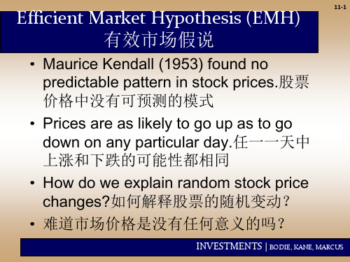
Chapter 11The Efficient Market HypothesisMultiple Choice Questions1. If you believe in the ________ form of the EMH, you believe that stock prices reflect all relevant information including historical stock prices and current public information about the firm, but not information that is available only to insiders.A.Semistrong2. When Maurice Kendall examined the patterns of stock returns in 1953 he concluded that the stock market was __________. Now, these random price movements are believed to be _________.A.inefficient; the effect of a well-functioning market3. The stock market follows a __________.B.Submartingale4. A hybrid strategy is one where the investorD.maintains a passive core and augments the position with an actively managed portfolio.5. The difference between a random walk and a submartingale is the expected price change in a random walk is ______ and the expected price change for a submartingale is ______.D.zero; positive6.6. The difference between a random walk and a submartingale is the expected price change in a random walk is ______ and the expected price change for asubmartingale is ______.D.zero; positive7. Proponents of the EMH typically advocateB.investing in an index fund.C. a passive investment strategy.E. B and C8. Proponents of the EMH typically advocateC. a passive investment strategy.9. If you believe in the _______ form of the EMH, you believe that stock prices reflect all information that can be derived by examining market trading data such as the history of past stock prices, trading volume or short interest.C.Weak10. If you believe in the _________ form of the EMH, you believe that stock prices reflect all available information, including information that is available only to insiders.B.strong11. If you believe in the reversal effect, you shouldC.buy stocks this period that performed poorly last period.12. __________ focus more on past price movements of a firm's stock than on the underlying determinants of future profitability.D.Technical analysts13. _________ above which it is difficult for the market to rise.B.Resistance level is a value14. _________ below which it is difficult for the market to fall.C.Support level is a value15. ___________ the return on a stock beyond what would be predicted from market movements alone.A.An excess economic return isC.An abnormal return isE. A and C16. The debate over whether markets are efficient will probably never be resolved because of ________.A.the lucky event issue.B.the magnitude issue.C.the selection bias issue.D.all of the above.17. A common strategy for passive management is ____________.A.creating an index fund18. Arbel (1985) found thatA.the January effect was highest for neglected firms.19. Researchers have found that most of the small firm effect occursD.in January.20. Basu (1977, 1983) found that firms with low P/E ratiosA.earned higher average returns than firms with high P/E ratios.21. Jaffe (1974) found that stock prices _________ after insiders intensively bought shares.C.increased22. Banz (1981) found that, on average, the risk-adjusted returns of small firmsA.were higher than the risk-adjusted returns of large firms.23. Proponents of the EMH think technical analystsE.are wasting their time.24. Studies of positive earnings surprises have shown that there isA. a positive abnormal return on the day positive earnings surprises are announced.B. a positive drift in the stock price on the days following the earnings surprise announcement.D.both A and B are true.25. Studies of negative earnings surprises have shown that there isA. a negative abnormal return on the day negative earnings surprises are announced.B. a positive drift in the stock price on the days following the earnings surprise announcement.D.both A and B are true.26. Studies of stock price reactions to news are calledB.event studies.27. On November 22, 2005 the stock price of Walmart was $ and the retailer stock index was . On November 25, 2005 the stock price of Walmart was $ and the retailer stock index was . Consider the ratio of Walmart to the retailer index on November 22 and November 25. Walmart is _______ the retail industry and technical analysts who follow relative strength would advise _______ the stock.A.outperforming, buying28. Work by Amihud and Mendelson (1986,1991)A.argues that investors will demand a rate of return premium to invest in less liquid stocks.B.may help explain the small firm effect.C.may be related to the neglected firm effect.E.A, B, and C.29. Fama and French (1992) found that the stocks of firms within the highest decile of market/book ratios had average monthly returns of _______ while the stocks of firms within the lowest decile of market/book ratios had average monthly returns of ________.C.less than 1%, greater than 1%30. A market decline of 23% on a day when there is no significant macroeconomic event ______ consistent with the EMH because ________.D.would not be, it was not a clear response to macroeconomic news.31. In an efficient market, __________.A.security prices react quickly to new informationB.security prices are seldom far above or below their justified levelsC.security analysts will not enable investors to realize superior returns consistentlyE.A, B, and C32. The weak form of the efficient market hypothesis asserts thatB.future changes in stock prices cannot be predicted from past prices.C.technicians cannot expect to outperform the market.E. B and C33. A support level is the price range at which a technical analyst would expect theC.demand for a stock to increase substantially.34. A finding that _________ would provide evidence against the semistrong form of the efficient market theory.A.low P/E stocks tend to have positive abnormal returnsC.one can consistently outperform the market by adopting the contrarian approach exemplified by the reversals phenomenonE. A and C35. The weak form of the efficient market hypothesis contradictsD.technical analysis, but is silent on the possibility of successful fundamental analysis. 36. Two basic assumptions of technical analysis are that security prices adjustC.gradually to new information and market prices are determined by the interaction of supply and demand.37. Cumulative abnormal returns (CAR)A.are used in event studies.B.are better measures of security returns due to firm-specific events than are abnormal returns (AR).D. A and B.38. Studies of mutual fund performanceA.indicate that one should not randomly select a mutual fund.B.indicate that historical performance is not necessarily indicative of future performance.D. A and B.39. The likelihood of an investment newsletter's successfully predicting the direction of the market for three consecutive years by chance should beC.between 10% and 25%.40. In an efficient market the correlation coefficient between stock returns for two non-overlapping time periods should beC.zero.41. The weather report says that a devastating and unexpected freeze is expected to hit Florida tonight, during the peak of the citrus harvest. In an efficient market one would expect the price of Florida Orange's stock toA.drop immediately.42. Matthews Corporation has a beta of . The annualized market return yesterday was 13%, and the risk-free rate is currently 5%. You observe that Matthews had an annualized return yesterday of 17%. Assuming that markets are efficient, this suggests thatB.good news about Matthews was announced yesterday.43. Nicholas Manufacturing just announced yesterday that its 4th quarter earnings will be 10% higher than last year's 4th quarter. You observe that Nicholas had an abnormal return of % yesterday. This suggests thatC.investors expected the earnings increase to be larger than what was actually announced.44. When Maurice Kendall first examined stock price patterns in 1953, he found thatB.there were no predictable patterns in stock prices.45. If stock prices follow a random walkD.price changes are random.46. The main difference between the three forms of market efficiency is thatD.the definition of information differs.47. Chartists practiceA.technical analysis.48. Which of the following are used by fundamental analysts to determine proper stock pricesI) trendlinesII) earningsIII) dividend prospectsIV) expectations of future interest ratesV) resistance levelsC.II, III, and IV49. According to proponents of the efficient market hypothesis, the best strategy for a small investor with a portfolio worth $40,000 is probably to E.invest in mutual funds.50. Which of the following are investment superstars who have consistently shown superior performanceI) Warren BuffetII) Phoebe BuffetIII) Peter LynchIV) Merrill LynchV) Jimmy BuffetC.I and III51. Google has a beta of . The annualized market return yesterday was 11%, and the risk-free rate is currently 5%. You observe that Google had an annualized return yesterday of 14%. Assuming that markets are efficient, this suggests thatB.good news about Google was announced yesterday.52. Music Doctors has a beta of . The annualized market return yesterday was 12%, and the risk-free rate is currently 4%. You observe that Music Doctors had an annualized return yesterday of 15%. Assuming that markets are efficient, this suggests thatA.bad news about Music Doctors was announced yesterday.53. QQAG has a beta of . The annualized market return yesterday was 13%, and the risk-free rate is currently 3%. You observe that QQAG had an annualized return yesterday of 20%. Assuming that markets are efficient, this suggests that C.no significant news about QQAG was announced yesterday.54. QQAG just announced yesterday that its 4th quarter earnings will be 35% higher than last year's 4th quarter. You observe that QQAG had an abnormal return of % yesterday. This suggests thatC.investors expected the earnings increase to be larger than what was actually announced.55. LJP Corporation just announced yesterday that it would undertake an international joint venture. You observe that LJP had an abnormal return of 3% yesterday. This suggests thatD.investors view the international joint venture as good news.56. Music Doctors just announced yesterday that its 1st quarter sales were 35% higher than last year's 1st quarter. You observe that Music Doctors had an abnormal return of -2% yesterday. This suggests thatC.investors expected the sales increase to be larger than what was actually announced.57. The Food and Drug Administration (FDA) just announced yesterday that they would approve a new cancer-fighting drug from King. You observe that King had an abnormal return of 0% yesterday. This suggests thatD.the approval was already anticipated by the market58. Your professor finds a stock-trading rule that generates excessrisk-adjusted returns. Instead of publishing the results, she keeps the trading rule to herself. This is most closely associated with ________.B.selection bias59. At freshman orientation, 1,500 students are asked to flip a coin 20 times. One student is crowned the winner (tossed 20 heads). This is most closely associated with ________.D.the lucky event issue60. Sehun (1986) finds that the practice of monitoring insider trade disclosures, and trading on that information, would be ________.E.not sufficiently profitable to cover trading costs61. If you believe in the reversal effect, you shouldC.sell stocks this period that performed well last period.62. Patell and Woflson (1984) report that most of the stock price response to corporate dividend or earnings announcements occurs within ____________ of the announcement.C. 2 hoursShort Answer Questions63. Discuss the various forms of market efficiency. Include in your discussion the information sets involved in each form and the relationships across information sets and across forms of market efficiency. Also discuss the implications for the various forms of market efficiency for the various types of securities' analysts.The weak form of the efficient markets hypothesis (EMH) states that stock prices immediately reflect market data. Market data refers to stock prices and trading volume. Technicians attempt to predict future stock prices based on historic stock price movements. Thus, if the weak form of the EMH holds, the work of the technician is of no value.The semistrong form of the EMH states that stock prices include all public information. This public information includes market data and all other publicly available information, such as financial statements, and all information reported in the press relevant to the firm. Thus, market information is a subset of all public information. As a result, if the semistrong form of the EMH holds, the weak form must hold also. If the semistrong form holds, then the fundamentalist, who attempts to identify undervalued securities by analyzing public information, is unlikely to do so consistently over time. In fact, the work of the fundamentalist may make the markets even more efficient!The strong form of the EMH states that all information (public and private) is immediately reflected in stock prices. Public information is a subset of all information, thus if the strong form of the EMH holds, the semistrong form must hold also. The strong form of EMH states that even with inside (legal or illegal) information, one cannot expect to outperform the market consistently over time. Studies have shown the weak form to hold, when transactions costs are considered. Studies have shown the semistrong form to hold in general, although some anomalies have been observed. Studies have shown that some insiders (specialists, major shareholders, major corporate officers) do outperform the market. Feedback: The purpose of this question is to assure that the student understands the interrelationships across different forms of the EMH, across the informationsets, and the implications of each form for different types of analysts.64. What is an event study It is a test of what form of market efficiency Discuss the process of conducting an event study, including the best variable(s) to observe as tests of market efficiency.A event study is an empirical test which allows the researcher to assess the impact of a particular event on a firm's stock price. To do so, one often uses the index model and estimates e, the residual term which measures thetfirm-specific component of the stock's return. This variable is the difference between the return the stock would ordinarily earn for a given level of market performance and the actual rate of return on the stock. This measure is often referred to as the abnormal return of the stock. However, it is very difficult to identify the exact point in time that an event becomes public information; thus, the better measure is the cumulative abnormal return, which is the sum of abnormal returns over a period of time (a window around the event date). This technique may be used to study the effect of any public event on a firm's stock price; thus, this technique is a test of the semistrong form of the EMH. Feedback: The rationale for this question is to ascertain if the student understands the methodology most commonly used as a test of the semistrong form of market efficiency.65. Discuss the small firm effect, the neglected firm effect, and the January effect, the tax effect and how the four effects may be related.Studies have shown that small firms earn a risk-adjusted rate of return greater than that of larger firms. Additional studies have shown that firms that are not followed by analysts (neglected firms) also have a risk-adjusted return greater than that of larger firms. However, the neglected firms tend to be small firms; thus, the neglected firm effect may be a manifestation of the small firm effect. Finally, studies have shown that returns in January tend to be higher than in other months of the year. This effect has been shown to persist consistently over the years. However, the January effect may be the tax effect, as investors may have sold stocks with losses in December for tax purposes and reinvested in January. Small firms (and neglected firms) would tend to be more affected by this increased buying than larger firms, as small firms tend to sell for lower prices.Feedback: The purpose of this question is to reinforce the interrelationships, that "effects" may not always be independent and thus readily identifiable. Also these effects are widely discussed in the financial press, and the January effect appears to be quite persistent.66. Why might the degree of market efficiency differ across various markets State three reasons why this might occur and explain each reason briefly.1. Market efficiency depends on information being essentially free and costless to market participants. In the . markets this is the case to a large extent. The . markets are well developed and professional analysts often follow securities. Information is available on television, in the press, and on the Internet. The opposite may be true in other markets, such as those of developing countries, where there are fewer or no analysts and few market participants with these resources.2. Accounting disclosure requirements are different across markets. In the . firms must meet SEC requirements to be publicly traded. In other countries the requirements may be different or nonexistent. This has implications about the ease with which analysts can evaluate the company to determine its proper value.3. Markets for "neglected" stocks may be less efficient than markets for stocks that are heavily followed by analysts. If analysts feel that it is not worthwhile to give their attention to particular stocks then ample information about these stocks will not be readily available to investors.Feedback: This question leads the student to look at some of the fundamental reasons for market efficiency and why there may be differences among markets with regard to the reasons. Alternative answers are possible.67. With regard to market efficiency, what is meant by the term "anomaly" Give three examples of market anomalies and explain why each is considered to be an anomaly.Anomalies are patterns that should not exist if the market is truly efficient. Investors might be able to make abnormal profits by exploiting the anomalies, which doesn't make sense in an efficient market.Possible examples include, but are not limited to, the following.the small-firm effect - average annual returns are consistently higher for small-firm portfolios, even when adjusted for risk by using the CAPM.January effect - the small-firm effect occurs virtually entirely in January. neglected-firm effect - small firms tend to be ignored by large institutional traders and stock analysts. This lack of monitoring makes them riskier and they earn higher risk-adjusted returns. The January effect is largest for neglected firms.the liquidity effect - investors demand a return premium to invest in less-liquid stocks. This is related to the small-firm effect and the neglected-firm effect. These stocks tend to earn high risk-adjusted rates of return.ratios - firms with the higher book-to-market-value ratios have higherrisk-adjusted returns, suggesting that they are underpriced. When combined with the firm-size factor, this ratio explained returns better than systematic risk as measured by beta.the reversal effect - stocks that have performed best in the recent past seem to underperform the rest of the market in the following periods, and vice versa. Other studies indicated that this effect might be an illusion. These studies used portfolios formed mid-year rather than in December and considered the liquidity effect.Investors should not be able to earn excess returns by taking advantage of anyof these. The market should adjust prices to their proper levels. But these things have been documented to occur repeatedly.Feedback: This question tests whether the student grasps the basic concept of anomalies and allows some choice in explaining some of them.。

Chapter17Macroeconomic and industry Analysis1. A top down analysis of a firm starts with ____________.D. the global economy2. An example of a highly cyclical industry is ________.A. the automobile industry3. Demand-side economics is concerned with _______.A. government spending and tax levelsB. monetary policyC. fiscal policyE. A, B, and C4. The most widely used monetary tool is ___________.C. open market operations5. The "real", or inflation-adjusted, exchange rate, isC. the purchasing power ratio.6. The "normal" range of price-earnings ratios for the S&P 500 Index isD. between 12 and 257. Monetary policy is determined byC. the board of Governors of the Federal Reserve System.8. A trough is ________.B. a transition from a contraction in the business cycle to the start of an expansion9. A peak is ________.A. a transition from an expansion in the business cycle to the start of a contraction10. If the economy is growing, firms with high operating leverage will experience __________.A. higher increases in profits than firms with low operating leverage.11. If the economy is shrinking, firms with high operating leverage will experience __________.A. higher decreases in profits than firms with low operating leverage.12. If the economy is growing, firms with low operating leverage will experience __________.C. smaller increases in profits than firms with high operating leverage.13. If the economy is shrinking, firms with low operating leverage will experience__________.C. smaller decreases in profits than firms with high operating leverage.14. Industrial production refers to _________.C. the total manufacturing output in the economy.15. GDP refers to _________.D. the total production of goods and services in the economy16. A rapidly growing GDP indicates a(n) ______ economy with ______ opportunity for a firm to increase sales.D. expanding; ample17. A declining GDP indicates a(n) ______ economy with ______ opportunity for a firm to increase sales.A. stagnant; little18. The average duration of unemployment and changes in the consumer price index for services are _________.C. lagging economic indicators19. A firm in an industry that is very sensitive to the business cycle will likely have a stock beta ___________.A. greater than 1.020. If the economy were going into a recession, an attractive industry to invest in would be the ________ industry.B. medical services21. The stock price index and contracts and new orders for nondefense capital goods areA. leading economic indicators.22. A firm in the early stages of the industry life cycle will likely have ________.B. high risk.C. rapid growthE. B and C23. Assume the U.S. government was to decide to increase the budget deficit. This action will most likely cause __________ to increaseA. interest ratesB. government borrowingD. both A and B24. Assume the U.S. government was to decide to decrease the budget deficit. This action will most likely cause __________ to decreaseA. interest ratesB. government borrowingD. both A and B25. Assume that the Federal Reserve decreases the money supply. This action will cause________ to decrease.C. investment in the economy26. If the currency of your country is depreciating, the result should be to ______ exports and to _______ imports.B. stimulate, discourage27. If the currency of your country is appreciating, the result should be to ______ exports and to _______ imports.C. discourage, stimulate28. Increases in the money supply will cause demand for investment and consumption goods to _______ in the short run and cause prices to ________ in the long run.A. increase, increase29. The North American Industry Classification System (NAICS)A. are for firms that operate in the NAFTA region.B. group firms by industry.D. A and B.30. If interest rates increase, business investment expenditures are likely to ______ and consumer durable expenditures are likely to _________.D. decrease, decrease31. Fiscal policy generally has a _______ direct impact than monetary policy on the economy, and the formulation and implementation of fiscal policy is ______ than that of monetary policy.B. more, slower32. Fiscal policy is difficult to implement quickly becauseA. it requires political negotiations.B. much of government spending is nondiscretionary and cannot be changed.D. A and B.33. InflationA. is the rate at which the general level of prices is increasing.B. rates are high when the economy is considered to be "overheated".D. A and B.Two firms, A and B, both produce widgets. The price of widgets is $1 each. Firm A has total fixed costs of $500,000 and variable costs of 50 cents per widget. Firm B has total fixed costs of $240,000 and variable costs of 75 cents per widget. The corporate tax rate is 40%. If the economy is strong, each firm will sell 1,200,000 widgets. If the economy enters a recession, each firm will sell 1,100,000 widgets.34. If the economy enters a recession, the after-tax profit of Firm A will be ________.C. $30,00035. If the economy enters a recession, the after-tax profit of Firm B will be _______.E. none of the above36. If the economy is strong, the after-tax profit of Firm A will be _______.D. $60,00037. If the economy is strong, the after-tax profit of Firm B will be __________.C. $36,00038. Calculate firm A's degree of operating leverage.A. 11.039. Calculate firm B's degree of operating leverage.C. 29.8640. Classifying firms into groups, such as _________ provides an alternative to the industry life cycle.A. slow-growersB. stalwartsD. A and B41. Supply-side economists wishing to stimulate the economy are most likely to recommendD. a decrease in the tax rate.42. Which of the following are not examples of defensive industries?B. durable goods producers.43. Which of the following are examples of defensive industries?A. food producers.C. pharmaceutical firms.D. public utilitiesE. A, C and D44. ________ is a proposition that a strong proponent of supply side economics would most likely stress.B. Higher marginal tax rates promote economic inefficiency and thereby retard aggregate output as they encourage investors to undertake low productivity projects with substantial tax shelter benefits45. The industry life cycle is described by which of the following stage(s)?A. start-up.B. consolidation.D. A and B.46. In the start-up stage of the industry life cycleA. it is difficult to predict which firms will succeed and which firms will fail.B. industry growth is very rapid.D. A and B.47. In the consolidation stage of the industry life-cycleC. the performance of firms will more closely track the performance of the overall industry.48. In the maturity stage of the industry life cycleA. the product has reached full potential.B. profit margins are narrower.C. producers are forced to compete on price to a greater extent.E. A, B, and C.49. In the decline stage of the industry life cycleA. the product may have reached obsolescence.B. the industry will grow at a rate less than the overall economy.C. the industry may experience negative growth.E. A, B, and C.50. A variety of factors relating to industry structure affect the performance of the firm, includingA. threat of entry.B. rivalry between existing competitors.E. A and B.51. The process of estimating the dividends and earnings that can be expected from the firm based on determinants of value is calledD. fundamental analysis.52. The emerging market exhibiting the highest growth in real GDP in 2007 wasA. China53. The emerging stock market exhibiting the highest U.S. dollar return in 2007 wasA. China54. The life cycle stage in which industry leaders are likely to emerge is theC. consolidation stage.55. Investment manager Peter Lynch refers to firms that are in bankruptcy or soon might be asE. turnarounds.56. A top-down analysis of a firm's prospects starts withD. an assessment of the broad economic environment.57. Over the period 1999-2006, which of the following countries had a change in its real exchange rate that was favorable for U.S. consumers who want to buy its goods?E. Japan58. Over the period 1999-2006, which of the following countries had a change in its real exchange rate that was most unfavorable for U.S. consumers who want to buy its goods?A. Canada59. In recent years, P/E multiples haveB. risen dramatically.60. In recent years, P/E multiples for S&P 500 companies haveD. ranged from 12 to 25.61. The industry with the highest ROE in 2007 wasD. iron/steel.62. The industry with the lowest ROE in 2007 wasE. airlines.63. The industry with the lowest return in 2007 wasA. home construction.64. The industry with the highest return in 2007 wasB. oil equipment.65. Investors can ______ invest in an industry with the highest expected return by purchasing ______.B. not; industry-specific iShares66. Which of the following are key economic statistics that are used to describe the state of the macroeconomy?I) gross domestic productII) the unemployment rateIII) inflationIV) consumer sentimentV) the budget deficitE. I, II, III, IV, and V67. An example of a positive demand shock isE. a decrease in tax rates.68. An example of a negative demand shock isA. a decrease in the money supply.B. a decrease in government spending.E. A and B.69. During which stage of the industry life cycle would a firm experience stable growth in sales?A. Consolidation70. The emerging stock market exhibiting the highest local currency return in 2007 wasB. ChinaE. China71. Sector rotationC. is shifting the portfolio more heavily toward an industry or sector that is expected to perform well in the future.72. According to Michael Porter, there are five determinants of competition. An example of _____ is when new entrants to an industry our pressure on prices and profits.A. Threat of Entry73. According to Michael Porter, there are five determinants of competition. An example of _____ is when competitors seek to expand their share of the market.B. Rivalry between Existing Competitors74. According to Michael Porter, there are five determinants of competition. An example of _____ is when the availability limits the prices that can be charged to customers.C. Pressure from Substitute Products75. According to Michael Porter, there are five determinants of competition. An example of _____ is when a buyer purchases a large fraction of an industry's output and can demand price concessions.D. Bargaining power of Buyers76. Assume the U.S. government was to decide to increase the budget deficit. This action will most likely cause __________ to increaseA. interest ratesB. government borrowingD. both A and B77. If interest rates decrease, business investment expenditures are likely to ______ and consumer durable expenditures are likely to _________.A. increase, increase78. An example of a defensive industry is ________.B. the tobacco industryC. the food industryE. B and CTwo firms, C and D, both produce coat hangers. The price of coat hangers is $1.20 each. Firm C has total fixed costs of $750,000 and variable costs of 30 cents per widget. Firm D has total fixed costs of $400,000 and variable costs of 50 cents per widget. The corporate tax rate is 40%. If the economy is strong, each firm will sell 2,000,000 widgets. If the economy enters a recession, each firm will sell 1,400,000 widgets.79. If the economy enters a recession, the total revenue of Firm C will be ________.A. $1,680,00080. If the economy enters a recession, the total cost of Firm C will be ________.B. $1,170,00081. If the economy enters a recession, the before tax profit of Firm C will be ________.C. $510,00082. If the economy enters a recession, the tax of Firm C will be ________.D. $204,00083. If the economy enters a recession, the after tax profit of Firm C will be ________.E. $306,00084. If the economy is strong, the total revenue of Firm C will be ________.D. $2,400,00085. If the economy is strong, the total cost of Firm C will be ________.C. $1,305,00086. If the economy is strong, the before tax profit of Firm C will be ________.B. $1,050,00087. If the economy is strong, the tax of Firm C will be ________.A. $420,00088. If the economy is strong, the after-tax profit of Firm C will be _______.E. $630,00089. If a firm's sales decrease by 15% and profits decrease by 20% during a recession, the firms operating leverage is ____________?A. 1.33Short Answer Questions90. Discuss the tools of the U.S. government's "demand-side" policy. Include in your discussion of these tools the relative advantages and disadvantages of each in terms of the effect of the use of these tools on the economy.The two tools of the government's "demand-side" policy are fiscal and monetary policy. Fiscal policy is the use of government spending and taxing for the specific purpose of stabilizing the economy. Fiscal policy, once enacted, has the most direct and immediate effect on the economy. However, the formulation and implementation of fiscal policy is extremely slow, as such policy must be approved by both the legislative and executive branches of the federal government. Monetary policy consists of actions taken by the Board of Governors of the Federal Reserve System (FRS) to influence the money supply and/or interest rates. Monetary policy is relatively easy to formulate and to implement, but has less direct impact on the economy than fiscal policy. The most widely used tool of the FRS is the open market operations, in which the Fed buys or sells bonds for the Fed's account. Buying securities increases the money supply; selling securities decreases the money supply. Open market operations occur daily. Other FRS tools include adjusting the discount rate, which is the interest rate the Fed charges banks onshort-term loans, and altering reserve requirements, which are the fraction of deposits that banks must maintain in cash deposits with the Fed. Reductions in the money supply signal an expansionary monetary policy; lowering reserve requirements increase the money supply, and thus, stimulate the economy. The Fed walks a fine line: expansionary monetary policy probably will lower interest rates and stimulate investment and consumption in the short run, but ultimately inflation probably will result.Feedback: The rationale of this question is to ascertain whether the student has an understanding of the basic principles of macroeconomics.91. Discuss the National Bureau of Economic Research (NBER)'s indexes of economic indicators, and how each of the categories of these indicators might be used by the securities' analyst.The NBER has developed a set of cyclical indicators to help forecast, measure, and interpret short-term fluctuations in economic activity. The leading economic indicators are those that tend to increase or decrease in advance of the rest of the economy. These indicators are used to forecast the state of the economy for the coming period (usually one year). Coincident economic indicators move in tandem with the broad economy, and are used to confirm (or disconfirm) an earlier economic prediction. Lagging economic indicators are those that move after the broad economy, and are used to identify the end of a stage of the business cycle (such as a trough) and as an indication that another stage of business cycle (such as the expansion) is about to begin. The S&P 500 stock index is an excellent leading economic indicator, as would be expected by market efficiency proponents. However, if the stock market anticipates general economic trends, the task of the fundamentalist using economic forecasts to identify attractive industries (and thus stocks) for the future becomes even more impossible.Feedback: The purpose of this question is to ascertain the student's understanding of the widely quoted economic indicators and the usefulness (and lack thereof) in securities' analysis.92. Discuss the industry life cycle, how this concept can be used by security analysts, and the limitations of this concept for security analysis.The industry life cycle may be defined by the following stages: start up (rapid and increasing growth), consolidation (sable growth), maturity (slowing growth), and relative decline (minimal or negative growth). Investors interested in identifying new, and presumably ultimately successful, industries will use this technique, trying to get in on the "ground floor". In the start up stage, no historical data is present; thus, one cannot identify potentially successful firms. However, typically, all of the firms are selling at low prices and the investor will "diversify across the industry" by buying many different stocks in the industry. If the industry becomes successful, the surviving firms will appreciate substantially in value; the non-surviving firms will be written off as losses. Typically, in this stage, firms are paying little or no dividends. Investment in this stage is for the risk-tolerant investor. As the industry moves from the start up to the consolidation stage, firms begin paying or increasing dividends; the surviving firms become more successful, begin to enjoy economies of scale, and are moving up the learning curve in terms of cost efficiency. In the maturity stage, the growth has slowed and dividends may have increased; less risk is involved. By the relative decline stage, the firm has no new exciting capital budgeting projects and may have become an "income stock", by paying out a higher than average level of dividends. At this stage, the stock may be attractive for the risk-averse retiree interested in dividend income. However, the stock must be watched carefully in this stage, as this industry may be dying (buggy whips). However, over the industry life cycle, the clientele for the firms' stocks have changed, from the risk-tolerant to the risk averse.The problem with using this concept for investment purposes is identifying where the industry is in the industry life cycle. In addition, all industries do not move through the cycle in the same fashion. In fact, the goal is to avoid the relative decline stage.Feedback: The purpose of this question is to ascertain whether the student understands the industry life cycle, how the concept can be used by investors, and the limitations of the concept for investors.93. Discuss the ways in which the global economy might have an effect on a firm whose headquarters are in Montana. Be specific - cite some of the relevant factors that should be considered.A firm that operates from Montana cannot ignore the global economy. The firm may make sales to other countries, employ people from other countries, and invest in other countries. It may face price competition from similar firms abroad, be subject to wages that are different from those paid by foreign firms, and management may have less power to do what it wants due to labor unions. Exports of its products and imports will be influenced by the global economy. Interest rates in other countries will determine part of the return on the firm's investments. Exchange rates pose an additional risk if the company wants to repatriate its earnings. Countries' political and economic policies should be considered, with some being more predictable than others. Global markets have some linkages, but there are significant variations in performance among countries.Feedback: This question emphasizes the importance of the global economy, which should not be ignored when doing a macroeconomic analysis.94. List and discuss three of the five determinants of competition suggested in Porter's 1985 study.The determinants are: the threat of entry from new competitors, rivalry between existing competitors, price pressure from substitute products, the bargaining power of buyers, and the bargaining power of suppliers. Each of these is discussed below.Threat of entry from new competitors - If there are high profit margins in the industry, new competitors will be likely to enter. There may be some barriers to entry that existing firms can establish to discourage this. Possible barriers include longstanding relationships with suppliers and buyers, proprietary knowledge or patents, brand loyalty, and experience in the market. Rivalry between existing competitors - This could lead to price competition and lower profit margins. Expansion of one firm cuts into the rivals' market shares. Firms with homogeneous products face price pressure because they are unable to differentiate their products from their competitors' products. High fixed costs might force a company to operate at close to full capacity.Price pressure from substitute products - If firms in related industries produce similar products, the firm may not be able to charge as much for its product. Some examples are carbonated beverages and fruit drinks, paint and wallpaper, and movies and videos. Many other examples may be offered.Bargaining power of buyers - Buyers might have bargaining power if they purchase a substantial proportion of the firm's output. The firm might have to settle for accepting a lower price for its products. The automobile industry is an example given in the textbook. Bargaining power of suppliers - If the firm depends on a supplier to provide much of its inputs, the supplier might demand a higher price. This is especially true if there are no easily available alternative suppliers. Labor unions are cited as an example.Feedback: This question tests the student's understanding of the relationships among industry structure, competitive strategy, and profitability.。

英语作文-医学护肤品制造行业的价格策略与市场定价分析方法The pricing strategy and market pricing analysis methods in the medical skincare product manufacturing industry are crucial for companies to effectively compete and thrive in the market. In this highly competitive industry, companies need to carefully consider their pricing strategies to attract customers, maintain profitability, and stay ahead of the competition.One of the key pricing strategies in the medical skincare product manufacturing industry is value-based pricing. This strategy involves setting prices based on the value that customers perceive in the product. Companies need to understand the needs and preferences of their target customers and position their products as offering unique value compared to competitors. By pricing their products based on the value they provide to customers, companies can justify higher prices and differentiate themselves in the market.Another important pricing strategy in the medical skincare product manufacturing industry is cost-based pricing. This strategy involves setting prices based on the costs of manufacturing, distributing, and marketing the product, as well as desired profit margins. Companies need to carefully calculate their costs and factor in all expenses to ensure that they are pricing their products profitably. By using cost-based pricing, companies can ensure that they are covering their expenses and generating a reasonable profit margin.In addition to value-based and cost-based pricing, companies in the medical skincare product manufacturing industry can also use competitive pricing strategies. This involves setting prices based on the prices of competitors in the market. Companies need to carefully monitor the prices of competitors and adjust their own prices accordingly to remain competitive. By offering competitive prices, companies can attract price-sensitive customers and gain market share.When analyzing market pricing, companies in the medical skincare product manufacturing industry need to consider various factors, such as customer demographics,market trends, and competitor pricing strategies. By conducting market research and analyzing market data, companies can gain valuable insights into customer preferences and behaviors, as well as market dynamics. This information can help companies develop pricing strategies that are tailored to the needs of their target customers and aligned with market trends.Overall, the pricing strategy and market pricing analysis methods in the medical skincare product manufacturing industry play a critical role in the success of companies. By carefully considering factors such as value, costs, competition, and market trends, companies can develop pricing strategies that attract customers, maintain profitability, and achieve long-term success in the market.。