神经网络控制01 (英文)
- 格式:doc
- 大小:396.50 KB
- 文档页数:51

人工神经网络控制摘要: 神经网络控制,即基于神经网络控制或简称神经控制,是指在控制系统中采用神经网络这一工具对难以精确描述的复杂的非线性对象进行建模,或充当控制器,或优化计算,或进行推理,或故障诊断等,亦即同时兼有上述某些功能的适应组合,将这样的系统统称为神经网络的控制系统。
本文从人工神经网络,以及控制理论如何与神经网络相结合,详细的论述了神经网络控制的应用以及发展。
关键词: 神经网络控制;控制系统;人工神经网络人工神经网络的发展过程神经网络控制是20世纪80年代末期发展起来的自动控制领域的前沿学科之一。
它是智能控制的一个新的分支,为解决复杂的非线性、不确定、不确知系统的控制问题开辟了新途径。
是(人工)神经网络理论与控制理论相结合的产物,是发展中的学科。
它汇集了包括数学、生物学、神经生理学、脑科学、遗传学、人工智能、计算机科学、自动控制等学科的理论、技术、方法及研究成果。
在控制领域,将具有学习能力的控制系统称为学习控制系统,属于智能控制系统。
神经控制是有学习能力的,属于学习控制,是智能控制的一个分支。
神经控制发展至今,虽仅有十余年的历史,已有了多种控制结构。
如神经预测控制、神经逆系统控制等。
生物神经元模型神经元是大脑处理信息的基本单元,人脑大约含1012个神经元,分成约1000种类型,每个神经元大约与102~104个其他神经元相连接,形成极为错综复杂而又灵活多变的神经网络。
每个神经元虽然都十分简单,但是如此大量的神经元之间、如此复杂的连接却可以演化出丰富多彩的行为方式,同时,如此大量的神经元与外部感受器之间的多种多样的连接方式也蕴含了变化莫测的反应方式。
图1生物神经元传递信息的过程为多输入、单输出,神经元各组成部分的功能来看,信息的处理与传递主要发生在突触附近,当神经元细胞体通过轴突传到突触前膜的脉冲幅度达到一定强度,即超过其阈值电位后,突触前膜将向突触间隙释放神经传递的化学物质,突触有两种类型,兴奋性突触和抑制性突触。

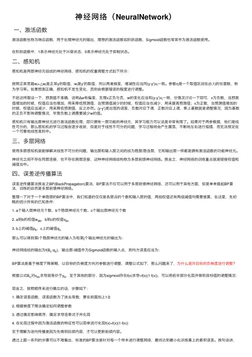
神经⽹络(NeuralNetwork)⼀、激活函数激活函数也称为响应函数,⽤于处理神经元的输出,理想的激活函数如阶跃函数,Sigmoid函数也常常作为激活函数使⽤。
在阶跃函数中,1表⽰神经元处于兴奋状态,0表⽰神经元处于抑制状态。
⼆、感知机感知机是两层神经元组成的神经⽹络,感知机的权重调整⽅式如下所⽰:按照正常思路w i+△w i是正常y的取值,w i是y'的取值,所以两者做差,增减性应当同(y-y')x i⼀致。
参数η是⼀个取值区间在(0,1)的任意数,称为学习率。
如果预测正确,感知机不发⽣变化,否则会根据错误的程度进⾏调整。
不妨这样假设⼀下,预测值不准确,说明Δw有偏差,⽆理x正负与否,w的变化应当和(y-y')x i⼀致,分情况讨论⼀下即可,x为负数,当预测值增加的时候,权值应当也增加,⽤来降低预测值,当预测值减少的时候,权值应当也减少,⽤来提⾼预测值;x为正数,当预测值增加的时候,权值应当减少,⽤来降低预测值,反之亦然。
(y-y')是出现的误差,负数对应下调,正数对应上调,乘上基数就是调整情况,因为基数的正负不影响调整情况,毕竟负数上调需要减少w的值。
感知机只有输出层神经元进⾏激活函数处理,即只拥有⼀层功能的神经元,其学习能⼒可以说是⾮常有限了。
如果对于两参数据,他们是线性可分的,那么感知机的学习过程会逐步收敛,但是对于线性不可分的问题,学习过程将会产⽣震荡,不断地左右进⾏摇摆,⽽⽆法恒定在⼀个可靠地线性准则中。
三、多层⽹络使⽤多层感知机就能够解决线性不可分的问题,输出层和输⼊层之间的成为隐层/隐含层,它和输出层⼀样都是拥有激活函数的功能神经元。
神经元之间不存在同层连接,也不存在跨层连接,这种神经⽹络结构称为多层前馈神经⽹络。
换⾔之,神经⽹络的训练重点就是链接权值和阈值当中。
四、误差逆传播算法误差逆传播算法换⾔之BP(BackPropagation)算法,BP算法不仅可以⽤于多层前馈神经⽹络,还可以⽤于其他⽅⾯,但是单单提起BP算法,训练的⾃然是多层前馈神经⽹络。

Study on the Managing System of Fees Collecting by WaterMeter Based on CPU CardHUA Xiang-gang LIAN Xiao-gin WU Ye-lanABSTRACT:This paper introduces a managing system of fees coiiecting by water meter based on CPU card,shows the generai structure of this system,and expounds the functions of its main compositions and the concrete reaiization of these functions.KEY WORDS:CPU card;water meter;fees coiiecting system;information management system成用户卡密钥派生功能。
(4)总控卡。
总控卡密藏一个由发卡方相关人员产生的主控密钥,这个总控密钥通过和特定代码做加密运算产生水表SAM 模块,发行SAM 卡等的主工作密钥。
(5)检查卡。
主要在现场或生产过程中对水表的数据进行检查核对的卡片,为保证检查卡使用的方便性,检查卡对数据进行操作时不进行一卡一表的数据认证。
(6)生产数据设置卡。
主要在生产过程中对水表的参数进行设置。
(7)修改密钥卡。
用于将生产过程中使用的公开测试密钥更换为运行密钥。
(8)回收转移卡。
主要用于在现场进行换表操作时将旧表中的数据一次全部转移到新表中。
(9)校时卡。
主要用于在生产过程中或在现场运行状态下对水表中的时钟和日历进行调校。
(10)应急购水卡。
当水表内水量为零或透支状态时,用户可将应急购水卡中的购水量加入水表中以做应急使用。
由于CPU 卡具有大容量的优点,因此可在一张卡上开辟多个应用。


1, neural network information processing mathematical processNeural network information processing can be used to illustrate the mathematical process, this process can be divided into two phases; the implementation phase and learning phase. The following note to the network before the two phases.1. Implementation phaseImplementation stage is the neural network to process the input information and generates the corresponding output process. In the implementation phase, the network structure and weights of the connection is already established and will not change. Then there is:X i (t +1) = f i [u i (t +1)]Where: X i is the pre-order neurons in the output;W ij is the first i of neurons and pre-j neurons synapse weightsθ i: i neurons is the first threshold;i-f i is the neuron activation function;I X i is the output neurons.2. Learning phaseNeural network learning phase is from the sound stage; this time, the learning network according to certain rule changes synaptic weights W ij,in order to enable end fixed measure function E is minimized. General access:E = (T i, X i) (1-9)Where, T i is the teacher signal;X i is the neuron output.Learning formula can be expressed as the following mathematical expression:Where: Ψ is a nonlinear function;η ij is the weight rate of change;n is the number of iterations during learning.For the gradient learning algorithm, you can use the following specific formula:Neural networks of information processing in general need to learn and implementation phases and combined to achieve a reasonable process. Neural network learning is to obtain information on the adaptability of information, or information of the characteristics; and neural network implementation process of information is characteristic of information retrieval or classification process.Learning and neural network implementation is indispensable to the two treatment and function. Neural network behavior and the role of various effective are two key processes by which to achieve.Through the study phase, can be a pair neural network training mode is particularly sensitive information, or have some characteristics of dynamic systems. Through the implementation phase, you can use neural networks to identify the information model or feature.In intelligent control, using neural network as controller, then the neural network learning is to learn the characteristics of controlled object, so that neural network can adapt to the input-output relationship between the controlled object; Thus, in implementation, neural network will be able to learn the knowledge of an object to achieve just the right control.Second, back-propagation BP modelNeural network learning is one of the most important and most impressive features. In neural network development process, learning algorithm has a very important position. At present, people put forward neural network model and learning algorithm are appropriate. So, sometimes people do not go to pray on the model and algorithm are strict definition or distinction. Some models can have a variety of algorithms. However, some algorithms may be used for a variety of models. However, sometimes also known as the model algorithm.Since the 40's Hebb learning rule has been proposed, people have proposed a variety of learning algorithms. Among them, in 1986, proposed by Rumelhart and other back-propagation method, that is, BP (error BackPropagation) method most widely affected. Even today, BP control algorithm is still the most important application of the most effective algorithm.1.2.1 Neural network learning mechanisms and institutionsIn the neural network, the model provided on the external environment to learn the training samples, and to store this model is called sensor; ability to adapt to external environment, can automatically extract the external environmental characteristics, is called cognitive device .Neural Networks in the study, generally divided into a study of two teachers and not teachers. Sensor signal by a teacher to learn, and cognitive devicesare used to learn without teacher signals. Such as BP neural network in the main network, Hopfield network, ART network and Kohonen network; BP network and Hopfield network is necessary for teachers to learn the signal can be; and ART network and Kohonen network signals do not need teachers to learn. The so-called teacher signal, that is, learning in neural network model of sample provided by an external signal.First, the learning structure of sensorPerceptron learning is the most typical neural network learning.At present, the control application is a multilayer feedforward network, which is a sensor model, learning algorithm is BP method, it is a supervised learning algorithm.A teacher of the learning system can be expressed in Figure 1-7. This learning system is divided into three parts: input Ministry of Training Department of the Ministry and output.Input received from outside the Department of input samples X, conducted by the Training Department to adjust the network weights W, and then the Department of the output from the output. Zai this process, the desired output signal can be used as teacher signal input, by the teacher signal and the actual output Jinxingbijiao, produce the Wucha right to Kongzhixiugai系数W.Learning organization structure can be expressed as shown in Figure 1-8.In the figure, X l, X 2, ..., X n, is the input sample signals, W 1, W 2, ..., W n are weights. Input sample signal X i can take discrete values "0" or "1." Input sample signa ls weights role in the u produces the output ΣW i X i, that is:u = ΣW i X i = W 1 X 1 + W 2 X 2 + ... + W n X nThen the desired output signal Y (t) and u compare the resulting error signal e. Body weight that is adjusted according to the error e to the power factor of the learning system be modified, modify the direction of the error e should be made smaller, and constantly go on, so that the error e is zero, then the actual output value of u and the desired output value Y ( t) exactly the same, then the end of the learning process.Neural network learning generally require repeated training, error tends gradually to zero, and finally reaches zero. Then the output will be consistent with expectations. neural network learning is the consumption of a certain period, some of the learning process to be repeated many times, even up to 10 000 secondary. The reason is that neural network weights W have a lot of weight W 1, W 2 ,---- W n; that is, more than one parameter to modify the system. Adjusting the system parameters must be time-consuming consumption. At present, the neural network to improve the learning speed and reduce thenumber of repeat learn the importance of research topic is real-time control of the key issues.Second, Perceptron learning algorithmSensor is a single-layer neural network computing unit, from the linear elements and the threshold component composition. Sensor shown in Figure 1-9.Figure 1-9 Sensor structureThe mathematical model of sensor:Where: f [.] Is a step function, and thereθ is the threshold.The greatest effect sensor is able to enter the sample classificationThat is, when the sensor output to 1, the input samples as A; output is -1, the input sample as B class. From the sensor can see the classification boundaries are:Only two components in the input sample X1, X2, then a classification boundary conditions:ThatW 1 X 1 + W 2 X 2-θ = 0 (1-17)Can also be written asThen the classification as shown in solid 1-10.Perceptron learning algorithm aims to find appropriate weights w = (w1.w2, ..., Wn), the system for a particular sample x = (xt, x2, ..., xn) Bear generate expectations d. When x is classified as category A, the expected value of d = 1; X to B class, d =- 1. To facilitate the description perceptron learningalgorithm, the threshold θ and w in the human factor, while the corresponding increase in the sample x is also a component of x n +1.So that:W n +1 =- θ, X n +1 = 1 (1-19)The sensor output can be expressed as:Perceptron learning algorithm as follows:1. Set initial value of the weights wOn the weights w = (W 1. W 2, ..., W n, W n +1) of the various components of the zero set of a small random value, but W n +1 =-G. And recorded as W l (0), W 2 (0), ..., W n (0), while there Wn +1 (0) =- θ. Where W i (t) as the time from i-tEnter the weight coefficient, i = 1,2, ..., n. W n +1 (t) for the time t when the threshold.2. Enter the same as the X = (X 1, X 2, ..., X n +1) and its expected output d. Desired output value d in samples of different classes are not the same time value. If x is A class, then take d = 1, if x is B, then take -1. The desired output signal d that is, the teacher.3. Calculate the actual output value of Y4. According to the actual output error e requeste = d-Y (t) (1-21)5. With error e to modify the weightsi = 1,2, ..., n, n +1 (1-22)Where, η is called the weight change rate, 0 <η ≤ 1In equation (1-22) in, η the value can not be too much. If a value too large will affect the w i (t) stability; the value can not be too small, too small will make W i (t) the process of deriving the convergence rate is too slow.When the actual output and expected the same d are:W i (t +1) = W i (t)6. Go to point 2, has been implementing to all the samples were stable. From the above equation (1-14) known, sensor is actually a classifier, it is this classification and the corresponding binary logic. Therefore, the sensor can be used to implement logic functions. Sensor to achieve the following logic function on the situation of some description.Example: Using sensors to achieve the logic function X 1 VX 2 of the true value:To X1VX2 = 1 for the A class to X1VX2 = 0 for the B category, there are equationsThat is:From (1-24) are:W 1≥θ, W 2≥θSo that W 1 = 1, W 2 = 2Have: θ ≤ 1Take θ = 0.5There are: X1 + X2-0.5 = 0, the classification shown in Figure 1-11.Figure 1-11 Logic Function X 1 VX 2 classification1.2.2 Gradient Neural Network LearningDevice from the flu, such as the learning algorithm known, the purpose of study is on changes in the network weights, so that the network model for the input samples can be correctly classified. When the study ended, that is when the neural network correctly classified, the weight coefficient is clearly reflected in similar samples of the input common mode characteristics. In other words, weight is stored in the input mode. As the power factor is theexisting decentralized, so there is a natural neural network distributed storage features.Sensor in front of the transfer function is a step function, so it can be used as a classifier. The previous section about the Perceptron learning algorithm because of its transfer function is simple and limitations.Perceptron learning algorithm is quite simple, and when the function to ensure convergence are linearly separable. But it is also problematic: that function is not linearly separable, then seek no results; Also, can not be extended to the general feed-forward network.In order to overcome the problems, so people put forward an alternative algorithm - gradient algorithm (that is, LMS method).In order to achieve gradient algorithm, so the neurons can be differential excitation function to function, such as Sigmoid function, Asymmetric Sigmoid function f (X) = 1 / (1 + e-x), Symmetric Sigmoid function f (X) = (1-e-x) / (1 + e-x); instead of type (1-13) of the step function.For a given sample set X i (i = 1,2,, n), gradient method seeks to find weights W *, so f [W *. X i] and the desired output Yi as close as possible.Set error e using the following formula, said:Where, Y i = f 〔W *· X i] is the corresponding sample X i s i real-time output I-Y i is the corresponding sample X i of the desired output.For the smallest error e, can first obtain the gradient of e:Of which:So that U k = W. X k, there are:That is:Finally, the negative gradient direction changes according to the weight coefficient W, amend the rules:Can also be written as:In the last type (1-30), type (1-31) in, μ is the weight change rate, the situation is different depending on different values, usually take between 0-1 decimal. Obviously, the gradient method than the original perceptron learning algorithm into a big step. The key lies in two things:1. Neuron transfer function using a continuous s-type function, rather than the step function;2. Changes on the weight coefficient used to control the error of gradient, rather than to control the error. dynamic characteristics can be better, that enhance its convergence process.But the gradient method for the actual study, the feeling is still too slow; Therefore, this algorithm is still not ideal.1.2.3 BP algorithm back-propagation learningBack-propagation algorithm, also known as BP. Because of this algorithm is essentially a mathematical model of neural network, so, sometimes referred to as BP model.BP algorithm is to solve the multilayer feedforward neural network weights optimization of their argument; Therefore, BP algorithm is also usually impliesthat the topology of neural network is a multilayer no feedback to the network. . Sometimes also called non-feedback neural networks using the BP model.Here, not too hard to distinguish between arguments and the relevant algorithms and models of both similarities and differences. Perceptron learning algorithm is a single-layer network learning algorithm. In the multi-layer network. It can only change the final weights. Therefore, the perceptron learning algorithm can not be used for multi-layer neural network learning. In 1986, Rumelhart proposed back propagation learning algorithm, that is, BP (backpropagation) algorithm. This algorithm can be in each layer, to amend the Weights and therefore suitable for multi-network learning. BP algorithm is the most widely used learning algorithm of neural network is one of the most useful in the control of the learning algorithm.1, BP algorithm theoryBP algorithm is used for feed-forward multi-layer network learning algorithm It contains input and output layer and input and output layers in the middle layer. The middle layer has single or multi-layer, because they have no direct contact with the outside world, it is also known as the hidden layer. In the hidden layer neurons, also known as hidden units. Although the hidden layer and the outside world are not connected. However, their status will affect therelationship between input and output. It is also said to change the hidden layer weights, you can change the multi-layer neural network performance.M with a layer of neural network and the input layer plus a sample of X; set the first layer of i k input neurons is expressed as the sum of U i k, the output X i k; k-1 layer from the first j months neuron to i-k layer neurons coefficient W ij the weight each neuron excitation function f, then the relationship between various variables related to mathematics can be expressed as the following:X i k = f (U i k)Back-propagation algorithm is divided into two parts, namely, forward propagation and back propagation. The work of these two processes are summarized below.1. Forward propagationInput samples from the input layer after layer of a layer of hidden units for processing, after the adoption of all the hidden layer, then transmitted to the output layer; in the process of layer processing, the state of neurons in each layer under a layer of nerve only element of state influence. In the output layer to the current output and expected output compare, if the current output is not equal to expected output, then enter the back-propagation process.2. Back-propagationReverse propagation, the error signal being transmitted by the original return path back, and each hidden layer neuron weights all be modified to look towards the smallest error signal.Second, BP algorithm is a mathematical expressionBP algorithm is essentially the problem to obtain the minimum error function. This algorithm uses linear programming in the steepest descent method, according to the negative gradient of error function changes the direction of weights.To illustrate the BP algorithm, first define the error function e. Get the desired output and the square of the difference between actual output and the error function, there are:Where: Y i is the expected output units; it is here used as teacher signals;X i m is the actual output; because the first m layer is output layer.As the BP algorithm by error function e of the negative gradient direction changes the weight coefficient, it changes the weight coefficient W ij the amount Aw ij, and eWhere: η is learning rate, that step.Clearly, according to the principles of BP algorithm, seeking ae / aW ij the most critical. The following requirements ae / aW ij; haveAsWhere: η is learning rate, that step, and generally the number between 0-1. Can see from above, d i k the actual algorithm is still significant given the end of the formula, the following requirements d i k formula.To facilitate derivation, taking f is continuous. And generally the non-linear continuous function, such as Sigmoid function. When taking a non-symmetrical Sigmoid function f, are:Have: f '(U i k) = f' (U i k) (1-f (U i k))= X i k (1-X i k) (1-45)Consider equation (1-43) in the partial differential ae / aX i k, there are two cases to be considered:If k = m, is the output layer, then there is Y i is the expected output, it is constant. From (1-34) haveThus d i m = X i m (1-X i m) (X i m-Y i)2. If k <m, then the layer is hidden layer. Then it should be considered on the floor effect, it has:From (1-41), the known include:From (1-33), the known are:Can see from the above process: multi-layer network training method is to add a sample of the input layer, and spread under the former rules:X i k = f (U i k)Keep one level to the output layer transfer, the final output in the output layer can be X i m.The Xim and compare the expected output Yi. If the two ranges, the resulting error signal eNumber of samples by repeated training, while gradually reducing the error on the right direction factor is corrected to achieve the eventual elimination of error. From the above formula can also be aware that if the network layer is higher, the use of a considerable amount of computation, slow convergence speed.To speed up the convergence rate, generally considered the last of the weight coefficient, and to amend it as the basis of this one, a modified formula:W here: η is the learning rate that step, η = 0.1-0.4 or soɑ constant for the correction weights, taking around 0.7-0.9.In the above formula (1-53) also known as the generalized Delta rule. For there is no hidden layer neural network, it is desirableWhere:, Y i is the desired output;X j is the actual output of output layer;X i for the input layer of input.This is obviously a very simple case, equation (1-55), also known as a simple Delta rule.In practice, only the generalized Delta rule type (1-53) or type (1-54) makes sense. Simple Delta rule type (1-55) only useful on the theoretical derivation. 3, BP algorithm stepsIn the back-propagation algorithm is applied to feed-forward multi-layer network, with the number of Sigmoid as excited face when the network can use the following steps recursively weights W ij strike. Note that for each floor there are n neurons, when, that is, i = 1,2, ..., n; j = 1,2, ..., n. For the first i-k layer neurons, there are n-weights W i1, W i2, ..., W in, another to take over - a W in +1for that threshold θ i; and the input sample X When taking x = (X 1, X 2, ..., X n, 1).Algorithm implementation steps are as follows:1. On the initial set weights W ij.On the weights W ij layers a smaller non-zero set of random numbers, but W i, n +1 =- θ.2. Enter a sample X = (x l, x 2, ..., x n, 1), and the corresponding desired output Y = (Y 1, Y 2, ..., Y n).3. Calculate the output levelsI-level for the first k output neurons X i k, are:X i k = f (U i k)4. Demand levels of learning error d i kFor the output layer has k = m, thered i m = X i m (1-X i m) (X i m-Y i)For the other layers, there5. Correction weights Wij and threshold θ Using equation (1-53) when:Using equation (1-54) when:Of which:6. When the weights obtained after the various levels, can determine whether a given quality indicators to meet the requirements. If you meet the requirements, then the algorithm end; If you do not meet the requirements, then return to (3) implementation.This learning process, for any given sample X p = (X p1, X p2, ... X pn, 1) and the desired output Y p = (Y p1, Y p2, ..., Y pn) have implemented until All input and output to meet the requirement.。
一、神经网络控制基本原理1、神经网络控制理论基本概念人工神经网络是由大量简单单元以及这些单元的分层组织大规模并行联结而成的一种网络,它力图像一般生物神经系统一样处理事物,实现人脑的某些功能。
人工神经网络可以忽略过程或系统的具体物理参数,根据系统的运行或实验数据,建立输入和输出状态之间的非线性映射关系。
半个多世纪以来,它在非线性系统、优化组合、模式识别等领域得到了广泛应用。
神经网络具有如下特点:1)具有自适应能力它主要是根据所提供的数据,通过学习和训练,找出输入和输出间的内在联系,从而求得问题的解答,而不是依靠对问题的先验知识和规则,因而它具有很好的适应性。
2)具有泛化能力泛化即用较少的样本进行训练,使网络能在给定的区域内达到要求的精度;或者说是用较少的样本进行训练,使网络对未经训练的数据也能给出合适的输出。
同样它能够处理那些有噪声或不完全的数据,从而显示了很好的容错能力。
对于许多实际问题来说,泛化能力是非常有用的,因为现实世界所获得的数据常常受到噪声的污染或残缺不全。
3)非线性映射能力现实的问题是非常复杂的,各个因数之间互相影响,呈现出复杂的非线性关系。
神经元网络为处理这些问题提供了有用的工具。
4)高度并行处理神经网络处理是高度并行的,因此用硬件实现的神经网络的处理速度可远远高于通常计算机的处理速度。
与常规的计算机程序相比较,神经网络主要基于所测量的数据对系统进行建模、估计和逼近,它可以应用于如分类、预测及模式识别等众多方面。
如函数映射是功能建模的一个典型例子。
和传统的计算机网络相比,神经网络主要用于那些几乎没有规则,数据不完全或多约束优化问题。
例如用神经网络来控制一个工业过程便是这样一个例子。
对于这种情况很难定义规则,历史数据很多且充满噪声,准确地计算是毫无必要的。
某些情况下神经网络会存在严重的缺点。
当所给数据不充分或存在不可学习的映射关系时,神经网络可能找不到满意的解。
其次有时很难估计神经网络给出的结果。
Neural Network & Fuzzy Control SystemsNotes #1: Neural Network笔记#1: (神经网络:反向增值学习的算法)笔记(英文)整理:陈恳1BACK PROPAGATION LEARNING ALGORITHMN(x)=S(y)=( S1(y1), S2(y2),, …, S p(y p) ); S(•): non-linear function.x and y are (1⨯n) and (1⨯p) vectors.d is the desired output, (1⨯p) vector.23e is the error signal, (1⨯p) vector.At iteration k, e k =d k – N(x k ) = d k – S(y k )=[ (d 1k – S(y 1k ), … , (d p k – S(y p k) ]Instantaneous summed squared error:Tkk pj kjj k jk e e y S d E 21))((2112∑==-=The error is observed at iteration k. Total error4∑==Tn k kEE 1n T : total error of data pair, (x 1,d 1; …; x nT ,d nT ).Back propagation learning algorithm minimizes k E at each iteration.Does this mean it also minimizes E?If each term of E is minimized, we expect that E is also minimized. Example:n=2, p=2, i.e., two inputs, two outputs.56y 1=m 11S 1(x 1) + m 21S 2(x 2) y 2=m 12S 1(x 1) + m 22S 2(x 2)Under the assumption, S i (x)= S (x), nonlinearity are the same.[y 1 y 2] = [S(x 1) S(x 2)] ⎥⎦⎤⎢⎣⎡22211211m m m m=[S(x 1) S(x 2)] •N ~Actual network output:[S(y 1) S(y 2)]=S(y)=N(x) Error: e 1=d 1- S(y 1) , e 2=d 2- S(y 2)7Since N~=⎥⎦⎤⎢⎣⎡22211211m m m m are the only variables, then we have tominimize E k with respect to these variables. Thisminimization is also known as the training of neural network.GRADIENT DESCENT ALGORITHMij kkij m E c k m ∂∂-=∆)( orij k km E c k m k m ∂∂-=-+)()1(we will consider two different networks:A)B)8Let’s look at the j th neuron at the output layer:910We simplifyby(See figure later page for a better view)11At k thiteration,;1qjk qj m E m c∂∂-=∆from the learning algorithm=qjkj kjk m y y E ∂∂∂∂-;but∑=qn qk qq qikjh S my )(; n q is the numberof neurons in hidden layer. For convenience, we take n q =p.=)(k qq kjk h S y E ∂∂-12=)()()(k qq kjk jj k jj k h S y y S y S E ∂∂∂∂-=)()()(/k qq k j jk jj k h S y Sy S E ∂∂-; but∑=-=pj kjj k jk y S d E 12))((21=)()())((/k qq k jj k jj k jh S y S y S d -Now consider q thneuron at the hidden layer,1314;1iqk iq m E m c∂∂-=∆from the learning algorithm=iqkq kqk m h h E ∂∂∂∂-;but∑==in i iqk ikqm xh 1;n i is the number of neurons in the input layer.=k ikqkxh E ∂∂-=kikqkqqkqqk xhhShSE∂∂∂∂-)()(=kikqqkqqk xhShSE)()(/∂∂-;=kikqqpjkqqkjkjk xhShSyyE)(])([/1∑=∂∂∂∂-(注意:∑,p个输出)=kikqqpjqjkjk xhSmyE)(][/1∑=∂∂-1516= k ik q q pj qj k jk jj k jj k xh S m yy S y S E )(])()([/1∑=∂∂∂∂-again∑=-=pj kjj k jk y S d E 12))((21=k ik qq pj qj k j jk jj k jxh S m y Sy S d)(])())(([/1/∑=--Here we used the chain rule of differentiation, i.e., if f=f(x 1, x 2,…,x n ) thenini ix d x f df ∑=∂∂=1The way we used this relation in our derivation is through17),...,,()(21k pk k k qq k y y y f h S E =∂∂ then=∂∂)(k qq k h S E ∑=∂∂∂∂pj k qq k j k jk h S yyE 1)(The reason we do this is the fact that it is difficult to evaluate)(k qq k h S E ∂∂ because it is not easy to see how much E k will change ifwe change )(k qq h S .B)Let’s now consider a neuron that belongs to layer G,1819On this figure, I also showed neurons that we considered before, namely neurons j and q. How do we train for the weight m sr ?;1srk sr m E m c∂∂-=∆ from the learning algorithm=sr kr krk m g g E ∂∂∂∂-; but∑==sn s srks skrm f Sg 1)(; n s is thenumber of neurons in the layer F.20=)(ks s krk f S g E ∂∂-=)()()(ks s krk ss k s s kf Sg g S g S E ∂∂∂∂-=)()()(/ks s k rr k rr k f S g S g S E ∂∂-;=)()(])([/1ks s kr r n q k rr k q k qk f S g S g S hhE q∑=∂∂∂∂-21=)()(][/1ks s k rr n q rq k qk f S g S m hE q∑=∂∂-=)()(])()([/1ks s k rr n q rq k qk qq k qq k f S g S m hh S h S E q∑=∂∂∂∂- =)()(])()([/1/ks s k rr n q rq k qqk qq k f S g S m h S h S E q∑=∂∂-=)()(})(])([{/1/1ks s k rr n q rq k qq pj k qq k j k jk f S g S m h S h S yyE q∑∑==∂∂∂∂-22=)()(})(][{/1/1ks s k rr n q rq k qq pj qj k jk f S g S m h S m yE q∑∑==∂∂-=)()(})(])()(([{/1/1/ks s k rr n q rq k qq pj qj k j jk jj k jf Sg S mh S m y Sy S dq∑∑==--The weight m sr can now be updated assr k sr sr m E ck m k m ∂∂-=+)()1(See next pages for the detailed weight connecttions.23kik qq pj qj k jjk jj k jiq x h S m y Sy S dm )(])()(([/1/∑=-=∆)()()]([(/k qq k jj k jj k jqj h S y S y S dm -=∆∑==ni k iiqk qx S mh1)(∑==pq k qqjk jh S my1)(2425THE NON-LINEAR FUNCTION Scxex S -+=11)(2')1()(cxcx ecex S --+==)1(1)1(cx cx cxe e ce---++ =)1(1)111(cxcxeec --++-=)())(1(x S x S c - Note: always positive.26The advantage of Sigmoid function lies with the easy evaluation of its derivative.If the network has to handle negative as well as positive numbers, the Sigmoid function can be shifted as)112()(-+=-cxeK x S=)11(cxcx ee K --+-Note that we don ’t just need to use the Sigmoid function only,27what we need is a monotone non-decreasing differentiable function to represent the non-linearity of neuron.Shifted Sigmoid function)(1)(c x g ee h e x S --+-+= g: gain2)(e h c S +=4)()(/e h gc S -= Recommended for most networks.28Step function S(x)=e if x<cS(x)=h if x>cUsed in earlier networks such as perception Hopfield, etc.. not differentiable.DISCUSSION ON GRADIENT DESCENT ALGORITHM ...|)(!2)(|)(!1)()()(00''20/00+-+-+===x x x x x f x x x f x x x f x fGiven the Taylor expansion above, let us say we want to find the min or max of f(x), then290)(/=x f...|)(!2)(2|)(00''0/=+-+==x x x x x f x x x fThis gives0|)(}|)({)(/1''0x x x x x f x f x x =-=-=-replace x 0=x(k) x=x(k+1)k x x c x f =-=1''}|)({030then)(|)()1(k x x kxf c k x k x =∂∂-=-+which corresponds to the training algorithm)(|)()1(k m m ij k ij ij ij ij m fc k m k m =∂∂-=-+SIMPLE EXAMPLE ON BACK PROPAGATIONLEARNING .Input: x=[-3.0 2.0]Desired output: d=[0.4 0.8]Let us see this on the diagramNow, we will create a neural network that will learn thisinput/output behavior.Here is the network:31Neuron 2 receives a constant input, so called bias. The relation may have non-zero output for zero input. This is why3233we use bias.We want to minimize),())((21,2,121221d x m m f y S d EE k kk=-==∑∑d 1=0.4 , d 2=0.8Since we have only two parameters (m 1, m 2), it is easy toconstruct the error surface graph as below.34Starting from an initial condition (marked by +), the graph demonstrates how the minimum is achieved by the gradient descent technique. Think of a marble with no inertia sliding down to the one of the lowest point the error surface graph.3536MOMENTUM ALGORITHM FOR BACKPROPAGATION We demonstrated that weight adjustments in back propagation algorithm are)()()1(k m c k m k m ij k ij ij ∆+=+where)()(k m E k m ij k ij ∂∂-=∆m ij (•)=follows a first order difference equation. More general updating can be accomplished by37)1()()()1(-∆+∆+=+k m b k m c k m k m ij k ij k ij ijThis third term is called the momentum term. The idea here is not to “forget ” the previous gradient term, i.e.,)1()1(1-∂∂-=-∆-k m E k m ij k ijso if there are sudden random changes in )(k m ij ∆, we willnot be immediately effected by it.To see how it works, consider the momentum update equation given above, i.e.,)]1()([)()()1(--+∆=-+k m k m b k m c k m k m ij ij k ij k ij ij38or)()()1(k m c k m b k m ij k ij k ij ∆=-+δδ)()1()(k m k m k m ij ij ij -+=δ a slight change of notation here.Applying z-transform,)()(][k m c k m b z ij k ij k ∆=-δ])([1)(11k m E zb zc k m ij kkij∂∂--=--δWe see that the weight changes are not immediately effected by the current gradient but it is effected by a low pass filtered current gradient.EXAMPLE: IDENTIFICATION BY NEURAL NETWORK394041x i : ith neuron of input layer X h i : ith neuron of hidden layer H y i : ith neuron of output layer Yerror at iteration k:)()()(^k y k y k e -=)(^k y = S(y 1))(212k e E k =∑==Tn k kEE 142A) Neuron at the output layer Y,)(11111111h S y E m y y E m E m ck k k ∂∂-=∂∂∂∂-=∂∂-=∆=)()()(1111h S y y S y S E k ∂∂∂∂-=)()()(11/1h S y S y S E k ∂∂-; 21))()((21y S k y E k -==)()())()((11/1h S y S y S k y -)()()1(111k m E ck m k m k ∂∂-=+43)112()(111-+=-y c ek y S])1(2[)(211/1111y c y c ee c k y S --+=For the second weight, the learning equation becomes)(12121122h S y E m y y E m E m ck k k ∂∂-=∂∂∂∂-=∂∂-=∆=)()()(2111h S y y S y S E k∂∂∂∂44=)()()(21/1h S y S y S E k∂∂;21))()((21y S k y E k -==)()())()((21/1h S y S y S k y - then,)()()1(222k m E ck m k m k ∂∂-=+B) Neuron in hidden layer,)(11131133x S h E m h h E m E m ck k k ∂∂-=∂∂∂∂-=∂∂-=∆=)()()(1111x S h h S h S E k ∂∂∂∂-45=)()()(11/1x S h S h S E k∂∂-=)()())((11/111x S h S h S y y E k∂∂∂∂-=)()()(11/11x S h S m y E k ∂∂-=)()())()((11/1111x S h S m y y S y S E k ∂∂∂∂-=)()()())()((11/11/1x S h S m y S y S k y -46Similarly,)(12242244x S h E m h h E m E m ck k k ∂∂-=∂∂∂∂-=∂∂-=∆=)()()(2222x S h h S h S E k ∂∂∂∂=)()()(22/2x S h S h S E k∂∂=)()())((12/211x S h S h S y y E k ∂∂∂∂=)()()(22/21x S h S m y E k ∂∂47=)()())()((22/2111x S h S m y y S y S E k ∂∂∂∂=)()()())()((22/21/1x S h S m y S y S k y -5m ∆, 6m ∆ are left to you as an exercise.Note also thatS(x 1)= x 1=y(k-1) if S(•)=1 S(x 2)= x 2=u(k-1)EXAMPLEWhat does the neural network learn?Hint: e→ 0, y^→x48NEURAL NETWORKS AS PREDICTORS ORSIMULATORS TRAINING49After training y(t)=y^(t)Using neural network as a predictor.50。