神经网络英语演讲PPT

Convolutional NeuralNetworksCMSC 733 Fall 2015Angjoo KanazawaOverviewGoal: Understand what Convolutional Neural Networks (ConvNets) are & intuition behind it.1.Brief Motivation for Deep Learning2.What are ConvNets?3.ConvNets for Object DetectionFirst of all what is Deep Learning?●Composition of non-linear transformation ofthe data.●Goal: Learn useful representations, akafeatures, directly from data.●Many varieties, can be unsupervised or supervised.●Today is about ConvNets, which is a supervised deeplearning method.Recap: Supervised LearningSlide: M. RanzatoSupervised Learning: ExamplesSlide: M. RanzatoSupervised Deep LearningSo deep learning is about learning feature representation in acompositional manner.But wait,why learn features?Traditional Recognition ApproachPreprocessingFeatureExtraction(HOG, SIFT, etc)Post-processing(Feature selection,MKL etc)Classifier(SVM,boosting, etc)Traditional Recognition ApproachPreprocessingFeatureExtraction(HOG, SIFT, etc)Post-processing(Feature selection,MKL etc)Classifier(SVM,boosting, etc)H a n dE n g i ne e r e d●Most critical for accuracy ●Most time-consuming in development ●What is the best feature???●What is next?? Keep on crafting better features?⇒ Let’s learn feature representation directly from data.Preprocessing Feature Extraction (HOG, SIFT, etc)Post-processing (Feature selection, MKL etc)Learn features and classifiertogether⇒ Learn an end-to-end recognition system.A non-linear map that takes raw pixels directly to labels.Each box is a simple nonlinear function●Composition is at the core of deep learning methods ●Each “simple function” will have parameters subject toLayer 1Layer 2Layer 3Layer 4The final layer outputs a probability distribution of categories.A simple single layer Neural Network Consists of a linear combination of inputthrough a nonlinear function:W is the weight parameter to be learned.x is the output of the previous layerf is a simple nonlinear function. Popular choice is max(x,0), called ReLu (Rectified Linear Unit)1 layer: Graphical Representationff f h is called a neuron, hidden unit or feature.Joint training architecture overviewReduce connection to local regionsReuse the same kernel everywhereBecause interestingfeatures (edges) canhappen at anywhere inthe image.Convolutional Neural NetsDetailIf the input has 3 channels (R,G,B), 3 separate k by k filter is applied to each channel.Output of convolving 1 feature is called a feature map.This is just sliding window, ex. the output of one part filter of DPM is a feature mapUsing multiple filters Each filter detects features inthe output of previous layer.So to capture different features, learn multiple filters.Example of filteringSlide: R.FergusBuilding Translation InvarianceBuilding Translation Invariance via Spatial PoolingPooling also subsamples the image,allowing the next layer to look at largerspatial regions.Summary of a typical convolutional layerDoing all of this consists onelayer.○Pooling and normalization isoptional.Stack them up and train just like multi-layer neural nets.Final layer is usually fully connectedneural net with output size == number ofclassesRevisiting the composition ideaEvery layer learns a feature detector by combining the output of the layer before.⇒ More and more abstract features are learned as we stack layers.Keep this in mind and let’s look at what kind of things ConvNets learn.Slide: R.FergusArchitecture of Alex Krizhevsky et al.●8 layers total.●Trained on Imagenet Dataset(1000 categories, 1.2Mtraining images, 150k testimages)●18.2% top-5 error○Winner of the ILSVRC-2012 challenge.Architecture of Alex Krizhevsky et al.First layer filtersShowing 81 filters of 11x11x3.Capture low-level features like oriented edges, blobs.Note these oriented edges are analogous to what SIFT uses to compute the gradients.Top 9 patches that activate each filterin layer 1Each 3x3 block showsthe top 9 patches forone filter.Note how the previous low-level features are combined to detect a little more abstract features like textures.。

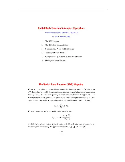
Computing the Output Weights Our equations for the weights are most conveniently written in matrix form by defining matrices with components (Wkj = wkj, (Φpj = φj(xp, and (Tpk = {tkp}. This gives Φ T ΦW T − T = 0 and the formal solution for the weights is ( W T = Φ †T in which we have the standard pseudo inverse of Φ Φ † ≡ (Φ T Φ −1 Φ T which can be seen to have the property Φ †Φ = I. We see that the network weights can be computed by fast linear matrix inversion techniques. In practice we tend to use singular value decomposition (SVD to avoid possible ill-conditioning of Φ , i.e. ΦTΦ being singular or near singular. L13-11Overview and Reading 1. 2. 3. 4. 5. We began by defining Radial Basis Function (RBF mappings and the corresponding network architecture. Then we considered the computational power of RBF networks. We then saw how the two layers of network weights were rather different and different techniques were appropriate for training each of them. We first looked at several unsupervised techniques for carrying out the first stage, namely optimizing the basis functions. We then saw how the second stage, determining the output weights, could be performed by fast linear matrix inversion techniques. Reading 1. 2. Bishop: Sections 5.2, 5.3, 5.9, 5.10, 3.4 Haykin: Sections 5.4, 5.9, 5.10, 5.13 L13-12。