Vnodes An Architecture for Multiple File System Types

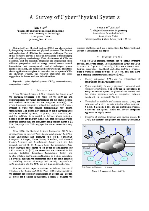
A Survey of Cyber-Physical SystemsJiafu Wan a,ba School of Computer Science and EngineeringSouth China University of Technology,Guangzhou,Chinajiafuwan_76@Hehua Yan*,b,Hui Suo bb College of Information EngineeringGuangdong Jidian PolytechnicGuangzhou,China*Corresponding Author,hehua_yan@Abstract—Cyber Physical Systems(CPSs)are characterized by integrating computation and physical processes.The theories and applications of CPSs face the enormous challenges.The aim of this work is to provide a better understanding of this emerging multi-disciplinary methodology.First,the features of CPSs are described,and the research progresses are summarized from different perspectives such as energy control,secure control, transmission and management,control technique,system resource allocation,and model-based software design.Then three classic applications are given to show that the prospects of CPSs are engaging.Finally,the research challenges and some suggestions for future work are in brief outlined.Keywords-cyber physical systems(CPSs);communications; computation;controlI.I NTRODUCTIONCyber Physical Systems(CPSs)integrate the dynamics of the physical processes with those of the software and communication,providing abstractions and modeling,design, and analysis techniques for the integrated whole[1].The dynamics among computers,networking,and physical systems interact in ways that require fundamentally new design technologies.The technology depends on the multi-disciplines such as embedded systems,computers,communications,etc. and the software is embedded in devices whose principle mission is not computation alone,e.g.cars,medical devices, scientific instruments,and intelligent transportation systems[2]. Now the project for CPSs engages the related researchers very much.Since2006,the National Science Foundation(NSF)has awarded large amounts of funds to a research project for CPSs. Many universities and institutes(e.g.UCB,Vanderbilt, Memphis,Michigan,Notre Dame,Maryland,and General Motors Research and Development Center,etc.)join this research project[3,4].Besides these,the researchers from other countries have started to be aware of significance for CPSs research.In[5-7],the researchers are interested in this domain,including theoretical foundations,design and implementation,real-world applications,as well as education. As a whole,although the researchers have made some progress in modeling,control of energy and security,approach of software design,etc.the CPSs are just in an embryonic stage.The rest of this paper is outlined as follows.Section II introduces the features of CPSs.From different perspectives, the research processes are summarized in Section III.Section IV gives some classic applications.Section V outlines the research challenges and some suggestions for future work and Section VI concludes this paper.II.F EATURES OF CPS SGoals of CPSs research program are to deeply integrate physical and cyber design.The diagrammatic layout for CPSs is shown in Figure1.Obviously,CPSs are different from desktop computing,traditional embedded/real-time systems, today’s wireless sensor network(WSN),etc.and they have some defining characteristics as follows[7-10].∙Closely integrated.CPSs are the integrations of computation and physical processes.∙Cyber capability in every physical component and resource-constrained.The software is embedded inevery embedded system or physical component,andthe system resources such as computing,networkbandwidth,etc.are usually limited.∙Networked at multiple and extreme scales.CPSs,the networks of which include wired/wireless network,WLAN,Bluetooth,GSM,etc.are distributed systems.Moreover,the system scales and device categoriesappear to be highly varied.∙Complex at multiple temporal and spatial scales.In CPSs,the different component has probablyinequable Figure1.Diagrammatic layout for CPSsgranularity of time and spatiality,and CPSs are strictlyconstrained by spatiality and real time.∙Dynamically reorganizing/reconfiguring.CPSs as very complicated systems must have adaptive capabilities.∙High degrees of automation,control loops must close.CPSs are in favor of convenient man-machineinteraction,and the advanced feedback controltechnologies are widely applied to these systems.∙Operation must be dependable,certified in some cases.As a large scale/complicated system,the reliability andsecurity are necessary for CPSs.III.R EASEARCH P ROCESSSince2007,American government has treated CPSs as a new development strategy.Some researchers from various countries discussed the related concepts,technologies, applications and challenges during CPSweek and the international conference on CPS subject[11].The results of this research mainly concentrate in the following respects[7]. A.Energy ControlOne of the features of CPSs is distributed system.Though the vast majority of devices in CPSs need less energy,the energy supply is still a great challenge because the demand and supply of energy is inconvenient.In[12],a control strategy is proposed for realizing best trade-off between satisfying user requests and energy consumption in a data center.In[13-15],these papers concern the basic modeling of cyber-based physical energy systems.A novel cyber-based dynamic model is proposed in which a resulting mathematical model greatly depends on the cyber technologies supporting the physical system.F.M.Zhang et al [16]design optimal and adaptive discharge profile for a square wave impulsive current to achieve maximum battery life.J. Wei et al and C.J.Xue et al[17,18]develop an optimal lazy scheduler to manage services with minimum energy expenditure while not violating time-sensitive constraints.In [19],a peak inlet temperature minimization problem is formulated to improve the energy efficiency.J.R.Cao et al[20] present a clustering architecture in order to obtain good performance in energy efficiency.B.Secure ControlNow,the research for secure control mainly includes key management,identity authentication,etc.In[21],the existing security technologies for CPSs are summarized,and main challenges are proposed.C.Singh et al[22]explore the topic of the reliability assurance of CPSs and possibly stimulate more research in this area.T.T.Gamage et al[23]give a general theory of event compensation as an information flow security enforcement mechanism for CPSs.Then a case study is used to demonstrate this concept.In[24],a certifcateless signature scheme for mobile wireless CPSs is designed and validated.Y.Zhang et al[25]present an adaptive health monitoring and management system model that defines the fault diagnosis quality metrics and supports diagnosis requirement specifications.J.Wei et al[26]exploit message scheduling solutions to improve security quality of wireless networks for mission-critical cyber-physical applications.C.Transmission and ManagementCPSs need to conduct the transmission and management of multi-modal data generated by different sensor devices.In[27], a novel information-centric approach for timely,secure real-time data services in CPSs is proposed.In order to obtain the crucial data for optimal environment abstraction,L.H.Kong et al[28]study the spatio-temporal distribution of CPS nodes.H. Ahmadi et al[29]present an innovative congestion control mechanism for accurate estimation of spatio-temporal phenomena in wireless sensor networks performing monitoring applications.A dissertation on CPSs discusses the design, implementation,and evaluation of systems and algorithms that enable predictable and scalable real-time data services for CPS applications[30].Now,the exiting results are still rare,and there are many facets to be studied.D.Model-based Software DesignNow,the main model-based software design methods include Model Driven Development(MDD)(e.g.UML), Model-Integrated Computing(MIC),Domain-Specific Modeling(DSM),etc[31,32].An example,abstractions in the design flow for DSM,is shown in Figure2.These methods have been widely applied to the embedded system design[34, 35].On the basis of these,some researchers conduct model-based software design for CPSs in the following aspects:event model,physical model,reliability and real-time assurance,etc.Figure2.Abstractions in the design flow for DSM[33]1)Event model.E.A.Lee et al[36]make a case that the time is right to introduce temporal semantics into programming models for CPSs.A programming model called programming temporally-integrated distributed embedded systems(PTIDES) provides a coordination language rooted in discrete-event semantics,supported by a lightweight runtime framework and tools for verifying concurrent software components.In[37],a concept lattice-based event model for CPSs is proposed.This model not only captures the essential information about events in a distributed and heterogeneous environment,but it alsoPlatform mapping Abstractions are linkedthrough refinementrelationsAbstraction layers allowthe verification ofdifferent propertiesPlatform mappingAbstraction layersdefine platformsallows events to be composed across different boundaries of different components and devices within and among both cyber and physical domains.In addition,A CPS architecture along with a novel event model for CPS is developed[38].2)Physical model.In[39],a methodology for automatically abstracting models of CPSs is proposed.The models are described using a user-defined language inspired by assembly code.For mechanical systems,Y.Zhu et al[40]show how analytical models of a particular class of physical systems can be automatically mapped to executable simulation codes.S.Jha et al[41]present a new approach to assist designers by synthesizing the switching logic,given a partial system model, using a combination of fixpoint computation,numerical simulation,and machine learning.This technique quickly generates intuitive system models.3)Reliability and real-time assurance. E. A.Lee[42] emphasizes the importance of security,reliability and real-time assurance in CPSs,and considers the effective orchestration of software and physical processes requires semantic models. From the perspective of soft real-time and hard real-time,U. Kremer[43]conducts the research that the role of time in CPS applications has a fundamental impact on the design and requirements.In CPSs,the heterogeneity causes major challenges for compositional design of large-scale systems including fundamental problems caused by network uncertainties,such as time-varying delay,jitter,data rate limitations,packet loss and others.To address these implementation uncertainties,X.Koutsoukos et al[44]propose a passive control architecture.For improving reliability,T.L. Crenshaw et al[45]describe a simplex reference model to assist developers with CPS architectures which limit fault-propagation.A highly configurable and reusable middleware framework for real-time hybrid testing is provided in[46].Though the model-based software design has an early start, the present development of CPSs progresses at a fast enough rate to provide a competitive challenge.E.Control TechniqueCompared with other control applications,the control technique for CPSs is still at an elementary stage.F.M.Zhang et al[2]develop theoretical results in designing scheduling algorithms for control applications of CPS to achieve balances among robustness,schedulability and power consumption. Moreover,an inverted pendulum as a study object is designed to validate the proposed theory.N.Kottenstette et al[47] describe a general technique:passivity and a particular controller structure involving the resilient power junction.In [48],a design and implementation of CPSs for neutrally controlled artificial legs is proposed.In[49],J.L.Ny et al approach the problem of certifying a digital controller implementation from an input-output,robust control perspective.F.System Resource AllocationUntil now,the relative research for system resource allocation mainly focuses on embedded/real-time systems, networked control systems,WSN,etc[50-52].Towards the complicated CPSs,this work is in the beginning stage.V.Liberatore[53]gives a new train of thought on bandwidth allocation in CPSs.In[54],the model dynamics are presented to express the properties of both software and hardware of CPSs,which is used to do resource allocation.K.W.Li et al [55]research the problem of designing a distributed algorithm for joint optimal congestion control and channel assignment in the multi-radio multi-channel networks for CPSs.The ductility metric is developed to characterize the overload behavior of mixed-criticality CPSs in[56].IV.C LASSIC A PPLICATIONSApplications of CPSs include medical devices and systems, assisted living,traffic control and safety,advanced automotive systems,process control,energy conservation,environmental control avionics and aviation software,instrumentation,critical infrastructure(e.g.power,water),distributed robotics,weapons systems,manufacturing,distributed sensing command and control,smart structures,biosystems,communications systems, etc.[9,10].The classic application architecture of CPSs is described in[38].Now,some application cases for CPSs have been conducted in[57-64].Here,three examples(Health Care and Medicine,Intelligent Road and Unmanned Vehicle,and Electric Power Grid)are used to illuminate the classic applications of CPSs[8,9].A.Health Care and MedicineThe domain of health care and medicine includes national health information network,electronic patient record initiative, home care,operating room,etc.some of which are increasingly controlled by computer systems with hardware and software components,and are real-time systems with safety and timing requirements.A case of CPSs,an operating room,is shown in Figure3.Figure3.A case of CPSs:An operating room[8,9]B.Electric Power GridThe power electronics,power grid,and embedded control software form a CPS,whose design is heavily influenced by fault tolerance,security,decentralized control,and economic/ ethical social aspects[65].In[8,9],a case of CPSs,electric power grid,is given as shown in Figure4.Figure4.A case of CPSs:Electric power grid[8,9]C.Integrate Intelligent Road with Unmanned VehicleWith the development of sensor network,embedded systems,etc.some new solutions can be applied to unmanned vehicle.We are conducting a program that intelligent road and unmanned vehicle are integrated in the form of CPSs.Figure5 shows another case of CPSs:Integrate intelligent road with unmanned vehicle.Figure5.A case of CPSs:Integrate intelligent road with unmanned vehicleV.R ESEARCH C HALLENGESCPSs as a very active research field,a variety of questions need to be solved,at different layers of the architecture and from different aspects of systems design,to trigger and to ease the integration of the physical and cyber worlds[66].In[10, 42,66-68],the research challenges are mainly summarized as follows:1)Control and hybrid systems.A new mathematical theory must merge event-based systems with time-based systems for feedback control.This theory also must be suitable for hierarchies involving asynchronous dynamics at different time scales and geographic scope.2)Sensor and mobile networks.In practical applications, the need for increased system autonomy requires self-organizing/reorganizing mobile networks for CPSs.Gathering and refining critical information from the vast amount of raw data is essential.3)Robustness,reliability,safety,and security.It is a critical challenge because uncertainty in the environment,security attacks,and errors in physical devices make ensuring overall system robustness,security,and safety.Exploiting the physical nature of CPS by leveraging location-based,time-based and tag-based mechanisms is to realize security solutions.4)Abstractions.This aspect includes real-time embedded systems abstractions and computational abstractions,which needs new resource allocation scheme to ensure that fault tolerance,scalability,optimization,etc.are achieved.New distributed real-time computing and real-time group communication methods are needed.In addition,the physical properties also should be captured by programming abstractions.5)Model-based development.Though there several existing model-based development methods,they are far from meeting demands in puting and communications,and physical dynamics must be abstracted and modeled at different levels of scale,locality,and time granularity.6)Verification,validation,and certification.The interaction between formal methods and testing needs to be established. We should apply the heterogeneous nature of CPS models to compositional verification and testing methods.VI.C ONCLUSIONSIn the last few years,this emerging domain for CPSs has been attracting the significant interest,and will continue for the years to come.In spite of rapid evolution,we are still facing new difficulties and severe challenges.In this literature, we concisely review the existing research results that involve energy control,secure control,model-based software design transmission and management,control technique,etc.On this basis,some classic applications used to show the good prospects.Then,we propose several research issues and encourage more insight into this new field.A CKNOWLEDGMENTThe authors would like to thank the National Natural Science Foundation of China(No.50875090,50905063), National863Project(No.2009AA4Z111),Key Science and Technology Program of Guangdong Province(No. 2010B010700015),China Postdoctoral Science Foundation (No.20090460769)and Open Foundation of Guangdong Key Laboratoryof Modern Manufacturing Technology(No. GAMTK201002)for their support in this research.R EFERENCES[1]Available at:/cps/.[2] F.M.Zhang,K.Szwaykowska,W.Wolf,and V.Mooney,“Taskscheduling for control oriented requirements for Cyber-Physical Systems,”in Proc.of2008Real-Time Systems Symposium,2005,pp.47-56.[3]Available at:/news/17248-nsf-funds-cyber-physical-systems-project/.[4]J.Sprinkle,U.Arizona,and S.S.Sastry,“CHESS:Building a Cyber-Physical Agenda on solid foundations,”Presentation Report,Apr2008.[5]Available at:/.[6]Available at:/gdcps.html.[7]J.Z.Li,H.Gao,and B.Yu,“Concepts,features,challenges,andresearch progresses of CPSs,”Development Report of China Computer Science in2009,pp.1-17.[8]R.Rajkumar,“CPS briefing,”Carnegie Mellon University,May2007.[9] B.H.Krogh,“Cyber Physical Systems:the need for new models anddesign paradigms,”Presentation Report,Carnegie Mellon University. [10] B.X.Huang,“Cyber Physical Systems:A survey,”Presentation Report,Jun2008.[11]Available at:/.[12]L.Parolini,N.Toliaz,B.Sinopoli,and B.H.Krogh,“A Cyber-PhysicalSystems approach to energy management in data centers,”in Proc.of First International Conference on Cyber-Physical Systems.April2010, Stockholm,Sweden.[13] F.M.Zhang,Z.W.Shi,and W.Wolf,“A dynamic battery model forco-design in cyber-physical systems,”in Proc.of29th IEEE International Conference on Distributed Computing Systems Workshops.2009.[14]M.D.Ilić,L.Xie,U.A.Khan,et al.“Modeling Future Cyber-PhysicalEnergy Systems,”in Proc.of Power and Energy Society General Meeting-Conversion and Delivery of Electrical Energy in the21st Century,2008.[15]M.D.Ilić,L.Xie,U.A.Khan,et al.“Modeling of future Cyber–Physical Energy Systems for distributed sensing and control,”IEEE Transactions on Systems,Man,and Cybernetics-Part A:Systems and Humans,Vol.40,2010,pp.825-838.[16] F.M.Zhang,and Z.W.Shi,“Optimal and adaptive battery dischargestrategies for Cyber-Physical Systems,”in Proc.of Joint48th IEEE Conference on Decision and Control,and28th Chinese Control Conference,2009,Shanghai,China.[17]W.Jiang,G.Z.Xiong,and X.Y.Ding,“Energy-saving servicescheduling for low-end Cyber-Physical Systems,”in Proc.of The9th International Conference for Young Computer Scientists,2008.[18] C.J.Xue,G.L.Xing,Z.H.Yuan,et al.“Joint sleep scheduling andmode assignment in Wireless Cyber-Physical Systems,”in Proc.of29th IEEE International Conference on Distributed Computing Systems Workshops,2009.[19]Q.H.Tang,S.K.S.Gupta,and G.Varsamopoulos,“Energy-efficientthermal-aware task scheduling for homogeneous high-performance computing data centers:A cyber-physical approach,”IEEE Transactions on Parallel and Distributed Systems,Vol.19,2008,pp.1458-1472. [20]J.R.Cao,and H.A.Li,“Energy-efficient structuralized clustering forsensor-based Cyber Physical Systems,”in Proc.of Symposia and Workshops on Ubiquitous,Autonomic and Trusted Computing,2009. [21] A. A.Cárdenas,S.Amin,and S.Sastry,“Secure control:towardssurvivable Cyber-Physical Systems,”in Proc.of The28th International Conference on Distributed Computing Systems Workshops,2008. [22] C.Singh,and A.Sprintson,“Reliability assurance of Cyber-PhysicalPower Systems,”in Conference Proc.,2010.[23]T.T.Gamage,B.M.McMillin,and T.P.Roth,“Enforcing informationflow security properties in Cyber-Physical Systems:A generalized framework based on compensation,”in Proc.of34th Annual IEEE Computer Software and Applications Conference Workshops,2010. [24]Z.Xu,X.Liu,G.Q.Z,et al.“A cert ificateless signature scheme formobile wireless Cyber-Physical Systems,”in Proc.of The28th International Conference on Distributed Computing Systems Workshops, 2008.[25]Y.Zhang,I.L.Yen,F.B.Bastani,et al.“Optimal adaptive systemhealth monitoring and diagnosis for resource constrained Cyber-Physical Systems,”in Proc.of20th International Symposium on Software Reliability Engineering,2009.[26]W.Jiang,W.H.Guo,and N.Sang,“Periodic real-time messagescheduling for confidentiality-aware Cyber-Physical System in wireless networks,”in Proc.of Fifth International Conference on Frontier of Computer Science and Technology,2010.[27]K.D.Kang,and S.H.Son,“Real-time data services for Cyber PhysicalSystems,”in Proc.of28th International Conference on Distributed Computing Systems Workshops,2008.[28]L.H.Kong,D.W.Jiang,and M.Y.Wu,“Optimizing the spatio-temporal distribution of Cyber-Physical Systems for environment abstraction,”in Proc.of International Conference on Distributed Computing Systems,2010.[29]H.Ahmadi,T.F.Abdelzaher,and I.Gupta,“Congestion control forspatio-temporal data in Cyber-Physical Systems,”in Proc.of the1st ACM/IEEE International Conference on Cyber-Physical Systems,2010.[30]W.Kang,“Adaptive real-time data management for Cyber-PhysicalSystems,”PhD Thesis,University of Virginia,2009.[31]Z.M.Song,“Devlopment method of embedded equipment controlsystems based on Model Integrated Computing,”PhD Thesis,South China University of Technology,2007.[32]Available at:/research/MIC.[33]J.Sztipanovits,“Cyber Physical Systems:New challenges for model-based design,”Presentation Report,Vanderbilt University,Apr2008. [34] F.Li,D.Li,J.F.Wan,et al.“Towards a component-based modelintegration approach for embedded computer control system,”in Proc.of International Conference on Computational Intelligence and Security, 2008.[35] D.Li,F.Li,and X.Huang,et al.“A model based integration frameworkfor computer numerical control system development,”Robotics and Computer-Integrated Manufacturing,Vol.26,2010,pp.848-860. [36] E.A.Lee,S.Matic,S.A.Seshia,et al.“The case for timing-centricdistributed software,”in Proc.of29th IEEE International Conference on Distributed Computing Systems Workshops,2009.[37]Y.Tan,M.C.Vuran,and S.Goddard,“A concept lattice-based eventmodel for Cyber-Physical Systems,”in Proc.of CCPS,Apr2010, Stockholm,Sweden.[38]Y.Tan,M.C.Vuran,and S.Goddard,“Spatio-temporal event model forCyber-Physical Systems,”in Proc.of29th IEEE International Conference on Distributed Computing Systems Workshops,2009. [39]R.A.Thacker,K.R.Jones,C.J.Myers,et al.“Automatic abstractionfor verification of Cyber-Physical Systems,”in Proc.of CCPS,Apr2010, Stockholm,Sweden.[40]Y.Zhu, E.Westbrook,J.Inoue,et al.“Mathematical equations asexecutable models of mechanical systems,”in Proc.of CCPS,Apr2010, Stockholm,Sweden.[41]S.Jha,S.Gulwani,S.A.Seshia,et al.“Synthesizing switching logic forsafety and dwell-time requirements,”in Proc.of CCPS,Apr2010, Stockholm,Sweden.[42] E.A.Lee,“Cyber Physical Systems:Design challenges,”in Proc.ofISORC,May,2008,Orlando,USA.[43]U.Kremer,“Cyber-Physical Systems:A case for soft real-time,”Available at:/.[44]X.Koutsoukos,N.Kottenstette,J.Hall,et al.“Passivity-based controldesign for Cyber-Physical Systems,”Available at:http://citeseerx.ist./.[45]T.L.Crenshaw, E.Gunter, C.L.Robinson,et al.“The simplexreference model:Limiting fault-propagation due to unreliable components in Cyber-Physical System architectures,”in Proc.of IEEE International Real-Time Systems Symposium,2008.[46]T.Tidwell,X.Y.Gao,H.M.Huang,et al.“Towards configurable real-time hybrid structural testing:A Cyber-Physical Systems approach,”in Proc.of IEEE International Symposium on Object/Component/Service-Oriented Real-Time Distributed Computing,2009.[47]N.Kottenstette,G.Karsai,and J.Sztipanovits,“A passivity-basedframework for resilient Cyber Physical Systems,”in Proc.of2nd International Symposium on Resilient Control Systems,2009.[48]H.Huang,Y.Sun,Q.Yang,et al.“Integrating neuromuscular and CyberSystems for neural control of artificial legs,”in Proc.of CCPS,Apr 2010,Stockholm,Sweden.[49]J.L.Ny,and G.J.Pappas,“Robustness analysis for the certification ofdigital controller implementations,”in Proc.of CCPS,Apr2010, Stockholm,Sweden.[50]J.F.Wan,D.Li,and P.Zhang,“Key technology of embedded systemimplementation for software-based CNC system,”Chinese Journal of Mechanical Engineering,Vol.23,2010,pp.241-248.[51]J.F.Wan,D.Li,H.H.Yan,and P.Zhang,“Fuzzy feedback schedulingalgorithm based on central processing unit utilization for a software-based computer numerical control system,”Journal of Engineering Manufacture,Vol.224,2010,pp.1133-1143.[52]J.F.Wan,and D.Li,“Fuzzy feedback scheduling algorithm based onoutput jitter in resource-constrained embedded systems,”In Proc.of International Conference on Challenges in Environmental Science and Computer Engineering,March2010,Wuhan,China.[53]V.Liberatore,“Bandwidth allocation in sense-and-respond systems,”Report,Available at:/~vxl11/NetBots/.[54]M.Lindberg,and K.E.Årzén,“Feedback control of cyber-physicalsystems with multi resource dependencies and model uncertainties,”in Proc.of the31st IEEE Real-Time Systems Symposium,Dec2010. [55]K.W.Li,Q.W.Liu,F.R.Wang,et al.“Joint optimal congestioncontrol and channel assignment for multi-radio multi-channel wireless networks in Cyber-Physical Systems,”in Proc.of Symposia and Workshops on Ubiquitous,Autonomic and Trusted Computing,2009. [56]kshmanan,D.Niz,R.Rajkumar,et al.“Resource allocation indistributed mixed-criticality Cyber-Physical Systems,”in Proc.of International Conference on Distributed Computing Systems,2010. [57] D.Dragomirescu,“Cyber-Physical Systems for aeronautic applications,”Presentation Report,2010,University of Toulouse,France.[58] A.M.K.Cheng,“Cyber-Physical Medical and Medication Systems,”inProc.of the28th International Conference on Distributed Computing Systems Workshops,2008.[59]T.Dillon,and E.Chang,“Cyber-Physical Systems as an embodiment ofdigital ecosystems,”in Proc.of4th IEEE International Conference on Digital Ecosystems and Technologies,2010.[60]J.Madden,B.McMillin,and A.Sinha,“Environmental obfuscation of aCyber Physical System-Vehicle example,”in Proc.of34th Annual IEEE Computer Software and Applications Conference Workshops,2010. [61]I.Lee,and O.Sokolsky,“Medical Cyber Physical Systems,”in Proc.ofDAC,2010,Anaheim,California,USA.[62]W.Harrison,J.Moyne,and D.Tilbury,“Virtual fusion:The completeintegration of simulated and actual,”Presentation Report,2008, University of Michigan,USA.[63]M.Li,Y.H.Liu,J.L.Wang,et al.“Sensor network navigation withoutlocations,”in Proc.of IEEE INFOCOM,2009.[64]G.L.Xing,W.J.Jia,Y.F.Du,et al.“Toward ubiquitous video-basedCyber-Physical Systems,”in Proc.of IEEE International Conference on Systems,Man and Cybernetics,2008.[65] B.McMillin,C.Gill,M.L.Crow,et al,“Cyber-Physical Systemsdistributed control-The advanced electric power grid,”Available at: /.[66]L.Sha,S.Gopalakrishnan,X.Liu,et al.“Cyber-Physical Systems:Anew frontier,”in Proc.of IEEE International Conference on Sensor Networks,Ubiquitous,and Trustworthy Computing,2008.[67]M.Broy,“Cyber-Physical Systems:Technological&scientificchallenges,”Presentation Report,2010.[68]R.Rajkumar,I.Lee,L.Sha,et al.“Cyber-Physical Systems-The nextcomputing revolution,”in Proc.of Design Automation Conference,2010, Anaheim,California,USA.。

Trane VariTrane™ VAVTerminal UnitBreakthrough with VAV technology.VariTrane – leadership redefinedTrane is pleased to introduce a breakthrough in Variable Air Volume (VAV) technology—the new Trane VariTrane™ VAV terminal unit. VariTrane units are manufactured in the most state-of-the-art VAV facility in the world. Proven components, such as the patented Trane Flow Ring and the Trane DDC controller, are used. The most advanced manufacturing techniques in the industry have been implemented to provide an exceptionally rugged and reliable VAV unit. All products are UL® listed for safety and provide proven performance via accepted industrystandards like ARI-880 and plete VAV control offeringAll VariTrane VAV controls are factory commissioned. This means that airflow, temperature setpoints, and addressing are performed in a controlled factory environment. 100% factory-run testing is included to ensure that units arrive and function properly upon job startup. With factory commissioned controls, you have better control over cost and quality. This results in a higher quality installation at a lower cost.23Trane factory-commissioned controls include: • DDC controller, the VAV Unit Control Module (UCM)—Optimized performance and integration to Trane Tracer® systemTrane controller communication p rotocols include: • Trane proprietary (COMM4), LON™ and BACnet™• Wireless options for the zone sensor AND unit to unit communication• Pneumatic controller—Field configurable for reverse- or direct acting thermostatsFactory-installation of customer furnished controls:Some customers prefer to provide their own controller to be installed in our manufacturing facility. In these cases, Trane will:• Ensure compatibility with unit relays, fuses, a nd transformer• Install the controller, including piping the pressure transducer to the Trane flow ring• Coordinate with the owner’s preferred control vendorThe factory-installed controller option has been availablesince the early 1990s. It provides unlimited controller flexibility for building owners, and should be considered when Trane controls are not required.Take a look inside the VariTrane™ unit.All VariTrane units have the following:• Trane flow ring for unmatched airflowmeasurement accuracy• Heavy gage air valve cylinder• Interlocking panels which create an e xtremelyrugged unit• Insulation edges are encapsulated w ith metal• UL® and CUL® listing• Fusing and disconnects (optional)• Control power transformers (optional)Single-duct and dual-duct air terminals:• Single-duct reheat options include w ater orelectric-heating coils• Unit sizes provide 0 to 8000 nominal cfm• Access for water coil cleaning• Factory-commissioned Trane controls• Factory installation of customer s uppliedcontrollers• Slip and Drive connections as standardFan-powered air terminals:• Parallel intermittent fan and series c ontinuousfan configurations• Complete reheat options include water o relectric-heating coils• Fan sizes provide 200 to 3000 nominal cfm• Single-speed motor with SCR is standard f or simplified system balancing• Optional high efficiency ECM motors• Low-height models for critical plenumrequirementsABCDE4F G BCDEFGControls – Trane installsmore customer- supplied VAVcontrollers than any othermanufacturer in the industry. Forthe highest quality and reliability,demand Trane controls.Flow Ring – The patented Traneflow ring provides unmatchedairflow measurement accuracyand unit performance. It isrecessed within the 18-gageair valve cylinder for protectionduring jobsite handling andinstallation.External Shaft – Comes with AirValve Position Indicator for easierservice diagnostics. An externalshaft also simplifies mounting ofall brands of controllers.Fan Controls – Now comes witha standard SCR or ElectricallyCommutated Motors (ECM) usedfor fan-speed control and systembalancing.Air Valve – Designed to limitinlet deformation and provideconsistent and repeatable airflowacross the flow ring.Interlocking Panels –Ruggedness and rigidity areassured with Trane’s patentpending interlocking panelconstruction. I t createsunmatched unit rigidity.Metal Encapsulated Edges – AllVariTrane Units are complete withencapsulated edges to arrest cutfibers and prevent erosion in theairstream. This raises the b ar inthe VAV industry.5Trane Air-Fi Wireless SystemsWhen using one of the Trane BACnet™ control platforms, optionally the VAV terminal units can be configured from the factory with Trane Air-Fi Wireless technology. This option eliminates the need for, and expense of, a wired communication link between units. It provides wireless unit to zone sensor communication and wireless unit to unit communication.Fail-Safe DesignAir-Fi utilizes a mesh network. This flexible, resilient system architecture has built-in redundancy to protect against interference and outages. The network automatically re-routes signals around obstacles; it bypasses damaged nodes. The dynamic adaptability of the network ensures reliable communication.Wide Range CoverageEach device has four times the number of potential paths out to the network. The 200-foot indoor signal range can extend to half a mile when unobstructed. With multiple paths and a long-range signal, Trane Air-Fi devicescan be linked together to create strong, stable, blanket coverage across an entire site.Performance: Part of the PackageThe Trane Air-Fi interface is available as a factory-installed option. It includes a lifetime battery* to deliver a maintenance-free power supply over the life of the system.*Based on typical indoor operating conditions. All about Trane Air-Fi™ Wireless Systems.Visit /AirFi for more information onTrane Air-Fi Wireless Systems.67Energy efficiencyAsignificant consumer of energy in commercial buildings is heating and air conditioning. One of the most energy-efficient HVAC solutions is the VAV system.This has led to a steady increase in VAV systems over the past several years. VAV systems save significant energy, comply with ventilation requirements, and provide reliable and personalized occupant comfort.Energy-saving features of Trane VAV terminal units include:• System strategies like Ventilation Reset,and Static Pressure Optimization, etc. • Night setback• Occupied/unoccupied control • Demand controlled ventilation • Electrically Commutated Motors (ECM)• EarthWise™ Systems utilizing low temperature air To determine the potential energy savings a VAV system can bring to your applications, Trane offers energy modeling programs like System Analyzer™, a nd TRACE 700™ simulation software.Doesn’t ICS increase VAV system complexity, which may impact reliability?Not really. Again, most VAV systems are alreadyusing communicating controllers on VAV units and air handlers. Control strategies that save energy are pre-programmed into the VAV controller and Trane Tracer™Complete systemsinclude VariTrane™ units.System, which eliminates field programming errors and complexities. Implementing them only requires minimal time and it actually improves system reliability! All Trane VAV controllers are factory commissioned. This means that all temperature and airflow setpoints are downloaded and 100% run tested in the factory before shipment. You can be assured that Trane DDC systems are the most reliable system available!SummaryAn integrated system is essential for complete building environmental comfort and system efficiency. Through the use of factory-commissioned controllers, and the existing capabilities of the DDC system, additional energy saving strategies can be implemented. At the same time, the system maintains the highest reliability in the industry. Call your local Trane Sales Office for additional details.% H V A C E n e r g y C o n s u m p t i o nMiamiMinneapolisTorontoSeattle System 1Analysis performed with TRACE® 700 building energy and economic analysis software.System 1with pressure optimizationSystem 1with ventilation reset and pressure optimizationIntegrated Comfort™ Systems (ICS)Trane Integrated Comfort™ Systems (ICS) combines VariTrane VAV terminal units, Trane DDC controls, and factory commissioning. Trane ICS enables system-level control strategies like Ventilation Reset and Static Pressure Optimization to improve system performance and efficiency. It’s like fuel injection in a car’s engine. A gravity-fed carburetor will provide gas to your car’s engine, but fuel injection does it in the most efficient manner, while boosting horsepower. ICS is just that—ahorsepower and efficiency boost for your VAV system!Learn more at Trane – by Trane Technologies (NYSE: TT), a global climate innovator – creates comfortable, energy efficient indoor environments through a broad portfolio of heating, ventilating and air conditioning systems and controls, services, parts and supply. For more information, please visit or .© 2020 Trane. All Rights Reserved. All trademarks referenced in this document are the trademarks of their respective owners.VAV-SLB004-EN06/02/2020。

A Guide to Elasticsearch SnapshotsThis article originally appeared on and is republished with permission from the author.As Elasticsearch matures, it is no longer just used to power search boxes. Instead, Elasticsearch is now moving to the core of data-powered systems. Business-critical databases require a serious data protection strategy. This post focuses on how to set up and use snapshots for Elasticsearch clusters running in Kubernetes.This post builds upon a previous post that covers how to set up either an S3 or NFS snapshot repository in Elastic Cloud Enterprise and FlashBlade’s snapshot/restore performance. I will focus here on how to back up Elasticsearch clusters running using Elastic Cloud for Kubernetes (ECK).What you should learn from this blog:How to configure a snapshot repository on an on-premises S3 object storeHow to set up and use a shared filesystem repository on NFS using a dynamically provisioned ReadWriteMany PersistentVolumeT e c h n i q u e s t o s i m p l i f y s e t t i n g u p a n d u s i n g Elasticsearch snapshots in KubernetesSnapshot repositories enable powerful data protection workflows: recovering from user error and accidental deletion, restoration after infrastructure outages, and finally, cloning indices for dev/test workflows. And because the repositories can be shared amongst disparate clusters, you can restore and share indices across internal and public clouds.An example possible topology is illustrated below with twodistinct Kubernetes clusters, likely in different availability zones. Each cluster uses a local FlashBlade® as primary storage for Elasticsearch clusters, where latency is important, and the other FlashBlade as a primary snapshot repository. As you can see in the diagram, the Elasticsearch cluster in site 2 can restore from the local repository, enabling you to recover indices in a different site if needed. Not shown here is a similar connection from both clusters to the snapshot repository on FlashBlade A.Figure 1: A possible DR architecture for multiple Kubernetes clusters. Site 2 can also use FlashBlade A as a snapshotrepository.With high performance, all-flash storage like FlashBlade, the snapshot and restores consistently achieve multiple GB/s throughput. With this performance, the bottleneck often moves to the Elasticsearch nodes themselves and not the snapshot repository. Storing snapshot repositories on FlashBlade complements the ability to run primary storage for Elasticsearch on PersistentVolumes provided by FlashBlade. As a bonus, when using FlashBlade for the snapshot repository (either S3 or NFS), my use case gets a 40% space reduction dueto inline compression.S3 Snapshot RepositoryFor an S3 snapshot repository, I programmatically install the necessary plugin on all Elastic nodes using init-containers. This is simpler than the alternative approach of building a custom image with the plugin included.Add the initContainer spec to your Elasticsearch cluster definition (yaml) for the ECK operator:initContainers:- name: install-pluginscommand:- sh- -c- |bin/elasticsearch-plugin remove --batch repository-s3bin/elasticsearch-plugin install --batch repository-s3The plugin is first removed to avoid subsequent failure to install if the plugin already exists.By default, ECK enforces security in Elasticsearch clusters. As a result, we need to take care in providing our S3 access keys via a second init-container. I use a technique inspired by this blog, injecting the keys as environment variables and piping them into the Elasticsearch keystore.The full pair of initContainers, named “install-plugins” and “add-access-keys,” looks as follows:initContainers:- name: install-pluginscommand:- sh- -c- |bin/elasticsearch-plugin remove repository-s3bin/elasticsearch-plugin install --batch repository-s3 - name: add-access-keysenv:- name: AWS_ACCESS_KEY_IDvalueFrom:secretKeyRef:name: irp210-s3-keyskey: access-key- name: AWS_SECRET_ACCESS_KEYvalueFrom:secretKeyRef:name: irp210-s3-keys <c/ode>key: secret-keycommand:- sh- -c- |echo $AWS_ACCESS_KEY_ID | bin/elasticsearch-keystore add --stdin --force s3.client.default.access_keyecho $AWS_SECRET_ACCESS_KEY | bin/elasticsearch-keystore add --stdin --force s3.client.default.secret_keyThis technique relies upon the access keys being created as secrets with a one-off process, ideally immediately after the keys are created on the FlashBlade.> kubectl create secret generic my-s3-keys --from-=’XXXXXXX’ --from-literal=secret-=access-keyliteralkey=’YYYYYYY’By default, Elasticsearch’s snapshot operations are limited to a single thread, which limits maximum possible performance. The maximum size of the thread_pool can be modified on each n o d e a t s t a r t u p t i m e o n l y t h r o u g h a p a r a m e t e r i n elasticsearch.yaml. For the ECK operator, add this parameter to the “config” section of each nodeSet:config:node.master: truenode.data: truenode.ingest: truethread_pool.snapshot.max: 8You can now create a snapshot repository with the following example json configuration.{“type”: “s3”,“settings”: {“bucket”: “elastic-snapshots”,“endpoint”: “10.62.64.200”,“protocol”: “http”,“max_restore_bytes_per_sec”: “1gb”,“max_snapshot_bytes_per_sec”: “200mb”}}Replace the endpoint field with a data VIP for your FlashBlade and ensure that the destination bucket has been created already. The bucket can be created through the FlashBlade UI, CLI, or REST API.The command guide in a later section will demonstrate the specific command to use curl to create the repository.NFS Snapshot RepositoryWe can also use a shared filesystem snapshot repository as a backend to store snapshots on NFS without requiring any additional plugin installation. This is useful if a performant S3 object store is not available.T o c r e a t e a s h a r e d f i l e s y s t e m w i t h N F S,I m o u n t a ReadWriteMany (RWX) PersistentVolume on all of the Elasticsearch nodes. This volume is backed by an NFS filesystem automatically provisioned by my Pure Service Orchestrator™ plugin. I could use a statically provisioned filesystem also, which would allow connections from other clusters.Create a PersistentVolumeClaim (PVC) in ReadWriteMany mode:kind: PersistentVolumeClaimapiVersion: v1metadata:name: es-snap-repo-claimspec:storageClassName: pure-fileaccessModes:- ReadWriteManyresources:requests:storage: 10TiThis PVC assumes the ‘pure-file’ storageClass is installed and configured via PSO for FlashBlade connectivity. Otherwise, you will need to use the appropriate storageClass.Then, simply add this volume as a mount to the pod template in your elasticsearch.yaml definition:nodeSets:- name: all-nodescount: 5podTemplate:spec:containers:- name: elasticsearchvolumeMounts:- name: es-snap-repo-volmountPath: /es-snaps…volumes:- name: es-snap-repo-volpersistentVolumeClaim:claimName: es-snap-repo-claimWe also need to set path.repo to this mounted path in the yaml file for the Elasticsearch cluster:config:node.master: truenode.data: truenode.ingest: truethread_pool.snapshot.max: 8path.repo: [“/es-snaps”]Once the cluster is configured and running, a shared filesystem snapshot repository is created. The JSON of its configuration is:{“type”: “fs”,“settings”: {“location”: “/es-snaps”,“compress”: false,“max_restore_bytes_per_sec”: “1gb”,“max_snapshot_bytes_per_sec”: “1gb”}}Since both S3 or NFS work as snapshot repositories, it is important to understand the trade-offs when choosing which to use. You will have noticed subtle differences in installation and configuration of the repository, but the biggest factor that favors S3 is the storage lifetime. A snapshot repository on S3 is not tied to a single Kubernetes cluster as with a dynamically provisioned PersistentVolume. As a result, you can snapshot and restore between entirely different Kubernetes clusters. But you can also achieve the same portability with statically provisioned NFS volumes. My recommendation is to prefer S3 if available.Snapshot Command GuideAdministering an Elasticsearch cluster means using the REST API as a primary tool for interaction, especially if you want to build automation around your usage. The ubiquitous command line tool curl is a versatile client for any REST API and one I use heavily with Elasticsearch.Instead of always manually crafting curl commands as needed, I find it very useful to create a workflow that lets me repeat similar tasks more quickly. The first step for that is an environment to run the curl commands and second is a catalog of pre-built commands that can be copy-pasted, reused, and modified easily.The jump host is a plain pod: a simple container image with curl installed by default. To simplify further commands, I create two important environment variables that simplify connecting to a specific cluster. The first pulls in theElasticsearch cluster’s password and the second encodes the cluster’s service name. If I have two different Elasticsearch clusters, I can simply make two versions of this pod and use the same exact command strings.apiVersion: v1kind: Podmetadata:name: es-jumpspec:containers:- name: es-jumpimage: centos:7env:- name: PASSWORDvalueFrom:secretKeyRef:name: quickstart-es-elastic-userkey: elastic- name: ESHOSTvalue: “https://quickstart-es-http:9200"command: [“tail”, “-f”, “/dev/null”]imagePullPolicy: IfNotPresentrestartPolicy: AlwaysLog in to this jump pod using ‘kubectl exec’ to create a new bash prompt:> kubectl exec -it pod/es-jump bashAlternatively, you could manually define the environment variables in any shell that has access to the Elasticsearch cluster. The jump pod is my personal preference.Quick ES Snapshot Command Cheat SheetThis cheat sheet is an adaptation of the Elastic API documentation and contains useful commands for manually taking and managing snapshots.First, perform basic health checks and view indices:curl -u “elastic:$PASSWORD” -k “$ESHOST/_cat/health?v”curl -u “elastic:$PASSWORD” -k “$ESHOST/_cat/nodes?v”curl -u “elastic:$PASSWORD” -k “$ESHOST/_cat/indices?v”List snapshot repositories:curl -u “elastic:$PASSWORD” -k “$ESHOST/_snapshot?pretty”Create a snapshot repository named “my_s3_repository”:c u r l-u“e l a s t i c:$P A S S W O R D”-k-X P U T “$ESHOST/_snapshot/my_s3_repository?pretty” -H ‘Content-Type: application/json’ -d’{“type”: “s3”,“settings”: {“bucket”: “elastic-snapshots”,“endpoint”: “10.62.64.200”,“protocol”: “http”,“max_restore_bytes_per_sec”: “1gb”,“max_snapshot_bytes_per_sec”: “200mb”}}‘Delete a snapshot repository:c u r l-X D E L E T E-u“e l a s t i c:$P A S S W O R D”-k “$ESHOST/_snapshot/my_s3_repository?pretty”Note that if you delete a repository and then recreate it with the same storage backend, the previously taken snapshots are still available.In other words, deleting a snapshot repository definition does not delete the snapshots.List snapshots in a repository:c u r l-u“e l a s t i c:$P A S S W O R D”-k “$ESHOST/_cat/snapshots/my_s3_repository?v”Start a snapshot of all indices and give the snapshot a date-based name:c u r l-u“e l a s t i c:$P A S S W O R D”-k-X P U T $ESHOST/_snapshot/my_s3_repository/test-snapshot-$(date +”%Y-%m-%d-%H-%M”)?prettyTake a snapshot and wait for completion before returning:c u r l-u“e l a s t i c:$P A S S W O R D”-k-X P U T $ESHOST/_snapshot/my_s3_repository/test-snapshot-$(date +”%Y-%m-%d-%H-%M”)?wait_for_completion=true&prettyTake a snapshot of one specific index:c u r l-u“e l a s t i c:$P A S S W O R D”-k-X P U T $E S H O S T/_s n a p s h o t/m y_s3_r e p o s i t o r y/t e s t-snapshot?wait_for_completion=true -H ‘Content-Type: application/json’ -d’{ “indices”: “nyc_taxis” }’List info about a specific snapshot:c u r l-u“e l a s t i c:$P A S S W O R D”-k “$E S H O S T/_s n a p s h o t/m y_s3_r e p o s i t o r y/t e s t-snapshot/_status?pretty”Delete a snapshot:c u r l-X D E L E T E-u“e l a s t i c:$P A S S W O R D”-k “$ESHOST/_snapshot/my_s3_repository/test-snapshot?pretty”Restore from snapshot into a new index:c u r l-u“e l a s t i c:$P A S S W O R D”-k-X P O S T $E S H O S T/_s n a p s h o t/m y_s3_r e p o s i t o r y/t e s t-snapshot/_restore?pretty -H ‘Content-Type: application/json’ -d’{ “indices”: “nyc_taxis”, “rename_pattern”: “nyc_taxis”,“rename_replacement”: “restored_taxis” }’For testing snapshot recovery, it is often useful to delete an index “accidentally”:c u r l-X D E L E T E-u“e l a s t i c:$P A S S W O R D”-k “$ESHOST/restored_taxis?pretty”Recall that one of the recommendations for snapshot and restore performance was to increase the size of the threadpool at startup time. Confirm these threadpool settings:c u r l-u“e l a s t i c:$P A S S W O R D”-k “$ESHOST/_cat/thread_pool/snapshot?h=name,max&v”When using a shared filesystem repository, the REST API is exactly the same, just specify a different repository name.Take snapshot with my NFS repository:c u r l-u“e l a s t i c:$P A S S W O R D”-k-X P U T $ESHOST/_snapshot/my_nfs_repository/test-snapshot?prettyList snapshots in NFS repository:c u r l-u“e l a s t i c:$P A S S W O R D”-k “$ESHOST/_cat/snapshots/my_nfs_repository?v”Restore from snapshot in an NFS repository:c u r l-u“e l a s t i c:$P A S S W O R D”-k-X P O S T $E S H O S T/_s n a p s h o t/m y_n f s_r e p o s i t o r y/t e s t-snapshot/_restore?pretty -H ‘Content-Type: application/json’ -d’{ “indices”: “nyc_taxis”, “rename_pattern”: “nyc_taxis”,“rename_replacement”: “restored_taxis” }’Snapshot Lifecycle ManagementElasticsearch includes a module, Snapshot Lifecycle Management (SLM), that automates snapshot scheduling and allows you to keep snapshots for a specified amount of time. For newer releases of Elasticsearch (7.4+) that include SLM, this module nicely solves the majority of snapshot use cases.Verify that SLM is running:curl -u “elastic:$PASSWORD” -k “$ESHOST/_slm/status?pretty”View existing snapshot policies:curl -u “elastic:$PASSWORD” -k “$ESHOST/_slm/policy?pretty”Create a snapshot policy named ‘daily-snapshots’ that applies to a subset of indices:c u r l-X P U T-u“e l a s t i c:$P A S S W O R D”-k “$ESHOST/_slm/policy/daily-snapshots?pretty” -H ‘Content-Type: application/json’ -d’{“schedule”: “0 30 1 * * ?”,“name”: “<daily-snap-{now/d}>”,“repository”: “my_s3_repository”,“config”: {“indices”: [“plsidx-*”, “nyc_taxis”],“ignore_unavailable”: true,“include_global_state”: false},“retention”: {“expire_after”: “30d”,“min_count”: 5,“max_count”: 50}}‘For more information about snapshot policy options, see the Elastic documentation.Check statistics for snapshot and retention operations:curl -u “elastic:$PASSWORD” -k “$ESHOST/_slm/stats?pretty”Finally, delete a snapshot policy as follows:c u r l-X D E L E T E-u“e l a s t i c:$P A S S W O R D”-k “$ESHOST/_slm/policy/daily-snapshots?pretty”Custom Kubernetes CronJobThere will be occasions when SLM does not have the flexibility to do exactly what you need. In those cases, you can manually trigger snapshots with automation like Kubernetes jobs or CronJobs.One example would be a daily job that pulls audit logs from network devices and sends that data to Elasticsearch. Using a technique like below, you can also automate taking a snapshot immediately after the index has been finished. And perhaps this could be used to make searchable snapshots available once that feature arrives…An easy way to automate the creation of snapshots utilizes Kubernetes CronJobs. Full yaml for a snapshot CronJob follows:apiVersion: batch/v1beta1kind: CronJobmetadata:name: elasticsearch-snapshotterspec:schedule: “@daily”concurrencyPolicy: ForbidjobTemplate:spec:template:spec:containers:- name: snapshotterimage: centos:7env:- name: ESPASSWORDvalueFrom:secretKeyRef:name: quickstart-es-elastic-userkey: elasticcommand:- /bin/bashargs:- -c- |curl -s -i -k -u “elastic:$ESPASSWORD” -XPUT “https://quickstart-es-http:9200/_snapshot/my_s3_repository/%3 Csnapshot-%7Bnow%2Fd%7D%3E" | tee /dev/stderr | grep “200 OK”restartPolicy: OnFailureCombine snapshots with more customized workflows using this simple curl invocation as a building block with no complicated dependencies or configuration required.SummaryElasticsearch is more and more a crucial underpinning of data platforms; the need for a data protection strategy arises. Fortunately, configuring and using snapshot repositories is straightforward and flexible. FlashBlade as a data platforms e r v e s a s b o t h t h e p e r f o r m a n t p r i m a r y s t o r a g e f o r Elasticsearch clusters and simultaneously as a snapshot repository for backups and fast restores.。

UTRAN LONG TERM EVOLUTION IN 3GPPAntti Toskala Harri Holma Kari Pajukoski Esa Tiirola Nokia Networks Nokia Networks Nokia Networks Nokia Networks P.O. Box 301 P.O. Box 301 P.O.Box 319 P.O.Box 31900045 NOKIA GROUPFinland 00045 NOKIA GROUPFinland90651 OULUFINLAND90651 OULUFINLANDA BSTRACTThe 3rd Generation Partner Ship Project (3GPP) produced the first version of WCDMA standard in the end of 1999, which is the basis of the Universal Mobile Telephone System (UMTS) deployed in the field today. This release, called release 99, contained all the basic elements to meet the requirements for IMT-2000 technologies. Release 5 introduced the High Speed Downlink Packet Access (HSDPA) in 2002, enabling now more realistic 2 Mbps and even beyond with data rates up to 14 Mbps. Further Release 6 followed with High Speed Uplink Packet Access (HSUPA) in end of 2004, with market introduction expected in 2007. Alongside with on-going further WCDMA development, work on Evolved Universal Terrestrial Radio Access (UTRA) has been initiated in 3GPP. The objective of Evolved UTRA is to develop a framework for the evolution of the 3GPP radio-access technology towards wider bandwidth, lower latency and packet-optimized radio-access technology with peak data rate capability up to 100 Mbps. This paper introduces the requirements, the current state of progress in 3GPP, findings on the performance, agreed architecture as well as expected schedule for actual specification availability.1.INTRODUCTIONFollowing the first wave of WCDMA based networks rollout with data rates up to 384 kbps both in the uplink and downlink [1], now the High Speed Downlink Packet Access (HSDPA) is being rolled out with 2-3 Mbps practical data rate capabilities and theoretical peak rate of 10 Mbps or even more and with High Speed Uplink Packet (HSUPA) set to follow during 2007 with capability up to 5.7 Mbps in the uplink as well [2].In order to prepare for future needs, 3GPP has initiated activity on the long term evolution of UTRAN (Universal Terrestrial Radio Access Network), which is aiming clearly beyond to what the WCDMA can do with HSDPA or HSUPA in case of uplink. The UTRAN long-term evolution work is looking for the market introduction of Evolved UTRAN (EUTRAN) around 2010, with resulting specification availability planned toward end of 2007. The feasibility study is currently on going and key decisions on the multiple access as well as on the protocol architecture have been recently reached. Feasibility study finalization is expected for September 2006 time frame, after which actual specification development would start. This paper covers in section 2 the requirements for the work defined in 3GPP, and then looks at the network and protocol architecture developments in section 3. Section 4 covers the physical layer technology selection. Section 5 addressed the feasibility study findings on the performance and remaining work and expected schedule is covered in section 6. Conclusions are drawn in section 7.2.REQUIREMENTSFor the long term evolution, clearly more ambitious goals were necessary to make it worth the effort compared with what can be achieved with current system. Thus the following targets were defined [3]:•User plane latency below 5 ms with 5 MHz or higher spectrum allocation. With spectrum allocationbelow, latency below 10 ms should be facilitated.•Reduced control plane latency•Scalable bandwidth up to 20 MHz, with smaller bandwidths covering 1.25 MHz, 2.5 MHz, 5 MHz,10 MHz and 15 MHz for narrow allocations. Also1.6 MHz is considered for specific cases.•Downlink peak data rates up to 100 Mbps•Uplink peak data rates up to 50 Mbps• 2 to 3 times capacity over the existing Release 6 reference scenarios with HSUPA• 2 to 4 times capacity over the existing Release 6 reference scenarios with HSDPA•Improved end user data rates at the cell edge•Support for packet switched (PS) domain onlyWhile big investments have been done and are being done in WCDMA and GSM based networks, also inter-working with WCDMA and GSM is a key requirement for a new system part of the 3GPP technology family. The requirement for handover between legacy systems and E-UTRAN is for services with real time quality a break of 300 ms and for the non-real time services 500 ms would be sufficient.Further there is a desire to have reduced operating cost (often referred as OPEX) and reduced network investment costs (often referred as CAPEX).The agreed baseline assumptions also include 2 receiver antennas in the mobile terminal, which facilitates usage of advanced antenna technologies, such as Multiple Input Multiple Output (MIMO) antenna concepts. Respectively, a typical base station is expected to have two antennas transmit and receive capabilities.The defined mobility support are aiming for optimized performance for mobile speed of less than 15km/h, and high performance for speeds up to 120km/h, and the connection should be maintained with mobile speeds even up to 350 km/h.1-4244-0330-8/06/$20.00 2006 IEEEWORK ARCHITECTUREThe long-term evolution network architecture is characterised by three special requirements:•Support for PS domain only i.e. there will not be connection to circuit switched (CS) domain nodes,such as the Mobile Switching Centre, but speechservices need to be handled as Voice over IP (VoIP)calls.•Tight delay targets for small roundtrip delay. The roundtrip delay target is 5 ms for bandwidths of 5MHz or more. Respective target is 10 ms for thebandwidths of below 5 MHz.•Reduced cost of the systemThe architecture proposals made for the study could be characterized under two categories:•BTS based approach, which adds more functionality for the base station and having all radio relatedfunctionalities in the BTS•Two node architecture for radio protocols with radio related signalling etc. terminating in the node abovebase station.Following the intensive discussion, it was agreed to use two node architecture, with the functionality divided between two network elements, eNode B and access gateway (aGW). Itwas then agreed that radio related signalling (RRC) as well as all layers of retransmission are located in eNode B. MAC layer functionality etc, similar to HSDPA/HSUPA operation, will remain in the eNode B as well. Ciphering and header compressions were decided to be located in aGW, as shown in Fig. 1. The interface connecting aGW and eNode B (BTS) is called S1 interface and that will have some similarity with the Iu interface between the current radio access network and core network, though the functional split is slightly different due to the ciphering and header compression in core network (aGW) side. Further interface called X2 will be defined between eNode Bs for e.g. handover purposes.One of the key issues impacting the architecture was the potential need and type of macro diversity combining to be supported for EUTRAN. As with was decided that there no need for macro-diversity, similar combining functionality as with WCDMA in Radio Network Controller (RNC) [2] was not needed.server for future study.IV.MULTIPLE ACCESS TECHNOLOGY Following the requirements laid down for the multiple access technologies, it has become evident that something else than the use of the current radio interface technology needs to be considered for the radio access supporting up to 100 Mbps and up to 20 MHz bandwidth. While the WCDMA radio interface technology, as described in details in [1], is very efficient for proving (downlink peak) data rates up to 10 Mbps, the requirements such as reaching 100 Mbps peak rate rates cannot be met with WCDMA technology with reasonable mobile terminal complexity. As an example in the downlink direction this would require either multiple 5 MHz carriers or higher chip rate, neither of the solutions very attractive when aiming for very high performance with advanced receivers in the mobile terminal.As this was clearly understood in 3GPP community, the decision was made to adopt the for the uplink direction the Single Carrier FDMA (SC-FDMA) due to the good performance in general and superior properties in terms of uplink signal Peak-to-Average Ratio (PAR) when compared to OFDM in the uplink. In the downlink direction the solution was OFDM, mainly due to the simplicity of the terminal receiver in case of large bandwidths in difficult environment. Also for the network side transmission PAR was not considered such a key problem.The following sub-sections on multiple access details focus on operation with the paired frequency bands (by using frequency division duplex, FDD), though work in 3GPP covers also time division duplex (TDD).A. DownlinkFor downlink, the adoption of OFDMA enabled flexiblesupport of different bandwidth options. The basic OFDMchain is illustrated in Fig. 2 as used for the feasibility studiesat least, though obviously several advanced techniques arebeing considered on top of the basic OFDMA operation.These technologies include frequency domain scheduling,MIMO antenna technologies and variable coding andOne of the key aspects for the air interface is a scalablesolution to support the large number of different bandwidths,starting from 1.25 MHz and all the way to 20 MHz. Thesingle set of parameters for sub-carrier spacing etc. providesupport for different bandwidths by only changing the numberof sub-carriers while keeping the frame length as well assymbol length constant. The parameters defined during thefeasibility study can be found from [6].B. UplinkThe chosen SC-FDMA solutions are based on the use ofcyclic prefix to allow for high performance and lowcomplexity receiver implementation in the base station. Thereare two different variants of SC-FDMA under discussion,which differ from each other only from the spectrum use. Theso called blocked or localized FDMA uses a continuesfrequency band for a single users while with the InterleavedFDMA (IFDMA) the frequency band is used in non-continuous way, as described for example in [3], but only stilltransmitting one modulation symbol in time domain; thusretaining the advantage of low PAR (sometimes referred as crest factor) when compared to OFDMA. With FDMA the type of modulation applied will impact the PAR, but with OFDMA the large number of parallel sub-carriersFigure 3: FDMA and IFDMA principles for frequencydomain generation of signals.make the resulting PAR 2-6 dB higher than FDMA. 3GPP did decide in December 2005 to use FDMA for PAR reasons. The conceptual transmission methods of localized FDMA and IFDMA are illustrated in Fig. 3. OFDM is well know from e.g. the IEEE 802.11 standardsfamily, while FDMA variants with cyclic prefix representnewer proposals for wireless mobile communicationstandards, though it has been published for almost a decadeago, for example in [4].For the uplink considerations the cell edge operation ishighlighted due operator requirements. A mobile data servicethat provides a high data rates in the majority of the cell areais easier to market and sell compared to a mobile data servicethat severely limits the high data rate availability to a smallfraction of the cell area. Hence even a few dBs improvementin PAR is very essential to achieve high data rate availabilityclose to cell edge.The general FDMA transmitter and receiver concept (notdirectly usable for IFDMA) is illustrated in Fig. 4. With thegeneration of IFDMA the block repetition after modulatorshould added or other alternative is the use of FFT/IFFT inthe transmitter as well. Those could be applied to produce theFDMA signal as well, as seen in the example in Fig. 3 withboth IFDMA and FDMA principles illustrated. In case ofIFDMA multiple users can then share the frequency domainresource by using different offset for starting their sub-carrieroccupancy. IFDMA is more sensitive to imperfections likefrequency offset as there are now more borders between usersin frequency domain.In 3GPP discussions an important learning was also that oneshould use instead of PAR, so called Cubic Metric [5] insteadfor describing the impact for the power amplifiers due tosignal envelope variations. The use of CM takes better thepractical amplifier properties into account compared to PAR.The OFDMA and SC-FDMA uplink CM comparison isshown in Fig. 5, indicating the difference depending on themodulation being used. With optimised modulation thedifference may be up to 4 dB in the favour of SC-FDMA.FDMAIFDMATransmitterdomain signal generation.C. Physical layer parameter selectionThe work is on-going to identify the base parameters, such as the transmission time interval (TTI) to be used. For the feasibility study a common parameter set has been agreed, with the example shown in Table 1 for 5 and 10 MHz bandwidths. The common nominator for all bandwidths is theshort TTI of 0.5 ms; this was chosen to enable a very short latency with L1 Hybrid ARQ as already introduced with HSDPA and HSUPA [2].Table 1: Downlink Parameters for 5 and 10 MHz bandwidths. Bandwidth 5 MHz 10 MHz Frame size 0.5 ms Sub-carrier Spacing 15 kHz FFT size 512 1024 Occupied Sub-carriers 301 601 Sampling rate 7.68 MHz 15.36 MHzChannel coding for EUTRAN is attracting optimisation proposals to use different forward error correction than Turbo coding. One reason for discussion with channel coding is the increasing complexity of iterative Turbo decoding with high data rates combined with low latency L1 H-ARQ.Other key parameters have relationship with the multiple access method, such as the sub-carrier spacing of OFDM. The selection is a compromise between support of high Doppler frequency, overhead from cyclic prefix, implementation imperfections etc. The sub-carrier spacing used in feasibility study is 15 kHz. To optimize for different delay spread environments (e.g. ranging from urban pico cells to rural mountain area cells), two cyclic prefix values are to be used. Doppler will also impact the parameterisation, as the physical layer parameterisation needs to allow maintaining the connection at 350 km/h. It has been recognised, however, that scenarios above 250 km/h are specific cases, such as the high-speed train environment. The optimisation target is clearly the lowerCM vs rolloff with different modulationsrolloffC M [d B ]Figure 5: SC-FDMA CM compared to OFDM uplink CM.mobile terminal speeds, below 15 km/h, and performance degradation is allowed for higher speeds.This focus on optimisation for low speeds and urban small cells is visible also in the agreed evaluation scenarios. As part of the physical layer technology selection, the first evaluation scenarios to be considered will be the 3 km/h and 30 km/h scenarios, 2 GHz carrier frequency and 10 MHz bandwidth. The second evaluation scenario is 900 MHz carrier frequency with 1.25 MHz bandwidth. The distance between cell sites is from 500 m to 1732 m.V. PERFORMANCE The interesting question when designing a new system is obviously what is the potential for performance improvement over the existing systems. When looking at the HSPDA performance in [2] is can be seen that especially in the macro-cell environment (and 5 MHz bandwidth) HSDPA is setting rather high bar of the baseline reference performance that is not easily beaten with a classical OFDM approach, as has been discussed in 3GPP previously as well. When one starts to look for higher bandwidths and also environments where multiple antenna solutions could be applied together with advanced methods like frequency domain scheduling, there are opportunities to have better performance level, but not necessary with that high margin as originally aimed (3 to 4 times over the reference). The simulations show 2.5 times over HSDPA Release 6 with 2-antenna Rake receiver in Fig. 6. The spectral efficiency improvements in LTE over HSPA are mainly due to• OFDM with frequency domain equalizationproviding user orthogonality. HSDPA can utilize equalizers to improve the orthogonality in multipath channel, but practical equalizers are not able to remove all intra-cell interference.0.00.20.40.60.81.01.21.41.61.8HSPA Release 6LTEb p s /H z /c e l lFigure 6: Downlink spectral efficiency [6]. • Frequency domain packet scheduling. OFDM allows transmitting using the sub-carrier that has better propagation and interference conditions.• Inter-cell interference rejection combining or interference cancellation can be implemented both in HSDPA and in OFDM, but the potential gains areexpected higher in OFDM with lower complexity due to narrowband carriers. In the uplink direction the use of SC-FDMA offers possibility especially for the cell edge performance as one can create orthogonal uplink which helps the link budget for the users at cell edge. An example reference case is shown in Fig. 7, which shows the uplink performance when compared to the reference HSUPA reference case from 3GPP. With the 1732 meters cell site distance, macro cell layout and 20 dB indoor penetration loss used, the uplink data rate at cell edge remains rather small, and the benefit of the orthogonal uplink with SC-FDMA is fully visible [7]. The results both for the uplink and downlink are for the packet data with full buffer and proportional fair scheduler in the BTS. For the terminal two receiver antennas are assumed while for BTS both twotransmit and receive antennas were used. For shadowing 8 dB standard deviation was assumed and realistic channelestimation was included in the simulation based on the pilot symbols in the data stream.More results can be found in the latest versions of [8] following the finalization of the evaluation of the selected methods against the HSUPA/HSDPA reference cases.VI. 3GPP SCHEDULE Following the creation of the work item for actual specification work, 3GPP has defined the target date for the detailed (stage 3 in 3GPP terms) specification availability by September 2007. The stage 2 (not yet implementation details)level specification is targeted to be approved in March 2007. The expected specification release is Release 8, but that is to be confirmed later asFigure 7: Performance of SC-FDMA vs. WCDMA.3GPP does only decide the actual release once the work iscompleted. Performance requirements are expected to becompleted by December 2007.VII. CONCLUSIONS In 3GPP UTRAN Long Term Evolution work is on going todefine an evolved UTRA/UTRAN system with peak data rate capabilities of up 100 Mbps for downlink and up to 50 Mbps for uplink. Combining this with the 3GPP experience from mobility management ensures the support of seamlessmobility and service offering. The work on-going in 3GPP is not as such replacing WCDMA evolution, but is introducing besides new architecture also new radio access technology. 3GPP has decided to use OFDM in downlink and SC-FDMA in the uplink. In the network architecture flat two node architecture has been chosen. The BTS is handling now all radio related functionality previously divided between BTS and RNC, only PDCP and ciphering are located in the Access Gateway (aGW). R EFERENCES[1] 3GPP technical Report, TR 25.913 version 2.1.0 `` Requirements for Evolved UTRA and UTRAN '', 3GPP TSG RAN#28, Quebec, Canada,June 1-3, 2005, Tdoc RP-050384. [2] Holma, H. and Toskala, A., ``WCDMA for UMTS'', 3rd edition , Wiley,2004. [3] Sorger, U., De Brock, I. and Schnell, M., “Interleaved FDMA –A NewSpread Spectrum Multiple Access Scheme ”, IEEE Globecomm 1998. [4] Czylwik, A., `` Comparison between adaptive OFDM and single carriermodulation with frequency domain equalisation '', IEEE VehicularTechnology Conference 1997, VTC-97, Phoenix, pp. 863-869. [5] Holma H. and Toskala A., “HSDPA/HSUPA for UMTS, Wiley, 2006 [6] Nokia, “LTE Evaluation Results”, May 2006, Shanghai, China, TSGRAN WG1#45, May 8-12, 3GPP Tdoc R1-061238. [7] Nokia, “System Level Evaluation of the Concepts” November 2005,Seoul Korea, TSG RAN WG1#43bis, 3GPP Tdoc R1-051411.[8] 3GPP technical Report, TR25.814 v1.2.1 Physical Layer Aspects for Evolved UTRA '', 3GPP TSG RAN#31, Hainan, China, March 8-10,2006, 3GPP Tdoc RP-060201.。

下面是comsol 官方的解释:原因有来自硬件，但也有来自软件的设置，请参考It is a delicate task to give a general rule how much memory is needed for a specific problem. It depends on Number of nodes in the geometry mesh (base mesh). Type of shape function, (for example 2nd order Lagrange elements). The shape function type together with the geometry mesh determines the size of computational mesh (extended mesh). Number of dependent and independent variables. Sparsity of system matrices. This is in turn governed by the shape of the geometry and mesh. An extended ellipsoid gives sparser matrices than a sphere. Spheres and cubes are the toughest shapes with regards to memory demand. Further, the degree of coupling between different equations affect sparsity. From the last item above we understand that the amount of memory required to solve a problem depends on the number of non-zero entries in the Jacobian matrix, not the number of degrees of freedom. For example, for a non-isothermal flow problem coupled to the conduction-convection equation and ideal gas law equation of state, all 5 dependent variables (u, v, w, p, T) appear in all 5 equations (in 3D). Hence the Jacobian matrix will be much fuller than a simple heat conduction problem. This is also the reason why solving a thermal radiation problems often uses up a lot of memory. The contribution to the Jacobian matrix from any surface elements creates a block in the matrix which is full. Read more about the definition of Degrees of Freedom (DOF) in COMSOL Multiphysics. Selecting Proper Solver Type The solvers in COMSOL Multiphysics always break down each problem into the solution of one or several linear systems of equations. Thus, in all the solvers the choice between direct and iterative solvers for linear systems affects the solution time and memory requirements. The direct solvers solve a linear system by Gaussian elimination. This stable and reliable process is well suited even for for ill-conditioned systems. These solvers require less tuning and are often faster than the iterative solvers in 1D and 2D, where they are the default setting. The elimination process sometimes requires large memory resources and long computing times, an effect particularly noticeable for 3D models. COMSOL Multiphysics 3.3 support automatic detection for symmetric matrices system, by default the option "Automatic" is selected. However if your linear solver does not take advantage of symmetry, such as UMFPACK, you won't see any improvement. (Note: Symmetric in this case does not mean a symmetric geometry. Rather, it refers to the Jacobian matrix being symmetric along the diagonal, see further COMSOL Multiphysics User's Guide, section Solving the Model). The default setting for 3D calls on iterative solvers. They generally use less memory than direct solvers and are often faster in 3D. For optimal performance, though, the iterative solvers need the careful selection of a preconditioner. Some examples of preconditioners are Incomplete LU Algebraic and Geometric Multigrid SSOR Vector et.c. For large problems, it is imperative to choose a preconditioner that is suitable for the problem type at hand. Please refer to the COMSOL Multiphysics 3.3 User's guide, section The Linear System Solver for more information. Efficient Geometry Modeling In general, the first step is to try to reduce the model geometry as much as possible. Often you can find symmetry planes and therefore reduce the model to 1/2 or 1/4 or even 1/8 of the original size. The memory usage does not scale linearly, rather polynomially (A*n^k, k>1), where A is a constant, n the number of degrees of freedom, and k a real number describing the polynomial order. The value of k may vary depending on the geometry dimension (1D, 2D, or 3D) and solver settings, but is always greater than one. This means that you save more than half the memory if you find a symmetryplane and cut the geometry size by half. Note that symmetry should be for both the geometry and the physics. Avoid small geometry objects where they are not needed (for curved segments, use one Bézier-curve instead many small line segments, for example) Use interactive meshing and assembly in order to generate the mesh. This will give you more flexibility as the nodes of the element between subdomains does not need to be connected anymore. This allow you to drop significantly the number of elements. Also, the quality of the mesh is important if an iterative solver is used. Convergence will be faster and more robust if the element quality is high. If an angle in a mesh element corner approaches 180 degrees, the quality will be too low. This is often the case for triangular or tetrahedron elements in thin layer regions. Quad and hexahedron elements can also have low quality in some cases. If you select Mesh/Statistics, you will see the Minimum element quality. It should not be lower that 0.01. The problem can be that the triangles get very thin when they approach the sharp corners of the geometry, leading to poor element quality there. Hardware and software settings Benefit of a 64-bit architecture A 32-bit processor system (e.g., Windows platform) can potentially allocate up to 4 GB of memory, but in most practical cases only 1.5 GB due to operating system footprint. This is regardless of how big you set the swap space. Some operating systems require special settings to be able to use high amounts of memory. COMSOL Multiphysics comes in an optional 64-bit version. Using a 64-bit processor with a 64-bit operating system enables you to address substantially more RAM memory than 4 GB. Using a 64-bit platform will not prevent the out-of-memory message all the time, but at least you can be sure that all memory is used by COMSOL Multiphysics (unlike a 32-bit architecture where this is not always possible). If using a 64-bit machine is not an option, see the paragraph below about virtual memory and swap space allocation on 32-bit architecture. Software Settings There are several ways of increasing the available memory for the solvers. Reducing the Java heap size will make more memory available for the solvers. When running COMSOL Multiphysics, you can decrease the maximum Java heap size. On Windows, modify the file COMSOL33/bin/comsol.opts and on UNIX/Linux/Mac OSX, modify the file COMSOL33/bin/comsol. Decrease the value of parameter MAXHEAP=256m from 256MB to a lower value, say 128, by changing to MAXHEAP=128m. By default, you get more memory available in a COMSOL Multiphysics server. Connect to the COMSOL Multiphysics server from a COMSOL Multiphysics client. You can also modify the Java heap size on a COMSOL Multiphysics server: On Windows, modify the file COMSOL33/bin/comsol.opts and on UNIX/Linux/Mac OSX, modify the file COMSOL33/bin/comsol. Decrease the value of parameter MAXHEAPSERVER=128m from 128MB to a lower value, say 64, by changing to MAXHEAPSERVER=64m. A corollary of this is that many users report that they get more free memory by running a COMSOL Multiphysics server and a COMSOL Multiphysics client on the same machine. If you run out of memory during postprocessing, you can increase the maximum Java heap size. On Windows, modify the file COMSOL33/bin/comsol.opts and on UNIX/Linux/Mac OSX, modify the file COMSOL33/bin/comsol. Increase the value of parameter MAXHEAP=256m from 256MB to a higher value, say 512, by changing to MAXHEAP=512m. Run client server mode To run a COMSOL Multiphysics server and a COMSOL Multiphysics client on different computers, you need a floating network license. All COMSOL Multiphysics licenses allow you to run a COMSOL Multiphysics server and a COMSOL Multiphysics client on the same computer. If you run out of memory when saving an mph-file from the COMSOL Multiphysics graphical user interface when you are running COMSOL Multiphysics with MATLAB you might have to increase the Javaheap size within MATLAB. When you are running COMSOL Multiphysics with MATLAB the Java heap within MATLAB will function like the Java heap within the COMSOL Multiphysics server. To set the Java heap size in MATLAB, create a java.opts file with the contents -Xmx256m for example, to set the maximum Java heap to 256MB. Create java.opts either in the current directory or in the directory MATLAB/bin/ARCH, where MATLAB is the MATLAB installation directory, e. g., C:\MATLAB71, and ARCH is the architecture, win32, win64, glnx86, glnxa64, sol2, or mac. See also how to use parallel processors in Knowledgebase solution 1001. Virtual Memory and Swap Space for 32-bit architecture Increasing the swap file size on the system is only interesting if you can live with the notable slowness in operation that occurs as soon as the hard disk swapping starts. In many cases, hard disk swapping is not an option. In Windows XP, you only have 2 GB of virtual address space available initially for a user process. This memory space is also sometimes fragmented by shared libraries. On Linux, UNIX, and Mac, you typically get between 3-4 GB of virtual address space available for your process. This address space is usually not fragmented. COMSOL Multiphysics supports the option in Windows XP Professional and Windows 2003 Server to have 3 GB of virtual address space available user processes. This reduces the available address space for the operating system to 1 GB. To access it you must boot the system using an additional boot parameter. The following example shows how to enable application memory tuning by adding the /3GB parameter in the boot.ini file: [boot loader] timeout=30 default=multi(0)disk(0)rdisk(0)partition(2)\WINNT[operating systems] multi(0)disk(0)rdisk(0)partition(2)\WINNT="????" /3GB The "????" above can be the name of your operating system for example "Microsoft Windows XP Professional". Please note that the file boot.ini is critical to booting your system. To access the boot.ini file make sure that the Windows system file are not hidden. Use Notepad to edit the file, other text editor may use different character mark which can cause the computer fail to boot. Note about memory monitoring Especially in 3D modelling, extensive memory usage urges some extra precautions. The "Out of Memory"-problem occurs whenever COMSOL Multiphysics tries to allocate an array which does not fit sequentially in memory. It is common that the amount of available memory seems large enough for the array - but there may exist no continuous block of that size, due to fragmentation. If you for example look in the task manager of Windows, this may have the effect that you can't see any high memory allocation, and get "out of memory" anyway. The "Memory Usage" column in the Windows task manager can also be misleading, because it only shows the currently swapped portion. A better indicator of total usage can be found like this (Win2000, WinNT, Win XP): Press Ctrl-Alt-Delete to bring up the Task Manager. Go to the "processes" tab. From the View menu, choose Select Columns. Select the Virtual Memory Size check box. Now find the comsol.exe process that corresponds to the COMSOL Multiphysics process in the process list and look in the "VM Size" column. This shows a better value for the actual memory used.。

FortiSIEM for Network Visibility, Event Correlation, and Risk ManagementFortiSIEM offers an affordable and all-inclusive solution, delivering continuous monitoring for various CSfC capability packages, whether cross-domain environments or a standalone system. Fortinet’s patented architecture in FortiSIEM enables unified data correlation and analytics from diverse sources, which includes logs, KPI metrics, SNMP traps, important security alerts, and configuration changes made to the devices, providing a comprehensive view of the security posture for networks large or small, such as flyaway kits and on-premises static devices.The breadth of features offered by FortiSIEM allows for massively scalable architecture, supporting a wide variety of IT products and making it an attractive choice for any environment that requires visibility and actionable intelligence when implementing continuous monitoring as part of a holistic risk management and defense-in-depth information security strategy integrated into CSfC architectures.CSfC CM capabilities are designed with a multilayer approach to complement the functional architecture of a CSfC solution. CSfCCM solutions provide high visibility across the monitored network, allowing analysts to validate the operational status of encryption components by observing network activity both before and after encryption points and within management networks and at eight distinct but strategic monitoring points within the CSfC architecture. FortiSIEM can meet CM needs by implementing its collectors and workers at monitoring points, collecting data for analysis and notifying system activities to the FortiSIEM supervisor, which runs all the core services and manages other nodes in the cluster. FortiSIEM is a powerful and feature-rich monitoring and analytics solution with many use cases across the enterprise.FortiSIEM is designed to provide comprehensive data collection with rapid-scale architecture as required and data aggregation fromeach MP into centralized monitoring SIEM systems. FortiSIEM offers security administrators the collective dataset to monitor the security posture of the CSfC solution and report on security-relevant events within the infrastructure. FortiSIEM accomplishes distributed eventcorrelation through a defined set of automated notification capabilities and dashboardsbuilt to identify targeted information of interest. Some of the key innovative and powerfultechnologies included in the FortiSIEM solution:n Distributed event correlationnn Distributed querying and reportingnn A high-performance, optimized NoSQL event databasenDesign for CSfC Use CaseFortiSIEM can be used for many applications across the enterprise; however, for CSfCCM use, the following can be included per the Continuous Monitoring Annex:n Log ingestion and storagennn SOC analytics and incident responsen Performance monitoringnn Compliance reportingnn Management reportingnFortiSIEM ArchitecturesFortiSIEM is a flexible solution that can be deployed in different ways to meet differentperformance, scalability, and topological requirements. The main deployment enclaves are remote, enterprise, and service provider. Small enclave would be the focus for CSfC deployment, which is most applicable since remote deployments are typically smaller and can consist of an all-in-one or a small distributed solution (see Figure 1).Figure 1: FortiSIEM architecture diagram.The FortiSIEM all-in-one architecture is an easy-to-deploy, self-contained, single-server solution that is suitable for smaller deployments. It uses a local disk on the virtual appliance, or the in-built hardware appliance storage, for event storage. It is limited in scalability due to the local storage and does not support the Rapid Scale Architecture because worker nodes cannot be added to an all-in-one deployment.While a single all-in-one node delivers a functional system, most organizations should plan to also deploy at least one collector to assist with log collection, and to support FortiSIEM server agents. Enclaves requiring additional scalability to meet current or future capacity and performance requirements should use a distributed solution with shared storage.FortiSIEM Database Structuren n FortiSIEM uses multiple databases presented in a single GUI.n n In a multi-node deployment, the event database is moved to external storage for scalability.n n NFS or elastic search is supported.The Life of an Event in FortiSIEMFortinet offers a virtual appliance architecture using a three-tier structure to provide an easily scalable solution that can start as a small single-node deployment, and rapidly scale to a large, high-performance system as needed.n n The supervisor node provides core functionality, and in a smaller solution, it can deliver an all-in-one system specifically applicable to a CSfC solution use case.n n Worker nodes are used in conjunction with the supervisor node to scale event processing and report which may or may not be needed depending on deployment size and use case.n n Collectors can be used to provide remote site log collection, and to offload log collection from the supervisor or worker nodes for increased scalability.FortiSIEM FeaturesReal-time Operational Security Analyticsn n Continually update on security events and provide accurate device context configuration, installed software and patches, running services n n FortiSIEM offers system and application performance analytics along with contextual interrelationship data for rapid triaging of security issuesn n User context, in real time, with audit trails of IP addresses, user identity changes, physical and geomapped locationn n Detect unauthorized network devices, applications, and configuration changesn n Out-of-the-box predefined reports supporting a wide range of compliance auditing and management needs including PCI DSS, HIPAA, SOX, NERC, FISMA, ISO, GLBA, GPG13, SANS Critical Controls, COBIT, ITIL, ISO 27001, NERC, NIST 800-53,NIST 800-171, NESA Performance MonitoringFigure 2: FortiSIEM database structure diagram.Performance Monitoringn Monitor basic system/common metricsnn System level via SNMP, WMI, PowerShellnnn Application level via JMX, WMI, PowerShelln Virtualization monitoring for VMware, HyperV—guest, host, resource pool, and cluster levelnnn Storage usage, performance monitoring for EMC, NetApp, Isilon, Nutanix, Nimble, Data Domain environmentsn Specialized application performance monitoringnn Microsoft Active Directory and Exchange via WMI and PowerShellnn Databases—Oracle, MS SQL, MySQL via JDBCnn VoIP infrastructure via IPSLA, SNMP, CDR/CMRnn Flow analysis and application performance for NetFlow, S-Flow, Cisco AVC, NBAR, IPFix environmentsnn Ability to add custom metricsnn Baseline metrics and detect significant deviationsnExternal Technology Integrationsn Integration with any external website for IP address lookupnn API-based integration for external threat feed intelligence sourcesnnn API-based two-way integration with help desk systems, including seamless, out-of-the-box support for ServiceNow, ConnectWise, and Remedyn API-based two-way integration with external CMDB, including out-of-the-box support for ServiceNow, ConnectWise, Jira, and Salesforce nn Kafka support for integration with enhanced Analytics Reporting (i.e., ELK, Tableau, and Hadoop)nn API for easy integration with provisioning systemsnn API for adding organizations, creating credentials, triggering discovery, modifying monitoring eventsnReal-time Configuration Change Monitoringn Collect network configuration files, stored in a versioned repositorynn Collect installed software versions, stored in a versioned repositorynn Automated detection of changes in network configuration and installed softwarenn Automated detection of file/folder changes, including Windows and Linux, and who and what detailsnn Automated detection of changes from an approved configuration filennn Automated detection of windows registry changes via FortiSIEM Windows AgentNotification and Incident Managementn Policy-based incident notification frameworknnn Ability to trigger a remediation script when a specified incident occursn API-based integration to external ticketing systems, including for ServiceNow, ConnectWise, and Remedynnn Incident reports can be structured to provide the highest priority to critical business services and applicationsn Trigger on complex event patterns in real timenn Incident Explorer, dynamically linking incidents to hosts, IPs, and user to understand all related incidents quicklynCopyright © 2020 Fortinet, Inc. All rights reserved. Fortinet , FortiGate , FortiCare and FortiGuard , and certain other marks are registered trademarks of Fortinet, Inc., and other Fortinet names herein may also be registered and/or common law trademarks of Fortinet. All other product or company names may be trademarks of their respective owners. Performance and other metrics contained herein were attained in internal lab tests under ideal conditions, and actual performance and other results may vary. Network variables, different network environments and other conditions may affect performance results. Nothing herein represents any binding commitment by Fortinet, and Fortinet disclaims all warranties, whether express or implied, except to the extent Fortinet enters a binding written contract, signed by Fortinet’s General Counsel, with a purchaser that expressly warrants that the identified product will perform according to certain expressly-identified performance metrics and, in such event, only the specific performance metrics expressly identified in such binding written contract shall be binding on Fortinet. For absolute clarity, any such warranty will be limited to performance in the same ideal conditions as in Fortinet’s internal lab tests. Fortinet disclaims in full any covenants, representations, and guarantees pursuant hereto, whether express or implied. Fortinet reserves the right to change, modify, transfer, or otherwise revise this publication without notice, and the most current version of the publication shall be applicable. Fortinet disclaims in full any covenants, representations, and guarantees pursuant hereto, whether express or implied. Fortinet reserves the right to change, modify, transfer, or otherwise revise this publication without notice, and the most current version of the publication shall be July 9, 2020 6:07 AM External Threat Intelligence Integrationsn n APIs for integrating external threat feed intelligence, malware domains, IPs, URLs, hashes, Tor nodesn n Built-in integration for popular threat intelligence sources, including Threat-Stream, CyberArk, SANS, Zeus, ThreatConnectn n Technology for handling large threat feeds, incremental download and sharing within cluster, real-time pattern matching with network traffic. All STIX and TAXII feeds are supported.SummaryTo defend against adversaries in modern cyber warfare, CSfC customers need maximum visibility into multi-enclave network activity of their users, devices, and data. They must also have automated correlation and remediation of audit logs to ensure that mitigations are effective in minimizing or altogether preventing the infiltration of malicious actors and extraction of classified data.FortiSIEM is the ideal solution to provide industry-leading speed in data correlation and insights into complex, seemingly unrelatedactivity to accurately identify attempts to compromise the network. For more information on the Fortinet Continuous Monitoring solution, please go to https:///products/siem/fortisiem or contact us at *************************.。

Efficient Hardware Architectures forModular MultiplicationbyDavid Narh AmanorA Thesissubmitted toThe University of Applied Sciences Offenburg, GermanyIn partial fulfillment of the requirements for theDegree of Master of ScienceinCommunication and Media EngineeringFebruary, 2005Approved:Prof. Dr. Angelika Erhardt Prof. Dr. Christof Paar Thesis Supervisor Thesis SupervisorDeclaration of Authorship“I declare in lieu of an oath that the Master thesis submitted has been produced by me without illegal help from other persons. I state that all passages which have been taken out of publications of all means or unpublished material either whole or in part, in words or ideas, have been marked as quotations in the relevant passage. I also confirm that the quotes included show the extent of the original quotes and are marked as such. I know that a false declaration willhave legal consequences.”David Narh AmanorFebruary, 2005iiPrefaceThis thesis describes the research which I conducted while completing my graduate work at the University of Applied Sciences Offenburg, Germany.The work produced scalable hardware implementations of existing and newly proposed algorithms for performing modular multiplication.The work presented can be instrumental in generating interest in the hardware implementation of emerging algorithms for doing faster modular multiplication, and can also be used in future research projects at the University of Applied Sciences Offenburg, Germany, and elsewhere.Of particular interest is the integration of the new architectures into existing public-key cryptosystems such as RSA, DSA, and ECC to speed up the arithmetic.I wish to thank the following people for their unselfish support throughout the entire duration of this thesis.I would like to thank my external advisor Prof. Christof Paar for providing me with all the tools and materials needed to conduct this research. I am particularly grateful to Dipl.-Ing. Jan Pelzl, who worked with me closely, and whose constant encouragement and advice gave me the energy to overcome several problems I encountered while working on this thesis.I wish to express my deepest gratitude to my supervisor Prof. Angelika Erhardt for being in constant touch with me and for all the help and advice she gave throughout all stages of the thesis. If it was not for Prof. Erhardt, I would not have had the opportunity of doing this thesis work and therefore, I would have missed out on a very rewarding experience.I am also grateful to Dipl.-Ing. Viktor Buminov and Prof. Manfred Schimmler, whose newly proposed algorithms and corresponding architectures form the basis of my thesis work and provide the necessary theoretical material for understanding the algorithms presented in this thesis.Finally, I would like to thank my brother, Mr. Samuel Kwesi Amanor, my friend and Pastor, Josiah Kwofie, Mr. Samuel Siaw Nartey and Mr. Csaba Karasz for their diverse support which enabled me to undertake my thesis work in Bochum.iiiAbstractModular multiplication is a core operation in many public-key cryptosystems, e.g., RSA, Diffie-Hellman key agreement (DH), ElGamal, and ECC. The Montgomery multiplication algorithm [2] is considered to be the fastest algorithm to compute X*Y mod M in computers when the values of X, Y and M are large.Recently, two new algorithms for modular multiplication and their corresponding architectures were proposed in [1]. These algorithms are optimizations of the Montgomery multiplication algorithm [2] and interleaved modular multiplication algorithm [3].In this thesis, software (Java) and hardware (VHDL) implementations of the existing and newly proposed algorithms and their corresponding architectures for performing modular multiplication have been done. In summary, three different multipliers for 32, 64, 128, 256, 512, and 1024 bits were implemented, simulated, and synthesized for a Xilinx FPGA.The implementations are scalable to any precision of the input variables X, Y and M.This thesis also evaluated the performance of the multipliers in [1] by a thorough comparison of the architectures on the basis of the area-time product.This thesis finally shows that the newly optimized algorithms and their corresponding architectures in [1] require minimum hardware resources and offer faster speed of computation compared to multipliers with the original Montgomery algorithm.ivTable of Contents1Introduction 91.1 Motivation 91.2 Thesis Outline 10 2Existing Architectures for Modular Multiplication 122.1 Carry Save Adders and Redundant Representation 122.2 Complexity Model 132.3 Montgomery Multiplication Algorithm 132.4 Interleaved Modular Multiplication 163 New Architectures for Modular Multiplication 193.1 Faster Montgomery Algorithm 193.2 Optimized Interleaved Algorithm 214 Software Implementation 264.1 Implementational Issues 264.2 Java Implementation of the Algorithms 264.2.1 Imported Libraries 274.2.2 Implementation Details of the Algorithms 284.2.3 1024 Bits Test of the Implemented Algorithms 30 5Hardware Implementation 345.1 Modeling Technique 345.2 Structural Elements of Multipliers 34vTable of Contents vi5.2.1 Carry Save Adder 355.2.2 Lookup Table 375.2.3 Register 395.2.4 One-Bit Shifter 405.3 VHDL Implementational Issues 415.4 Simulation of Architectures 435.5 Synthesis 456 Results and Analysis of the Architectures 476.1 Design Statistics 476.2 Area Analysis 506.3 Timing Analysis 516.4 Area – Time (AT) Analysis 536.5 RSA Encryption Time 557 Discussion 567.1 Summary and Conclusions 567.2 Further Research 577.2.1 RAM of FPGA 577.2.2 Word Wise Multiplication 57 References 58List of Figures2.3 Architecture of the loop of Algorithm 1b [1] 163.1 Architecture of Algorithm 3 [1] 21 3.2 Inner loop of modular multiplication using carry save addition [1] 233.2 Modular multiplication with one carry save adder [1] 254.2.2 Path through the loop of Algorithm 3 29 4.2.3 A 1024 bit test of Algorithm 1b 30 4.2.3 A 1024 bit test of Algorithm 3 314.2.3 A 1024 bit test of Algorithm 5 325.2 Block diagram showing components that wereimplemented for Faster Montgomery Architecture 35 5.2.1 VHDL implementation of carry save adder 36 5.2.2 VHDL implementation of lookup table 38 5.2.3 VHDL implementation of register 39 5.2.4 Implementation of ‘Shift Right’ unit 40 5.3 32 bit blocks of registers for storing input data bits 425.4 State diagram of implemented multipliers 436.2 Percentage of configurable logic blocks occupied 50 6.2 CLB Slices versus bitlength for Fast Montgomery Multiplier 51 6.3 Minimum clock periods for all implementations 52 6.3 Absolute times for all implementations 52 6.4 Area –time product analysis 54viiList of Tables6.1 Percentage of configurable logic block slices(out of 19200) occupied depending on bitlength 47 6.1 Number of gates 48 6.1 Minimum period and maximum frequency 48 6.1 Number of Dffs or Latches 48 6.1 Number of Function Generators 49 6.1 Number of MUX CARRYs 49 6.1 Total equivalent gate count for design 49 6.3 Absolute Time (ns) for all implementations 53 6.4 Area –Time Product Values 54 6.5 Time (ns) for 1024 bit RSA encryption 55viiiChapter 1Introduction1.1 MotivationThe rising growth of data communication and electronic transactions over the internet has made security to become the most important issue over the network. To provide modern security features, public-key cryptosystems are used. The widely used algorithms for public-key cryptosystems are RSA, Diffie-Hellman key agreement (DH), the digital signature algorithm (DSA) and systems based on elliptic curve cryptography (ECC). All these algorithms have one thing in common: they operate on very huge numbers (e.g. 160 to 2048 bits). Long word lengths are necessary to provide a sufficient amount of security, but also account for the computational cost of these algorithms.By far, the most popular public-key scheme in use today is RSA [9]. The core operation for data encryption processing in RSA is modular exponentiation, which is done by a series of modular multiplications (i.e., X*Y mod M). This accounts for most of the complexity in terms of time and resources needed. Unfortunately, the large word length (e.g. 1024 or 2048 bits) makes the RSA system slow and difficult to implement. This gives reason to search for dedicated hardware solutions which compute the modular multiplications efficiently with minimum resources.The Montgomery multiplication algorithm [2] is considered to be the fastest algorithm to compute X*Y mod M in computers when the values of X, Y and M are large. Another efficient algorithm for modular multiplication is the interleaved modular multiplication algorithm [4].In this thesis, two new algorithms for modular multiplication and their corresponding architectures which were proposed in [1] are implemented. TheseIntroduction 10 algorithms are optimisations of Montgomery multiplication and interleaved modular multiplication. They are optimised with respect to area and time complexity. In both algorithms the product of two n bit integers X and Y modulo M are computed by n iterations of a simple loop. Each loop consists of one single carry save addition, a comparison of constants, and a table lookup.These new algorithms have been proved in [1] to speed-up the modular multiplication operation by at least a factor of two in comparison with all methods previously known.The main advantages offered by these new algorithms are;•faster computation time, and•area requirements and resources for the implementation of their architectures in hardware are relatively small compared to theMontgomery multiplication algorithm presented in [1, Algorithm 1a and1b].1.2 Thesis OutlineChapter 2 provides an overview of the existing algorithms and their corresponding architectures for performing modular multiplication. The necessary background knowledge which is required for understanding the algorithms, architectures, and concepts presented in the subsequent chapters is also explained. This chapter also discusses the complexity model which was used to compare the existing architectures with the newly proposed ones.In Chapter 3, a description of the new algorithms for modular multiplication and their corresponding architectures are presented. The modifications that were applied to the existing algorithms to produce the new optimized versions are also explained in this chapter.Chapter 4 covers issues on the software implementation of the algorithms presented in Chapters 2 and 3. The special classes in Java which were used in the implementation of the algorithms are mentioned. The testing of the new optimized algorithms presented in Chapter 3 using random generated input variables is also discussed.The hardware modeling technique which was used in the implementation of the multipliers is explained in Chapter 5. In this chapter, the design capture of the architectures in VHDL is presented and the simulations of the VHDLIntroduction 11 implementations are also discussed. This chapter also discusses the target technology device and synthesis results. The state machine of the implemented multipliers is also presented in this chapter.In Chapter 6, analysis and comparison of the implemented multipliers is given. The vital design statistics which were generated after place and route were tabulated and graphically represented in this chapter. Of prime importance in this chapter is the area – time (AT) analysis of the multipliers which is the complexity metric used for the comparison.Chapter 7 concludes the thesis by setting out the facts and figures of the performance of the implemented multipliers. This chapter also itemizes a list of recommendations for further research.Chapter 2Existing Architectures for Modular Multiplication2.1 Carry Save Adders and Redundant RepresentationThe core operation of most algorithms for modular multiplication is addition. There are several different methods for addition in hardware: carry ripple addition, carry select addition, carry look ahead addition and others [8]. The disadvantage of these methods is the carry propagation, which is directly proportional to the length of the operands. This is not a big problem for operands of size 32 or 64 bits but the typical operand size in cryptographic applications range from 160 to 2048 bits. The resulting delay has a significant influence on the time complexity of these adders.The carry save adder seems to be the most cost effective adder for our application. Carry save addition is a method for an addition without carry propagation. It is simply a parallel ensemble of n full-adders without any horizontal connection. Its function is to add three n -bit integers X , Y , and Z to produce two integers C and S as results such thatC + S = X + Y + Z,where C represents the carry and S the sum.The i th bit s i of the sum S and the (i + 1)st bit c i+1 of carry C are calculated using the boolean equations,001=∨∨=⊕⊕=+c z y z x y x c z y x s ii i i i i i i i i iExisting Architectures for Modular Multiplication 13 When carry save adders are used in an algorithm one uses a notation of the form (S, C) = X + Y + Zto indicate that two results are produced by the addition.The results are now represented in two binary words, an n-bit word S and an (n+1) bit word C. Of course, this representation is redundant in the sense that we can represent one value in several different ways. This redundant representation has the advantage that the arithmetic operations are fast, because there is no carry propagation. On the other hand, it brings to the fore one basic disadvantage of the carry save adder:•It does not solve our problem of adding two integers to produce a single result. Rather, it adds three integers and produces two such that the sum of these two is equal to that of the three inputs. This method may not be suitable for applications which only require the normal addition.2.2 Complexity ModelFor comparison of different algorithms we need a complexity model that allows fora realistic evaluation of time and area requirements of the considered methods. In[1], the delay of a full adder (1 time unit) is taken as a reference for the time requirement and quantifies the delay of an access to a lookup table with the same time delay of 1 time unit. The area estimation is based on empirical studies in full-custom and semi-custom layouts for adders and storage elements: The area for 1 bit in a lookup table corresponds to 1 area unit. A register cell requires 4 area units per bit and a full adder requires 8 area units. These values provide a powerful and realistic model for evaluation of area and time for most algorithms for modular multiplication.In this thesis, the percentage of configurable logic block slices occupied and the absolute time for computation are used to evaluate the algorithms. Other hardware resources such as total number of gates and number of flip-flops or latches required were also documented to provide a more practical and realistic evaluation of the algorithms in [1].2.3 Montgomery Multiplication AlgorithmThe Montgomery algorithm [1, Algorithm 1a] computes P = (X*Y* (2n)-1) mod M. The idea of Montgomery [2] is to keep the lengths of the intermediate resultsExisting Architectures for Modular Multiplication14smaller than n +1 bits. This is achieved by interleaving the computations and additions of new partial products with divisions by 2; each of them reduces the bit-length of the intermediate result by one.For a detailed treatment of the Montgomery algorithm, the reader is referred to [2] and [1].The key concepts of the Montgomery algorithm [1, Algorithm 1b] are the following:• Adding a multiple of M to the intermediate result does not change the valueof the final result; because the result is computed modulo M . M is an odd number.• After each addition in the inner loop the least significant bit (LSB) of theintermediate result is inspected. If it is 1, i.e., the intermediate result is odd, we add M to make it even. This even number can be divided by 2 without remainder. This division by 2 reduces the intermediate result to n +1 bits again.• After n steps these divisions add up to one division by 2n .The Montgomery algorithm is very easy to implement since it operates least significant bit first and does not require any comparisons. A modification of Algorithm 1a with carry save adders is given in [1, Algorithm 1b]:Algorithm 1a: Montgomery multiplication [1]P-M;:M) then P ) if (P (; }P div ) P :(*M; p P ) P :(*Y; x P ) P :() {n; i ; i ) for (i (;) P :(;: LSB of P p bit of X;: i x X;in bits of n: number M ) ) (X*Y(Output: P MX, Y Y, M with Inputs: X,i th i -n =≥=+=+=++<===<≤625430201 mod 20001Existing Architectures for Modular Multiplication15Algorithm 1b: Fast Montgomery multiplication [1]P-M;:M) then P ) if (P (C;S ) P :(;} C div ; C :S div ) S :(*M; s C S :) S,C (*Y; x C S :) S,C () {n; i ; i ) for (i (; ; C : ) S :(;: LSB of S s bit of X;: i x X;of bits in n: number M ) ) (X*Y(Output: P M X, Y Y, M with Inputs: X,i th i -n =≥+===++=++=++<====<≤762254302001mod 20001In this algorithm the delay of one pass through the loop is reduced from O (n ) to O (1). This remarkable improvement of the propagation delay inside the loop of Algorithm 1b is due to the use of carry save adders to implement step (3) and (4) in Algorithm 1a.Step (3) and (4) in Algorithm 1b represent carry save adders. S and C denote the sum and carry of the three input operands respectively.Of course, the additions in step (6) and (7) are conventional additions. But since they are performed only once while the additions in the loop are performed n times this is subdominant with respect to the time complexity.Figure 1 shows the architecture for the implementation of the loop of Algorithm 1b. The layout comprises of two carry save adders (CSA) and registers for storing the intermediate results of the sum and carry. The carry save adders are the dominant occupiers of area in hardware especially for very large values of n (e.g. n 1024).In Chapter 3, we shall see the changes that were made in [1] to reduce the number of carry save adders in Figure1 from 2 to 1, thereby saving considerable hardware space. However, these changes also brought about other area consuming blocks such as lookup tables for storing precomputed values before the start of the loop.Existing Architectures for Modular Multiplication 16Fig. 1: Architecture of the loop of algorithm 1b [1].There are various modifications to the Montgomery algorithm in [5], [6] and [7]. All these algorithms aimed at decreasing the operating time for faster system performance and reducing the chip area for practical hardware implementation. 2.4 Interleaved Modular MultiplicationAnother well known algorithm for modular multiplication is the interleaved modular multiplication. The details of the method are sketched in [3, 4]. The idea is to interleave multiplication and reduction such that the intermediate results are kept as short as possible.As shown in [1, Algorithm 2], the computation of P requires n steps and at each step we perform the following operations:Existing Architectures for Modular Multiplication17• A left shift: 2*P• A partial product computation: x i * Y• An addition: 2*P+ x i * Y •At most 2 subtractions:If (P M) Then P := P – M; If (P M) Then P := P – M;The partial product computation and left shift operations are easily performed by using an array of AND gates and wiring respectively. The difficult task is the addition operation, which must be performed fast. This was done using carry save adders in [1, Algorithm 4], introducing only O (1) delay per step.Algorithm 2: Standard interleaved modulo multiplication [1]P-M; }:M) then P ) if (P (P-M; :M) then P ) if (P (I;P ) P :(*Y; x ) I :(*P; ) P :() {i ; i ; n ) for (i (;) P :( bit of X;: i x X;of bits in n: number M X*Y Output: P M X, Y Y, M with Inputs: X,i th i =≥=≥+===−−≥−===<≤765423 0 1201mod 0The main advantages of Algorithm 2 compared to the separated multiplication and division are the following:• Only one loop is required for the whole operation.• The intermediate results are never any longer than n +2 bits (thus reducingthe area for registers and full adders).But there are some disadvantages as well:Existing Architectures for Modular Multiplication 18 •The algorithm requires three additions with carry propagation in steps (5),(6) and (7).•In order to perform the comparisons in steps (4) and (5), the preceding additions have to be completed. This is important for the latency because the operands are large and, therefore, the carry propagation has a significant influence on the latency.•The comparison in step (6) and (7) also requires the inspection of the full bit lengths of the operands in the worst case. In contrast to addition, the comparison is performed MSB first. Therefore, these two operations cannot be pipelined without delay.Many researchers have tried to address these problems, but the only solution with a constant delay in the loop is the one of [8], which has an AT- complexity of 156n2.In [1], a different approach is presented which reduces the AT-complexity for modular multiplication considerably. In Chapter 3, this new optimized algorithm is presented and discussed.Chapter 3New Architectures for Modular Multiplication The detailed treatment of the new algorithms and their corresponding architectures presented in this chapter can be found in [1]. In this chapter, a summary of these algorithms and architectures is given. They have been designed to meet the core requirements of most modern devices: small chip area and low power consumption.3.1 Faster Montgomery AlgorithmIn Figure 1, the layout for the implementation of the loop of Algorithm 1b consists of two carry save adders. For large wordsizes (e.g. n = 1024 or higher), this would require considerable hardware resources to implement the architecture of Algorithm 1b. The motivation behind this optimized algorithm is that of reducing the chip area for practical hardware implementation of Algorithm 1b. This is possible if we can precompute the four possible values to be added to the intermediate result within the loop of Algorithm 1b, thereby reducing the number of carry save adders from 2 to 1. There are four possible scenarios:•if the sum of the old values of S and C is an even number, and if the actual bit x i of X is 0, then we add 0 before we perform the reduction of S and C by division by 2.•if the sum of the old values of S and C is an odd number, and if the actual bit x i of X is 0, then we must add M to make the intermediate result even.Afterwards, we divide S and C by 2.•if the sum of the old values of S and C is an even number, and if the actual bit x i of X is 1, but the increment x i *Y is even, too, then we do not need to add M to make the intermediate result even. Thus, in the loop we add Y before we perform the reduction of S and C by division by 2. The same action is necessary if the sum of S and C is odd, and if the actual bit x i of X is 1 and Y is odd as well. In this case, S+C+Y is an even number, too.New Architectures for Modular Multiplication20• if the sum of the old values of S and C is odd, the actual bit x i of X is 1, butthe increment x i *Y is even, then we must add Y and M to make the intermediate result even. Thus, in the loop we add Y +M before we perform the reduction of S and C by division by 2.The same action is necessary if the sum of S and C is even, and the actual bit x i of X is 1, and Y is odd. In this case, S +C +Y +M is an even number, too.The computation of Y +M can be done prior to the loop. This saves one of the two additions which are replaced by the choice of the right operand to be added to the old values of S and C . Algorithm 3 is a modification of Montgomery’s method which takes advantage of this idea.The advantage of Algorithm 3 in comparison to Algorithm 1 can be seen in the implementation of the loop of Algorithm 3 in Figure 2. The possible values of I are stored in a lookup-table, which is addressed by the actual values of x i , y 0, s 0 and c 0. The operations in the loop are now reduced to one table lookup and one carry save addition. Both these activities can be performed concurrently. Note that the shift right operations that implement the division by 2 can be done by routing.Algorithm 3: Faster Montgomery multiplication [1]P-M;:M) then P ) if (P (C;S ) P :(;} C div ; C :S div ) S :(I;C S :) S,C ( R;) then I :) and x y c ((s ) if ( Y;) then I :) and x y c (not(s ) if ( M;) then I :x ) and not c ((s ) if (; ) then I :x ) and not c ((s ) if () {n; i ; i ) for (i (; ; C : ) S :(M; of Y uted value R: precomp ;: LSB of Y , y : LSB of C , c : LSB of S s bit of X;: i x X;of bits in n: number M ) ) (X*Y(Output: P M X, Y Y, M with Inputs: X,i i i i th i -n =≥+===++==⊕⊕=⊕⊕=≠==++<===+=<≤10922876540302001mod 2000000000000001New Architectures for Modular Multiplication 21Fig. 2: Architecture of Algorithm 3 [1]In [1], the proof of Algorithm 3 is presented and the assumptions which were made in arriving at an Area-Time (AT) complexity of 96n2 are shown.3.2 Optimized Interleaved AlgorithmThe new algorithm [1, Algorithm 4] is an optimisation of the interleaved modular multiplication [1, Algorithm 2]. In [1], four details of Algorithm 2 were modified in order to overcome the problems mentioned in Chapter 2:•The intermediate results are no longer compared to M (as in steps (6) and(7) of Algorithm 2). Rather, a comparison to k*2n(k=0... 6) is performedwhich can be done in constant time. This comparison is done implicitly in the mod-operation in step (13) of Algorithm 4.New Architectures for Modular Multiplication22• Subtractions in steps (6), (7) of Algorithm 2 are replaced by one subtractionof k *2n which can be done in constant time by bit masking. • Next, the value of k *2n mod M is added in order to generate the correctintermediate result (step (12) of Algorithm 4).• Finally, carry save adders are used to perform the additions inside the loop,thereby reducing the latency to a constant. The intermediate results are in redundant form, coded in two words S and C instead of generated one word P .These changes made by the authors in [1] led to Algorithm 4, which looks more complicated than Algorithm 2. Its main advantage is the fact that all the computations in the loop can be performed in constant time. Hence, the time complexity of the whole algorithm is reduced to O(n ), provided the values of k *2n mod M are precomputed before execution of the loop.Algorithm 4: Modular multiplication using carry save addition [1]M;C) (S ) P :(M;})*C *C S *S () A :( A);CSA(S, C,) :) (S,C ( I); CSA(S, C,C) :) (S,(*Y;x ) I :(*A;) A :(*C;) C :(*S;) S :(; C ) C :(; S ) S :() {; i ; i n ) for (i (; ; A : ; C :) S :( bit of X;: i x X;of bits in n: number M X*Y Output: P MX, Y Y, M with Inputs: X,n n n n n i n n th i mod 12mod 2221110982726252mod 42mod 30120001mod 011+=+++=========−−≥−=====<≤++New Architectures for Modular Multiplication 23Fig. 3: Inner loop of modular multiplication using carry save addition [1]In [1], the authors specified some modifications that can be applied to Algorithm 2 in order simplify and significantly speed up the operations inside the loop. The mathematical proof which confirms the correctness of the Algorithm 4 can be referred to in [1].The architecture for the implementation of the loop of Algorithm 4 can be seen in the hardware layout in Figure 3.In [1], the authors showed how to reduce both area and time by further exploiting precalculation of values in a lookup-table and thus saving one carry save adder. The basic idea is:。