Differential Cross Sections for Higgs Production
- 格式:pdf
- 大小:146.52 KB
- 文档页数:12
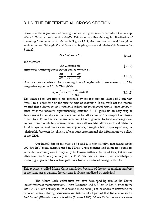
3.1.6. THE DIFFERENTIAL CROSS SECTIONBecause of the importance of the angle of scattering we need to introduce the concept of the differential cross section d σ/d Ω. This term describes the angular distribution of scattering from an atom. As shown in Figure 3.1.3, electrons are scattered through an angle θ into a solid angle Ω and there is a simple geometrical relationship between the θ and Ω)cos 1(2θ−π=Ω [3.1.8]and thereforeθθπ=Ωd d sin 2 [3.1.9] differential scattering cross section can be written asθσθπ=Ωσd d d d sin 21 [3.1.10] Now, we can calculate σ for scattering into all angles which are greater than θ by integrating equation 3.1.10. This yields∫∫ππθθθΩσπ=σ=σ00sin 2d d d d [3.1.11] The limits of the integration are governed by the fact that the values of θ can vary from 0 to π, depending on the specific type of scattering. If we work out the integral we find that σ decreases as θ increases (which makes physical sense). Since d σ/d Ω is often what we measure experimentally, equation 3.1.11 gives us an easy way to determine σ for an atom in the specimen: σ for all values of θ is simply the integral from 0 to π. From this we can use equation 3.1.4 to give us the total scattering cross section from the whole specimen, which we will see later allows us to calculate the TEM image contrast. So we can now appreciate, through a few simple equations, the relationship between the physics of electron scattering and the information we collect in the TEM.Our knowledge of the values of σ and h is very sketchy, particularly at the 100-400 keV beam energies used in TEMs. Cross sections and mean free paths for particular scattering events may only be known within a factor of two, but we can often measure θ very precisely in the TEM. We can combine all our knowledge of scattering to predict the electron paths as a beam is scattered through a thin foil.This process is called Monte Carlo simulation because of the use of random numbers in the computer programs; the outcome is always predicted by statistics!The Monte Carlo calculation was first developed by two of the United States' foremost mathematicians, J. von Neumann and S. Ulam at Los Alamos in the late 1940s. Ulam actually rolled dice and made hand (!) calculations to determine the paths of neutrons through deuterium and tritium which proved that Teller's design for the "Super" (Hbomb) was not feasible (Rhodes 1995). Monte Carlo methods are moreoften used in SEM image calculations (see, e.g., Newbury et al. 1986, Joy 1995), butthey have a role in TEM in determining the expected spatial resolution of microanalysis. Figure 3.1.4 shows two Monte Carlo simulations of electron pathsthrough thin foils.A B Figure 3.1.4. Monte Carlo simulation of the paths followed by 103 100-keV electronsas they pass through thin foils of (A) copper and (B) gold. Notice the increase inscattering with atomic number.。


斯仑贝谢所有测井曲线英文名称解释OCEAN DRILLING PROGRAMACRONYMS USED FOR WIRELINE SCHLUMBERGER TOOLS ACT Aluminum Clay ToolAMS Auxiliary Measurement SondeAPS Accelerator Porosity SondeARI Azimuthal Resistivity ImagerASI Array Sonic ImagerBGKT Vertical Seismic Profile ToolBHC Borehole Compensated Sonic ToolBHTV Borehole TeleviewerCBL Casing Bond LogCNT Compensated Neutron ToolDIT Dual Induction ToolDLL Dual LaterologDSI Dipole Sonic ImagerFMS Formation MicroScannerGHMT Geologic High Resolution Magnetic ToolGPIT General Purpose Inclinometer ToolGR Natural Gamma RayGST Induced Gamma Ray Spectrometry ToolHLDS Hostile Environment Lithodensity SondeHLDT Hostile Environment Lithodensity ToolHNGS Hostile Environment Gamma Ray SondeLDT Lithodensity ToolLSS Long Spacing Sonic ToolMCD Mechanical Caliper DeviceNGT Natural Gamma Ray Spectrometry ToolNMRT Nuclear Resonance Magnetic ToolQSST Inline Checkshot ToolSDT Digital Sonic ToolSGT Scintillation Gamma Ray ToolSUMT Susceptibility Magnetic ToolUBI Ultrasonic Borehole ImagerVSI Vertical Seismic ImagerWST Well Seismic ToolWST-3 3-Components Well Seismic ToolOCEAN DRILLING PROGRAMACRONYMS USED FOR LWD SCHLUMBERGER TOOLSADN Azimuthal Density-NeutronCDN Compensated Density-NeutronCDR Compensated Dual ResistivityISONIC Ideal Sonic-While-DrillingNMR Nuclear Magnetic ResonanceRAB Resistivity-at-the-BitOCEAN DRILLING PROGRAMACRONYMS USED FOR NON-SCHLUMBERGER SPECIALTY TOOLSMCS Multichannel Sonic ToolMGT Multisensor Gamma ToolSST Shear Sonic ToolTAP Temperature-Acceleration-Pressure ToolTLT Temperature Logging ToolOCEAN DRILLING PROGRAMACRONYMS AND UNITS USED FOR WIRELINE SCHLUMBERGER LOGSAFEC APS Far Detector Counts (cps)ANEC APS Near Detector Counts (cps)AX Acceleration X Axis (ft/s2)AY Acceleration Y Axis (ft/s2)AZ Acceleration Z Axis (ft/s2)AZIM Constant Azimuth for Deviation Correction (deg)APLC APS Near/Array Limestone Porosity Corrected (%)C1 FMS Caliper 1 (in)C2 FMS Caliper 2 (in)CALI Caliper (in)CFEC Corrected Far Epithermal Counts (cps)CFTC Corrected Far Thermal Counts (cps)CGR Computed (Th+K) Gamma Ray (API units)CHR2 Peak Coherence, Receiver Array, Upper DipoleCHRP Compressional Peak Coherence, Receiver Array, P&SCHRS Shear Peak Coherence, Receiver Array, P&SCHTP Compressional Peak Coherence, Transmitter Array, P&SCHTS Shear Peak Coherence, Transmitter Array, P&SCNEC Corrected Near Epithermal Counts (cps)CNTC Corrected Near Thermal Counts (cps)CS Cable Speed (m/hr)CVEL Compressional Velocity (km/s)DATN Discriminated Attenuation (db/m)DBI Discriminated Bond IndexDEVI Hole Deviation (degrees)DF Drilling Force (lbf)DIFF Difference Between MEAN and MEDIAN in Delta-Time Proc. (microsec/ft) DRH HLDS Bulk Density Correction (g/cm3)DRHO Bulk Density Correction (g/cm3)DT Short Spacing Delta-Time (10'-8' spacing; microsec/ft)DT1 Delta-Time Shear, Lower Dipole (microsec/ft)DT2 Delta-Time Shear, Upper Dipole (microsec/ft)DT4P Delta- Time Compressional, P&S (microsec/ft)DT4S Delta- Time Shear, P&S (microsec/ft))DT1R Delta- Time Shear, Receiver Array, Lower Dipole (microsec/ft)DT2R Delta- Time Shear, Receiver Array, Upper Dipole (microsec/ft)DT1T Delta-Time Shear, Transmitter Array, Lower Dipole (microsec/ft)DT2T Delta-Time Shear, Transmitter Array, Upper Dipole (microsec/ft)DTCO Delta- Time Compressional (microsec/ft)DTL Long Spacing Delta-Time (12'-10' spacing; microsec/ft)DTLF Long Spacing Delta-Time (12'-10' spacing; microsec/ft)DTLN Short Spacing Delta-Time (10'-8' spacing; microsec/ftDTRP Delta-Time Compressional, Receiver Array, P&S (microsec/ft)DTRS Delta-Time Shear, Receiver Array, P&S (microsec/ft)DTSM Delta-Time Shear (microsec/ft)DTST Delta-Time Stoneley (microsec/ft)DTTP Delta-Time Compressional, Transmitter Array, P&S (microsec/ft)DTTS Delta-Time Shear, Transmitter Array, P&S (microsec/ft)ECGR Environmentally Corrected Gamma Ray (API units)EHGR Environmentally Corrected High Resolution Gamma Ray (API units) ENPH Epithermal Neutron Porosity (%)ENRA Epithermal Neutron RatioETIM Elapsed Time (sec)FINC Magnetic Field Inclination (degrees)FNOR Magnetic Field Total Moment (oersted)FX Magnetic Field on X Axis (oersted)FY Magnetic Field on Y Axis (oersted)FZ Magnetic Field on Z Axis (oersted)GR Natural Gamma Ray (API units)HALC High Res. Near/Array Limestone Porosity Corrected (%)HAZI Hole Azimuth (degrees)HBDC High Res. Bulk Density Correction (g/cm3)HBHK HNGS Borehole Potassium (%)HCFT High Resolution Corrected Far Thermal Counts (cps)HCGR HNGS Computed Gamma Ray (API units)HCNT High Resolution Corrected Near Thermal Counts (cps)HDEB High Res. Enhanced Bulk Density (g/cm3)HDRH High Resolution Density Correction (g/cm3)HFEC High Res. Far Detector Counts (cps)HFK HNGS Formation Potassium (%)HFLC High Res. Near/Far Limestone Porosity Corrected (%)HEGR Environmentally Corrected High Resolution Natural Gamma Ray (API units) HGR High Resolution Natural Gamma Ray (API units)HLCA High Res. Caliper (inHLEF High Res. Long-spaced Photoelectric Effect (barns/e-)HNEC High Res. Near Detector Counts (cps)HNPO High Resolution Enhanced Thermal Nutron Porosity (%)HNRH High Resolution Bulk Density (g/cm3)HPEF High Resolution Photoelectric Effect (barns/e-)HRHO High Resolution Bulk Density (g/cm3)HROM High Res. Corrected Bulk Density (g/cm3)HSGR HNGS Standard (total) Gamma Ray (API units)HSIG High Res. Formation Capture Cross Section (capture units) HSTO High Res. Computed Standoff (in)HTHO HNGS Thorium (ppm)HTNP High Resolution Thermal Neutron Porosity (%)HURA HNGS Uranium (ppm)IDPH Phasor Deep Induction (ohmm)IIR Iron Indicator Ratio [CFE/(CCA+CSI)]ILD Deep Resistivity (ohmm)ILM Medium Resistivity (ohmm)IMPH Phasor Medium Induction (ohmm)ITT Integrated Transit Time (s)LCAL HLDS Caliper (in)LIR Lithology Indicator Ratio [CSI/(CCA+CSI)]LLD Laterolog Deep (ohmm)LLS Laterolog Shallow (ohmm)LTT1 Transit Time (10'; microsec)LTT2 Transit Time (8'; microsec)LTT3 Transit Time (12'; microsec)LTT4 Transit Time (10'; microsec)MAGB Earth's Magnetic Field (nTes)MAGC Earth Conductivity (ppm)MAGS Magnetic Susceptibility (ppm)MEDIAN Median Delta-T Recomputed (microsec/ft)MEAN Mean Delta-T Recomputed (microsec/ft)NATN Near Pseudo-Attenuation (db/m)NMST Magnetometer Temperature (degC)NMSV Magnetometer Signal Level (V)NPHI Neutron Porosity (%)NRHB LDS Bulk Density (g/cm3)P1AZ Pad 1 Azimuth (degrees)PEF Photoelectric Effect (barns/e-)PEFL LDS Long-spaced Photoelectric Effect (barns/e-)PIR Porosity Indicator Ratio [CHY/(CCA+CSI)]POTA Potassium (%)RB Pad 1 Relative Bearing (degrees)RHL LDS Long-spaced Bulk Density (g/cm3)RHOB Bulk Density (g/cm3)RHOM HLDS Corrected Bulk Density (g/cm3)RMGS Low Resolution Susceptibility (ppm)SFLU Spherically Focused Log (ohmm)SGR Total Gamma Ray (API units)SIGF APS Formation Capture Cross Section (capture units)SP Spontaneous Potential (mV)STOF APS Computed Standoff (in)SURT Receiver Coil Temperature (degC)SVEL Shear Velocity (km/s)SXRT NMRS differential Temperature (degC)TENS Tension (lb)THOR Thorium (ppm)TNRA Thermal Neutron RatioTT1 Transit Time (10' spacing; microsec)TT2 Transit Time (8' spacing; microsec)TT3 Transit Time (12' spacing; microsec)TT4 Transit Time (10' spacing; microsec)URAN Uranium (ppm)V4P Compressional Velocity, from DT4P (P&S; km/s)V4S Shear Velocity, from DT4S (P&S; km/s)VELP Compressional Velocity (processed from waveforms; km/s)VELS Shear Velocity (processed from waveforms; km/s)VP1 Compressional Velocity, from DT, DTLN, or MEAN (km/s)VP2 Compressional Velocity, from DTL, DTLF, or MEDIAN (km/s)VCO Compressional Velocity, from DTCO (km/s)VS Shear Velocity, from DTSM (km/s)VST Stonely Velocity, from DTST km/s)VS1 Shear Velocity, from DT1 (Lower Dipole; km/s)VS2 Shear Velocity, from DT2 (Upper Dipole; km/s)VRP Compressional Velocity, from DTRP (Receiver Array, P&S; km/s) VRS Shear Velocity, from DTRS (Receiver Array, P&S; km/s)VS1R Shear Velocity, from DT1R (Receiver Array, Lower Dipole; km/s) VS2R Shear Velocity, from DT2R (Receiver Array, Upper Dipole; km/s) VS1T Shear Velocity, from DT1T (Transmitter Array, Lower Dipole; km/s) VS2T Shear Velocity, from DT2T (Transmitter Array, Upper Dipole; km/s) VTP Compressional Velocity, from DTTP (Transmitter Array, P&S; km/s) VTS Shear Velocity, from DTTS (Transmitter Array, P&S; km/s)#POINTS Number of Transmitter-Receiver Pairs Used in Sonic Processing W1NG NGT Window 1 counts (cps)W2NG NGT Window 2 counts (cps)W3NG NGT Window 3 counts (cps)W4NG NGT Window 4 counts (cps)W5NG NGT Window 5 counts (cps)OCEAN DRILLING PROGRAMACRONYMS AND UNITS USED FOR LWD SCHLUMBERGER LOGSAT1F Attenuation Resistivity (1 ft resolution; ohmm)AT3F Attenuation Resistivity (3 ft resolution; ohmm)AT4F Attenuation Resistivity (4 ft resolution; ohmm)AT5F Attenuation Resistivity (5 ft resolution; ohmm)ATR Attenuation Resistivity (deep; ohmm)BFV Bound Fluid Volume (%)B1TM RAB Shallow Resistivity Time after Bit (s)B2TM RAB Medium Resistivity Time after Bit (s)B3TM RAB Deep Resistivity Time after Bit (s)BDAV Deep Resistivity Average (ohmm)BMAV Medium Resistivity Average (ohmm)BSAV Shallow Resistivity Average (ohmm)CGR Computed (Th+K) Gamma Ray (API units)DCAL Differential Caliper (in)DROR Correction for CDN rotational density (g/cm3).DRRT Correction for ADN rotational density (g/cm3).DTAB AND or CDN Density Time after Bit (hr)FFV Free Fluid Volume (%)GR Gamma Ray (API Units)GR7 Sum Gamma Ray Windows GRW7+GRW8+GRW9-Equivalent to Wireline NGT window 5 (cps) GRW3 Gamma Ray Window 3 counts (cps)-Equivalent to Wireline NGT window 1GRW4 Gamma Ray Window 4 counts (cps)-Equivalent to Wireline NGT window 2GRW5 Gamma Ray Window 5 counts (cps)-Equivalent to Wireline NGT window 3GRW6 Gamma Ray Window 6 counts (cps)-Equivalent to Wireline NGT window 4GRW7 Gamma Ray Window 7 counts (cps)GRW8 Gamma Ray Window 8 counts (cps)GRW9 Gamma Ray Window 9 counts (cps)GTIM CDR Gamma Ray Time after Bit (s)GRTK RAB Gamma Ray Time after Bit (s)HEF1 Far He Bank 1 counts (cps)HEF2 Far He Bank 2 counts (cps)HEF3 Far He Bank 3 counts (cps)HEF4 Far He Bank 4 counts (cps)HEN1 Near He Bank 1 counts (cps)HEN2 Near He Bank 2 counts (cps)HEN3 Near He Bank 3 counts (cps)HEN4 Near He Bank 4 counts (cps)MRP Magnetic Resonance PorosityNTAB ADN or CDN Neutron Time after Bit (hr)PEF Photoelectric Effect (barns/e-)POTA Potassium (%) ROPE Rate of Penetration (ft/hr)PS1F Phase Shift Resistivity (1 ft resolution; ohmm)PS2F Phase Shift Resistivity (2 ft resolution; ohmm)PS3F Phase Shift Resistivity (3 ft resolution; ohmm)PS5F Phase Shift Resistivity (5 ft resolution; ohmm)PSR Phase Shift Resistivity (shallow; ohmm)RBIT Bit Resistivity (ohmm)RBTM RAB Resistivity Time After Bit (s)RING Ring Resistivity (ohmm)ROMT Max. Density Total (g/cm3) from rotational processing ROP Rate of Penetration (m/hr)ROP1 Rate of Penetration, average over last 1 ft (m/hr).ROP5 Rate of Penetration, average over last 5 ft (m/hr)ROPE Rate of Penetration, averaged over last 5 ft (ft/hr)RPM RAB Tool Rotation Speed (rpm)RTIM CDR or RAB Resistivity Time after Bit (hr)SGR Total Gamma Ray (API units)T2 T2 Distribution (%)T2LM T2 Logarithmic Mean (ms)THOR Thorium (ppm)TNPH Thermal Neutron Porosity (%)TNRA Thermal RatioURAN Uranium (ppm)OCEAN DRILLING PROGRAMADDITIONAL ACRONYMS AND UNITS(PROCESSED LOGS FROM GEOCHEMICAL TOOL STRING)AL2O3 Computed Al2O3 (dry weight %)AL2O3MIN Computed Al2O3 Standard Deviation (dry weight %) AL2O3MAX Computed Al2O3 Standard Deviation (dry weight %) CAO Computed CaO (dry weight %)CAOMIN Computed CaO Standard Deviation (dry weight %) CAOMAX Computed CaO Standard Deviation (dry weight %) CACO3 Computed CaCO3 (dry weight %)CACO3MIN Computed CaCO3 Standard Deviation (dry weight %) CACO3MAX Computed CaCO3 Standard Deviation (dry weight %) CCA Calcium Yield (decimal fraction)CCHL Chlorine Yield (decimal fraction)CFE Iron Yield (decimal fraction)CGD Gadolinium Yield (decimal fraction)CHY Hydrogen Yield (decimal fraction)CK Potassium Yield (decimal fraction)CSI Silicon Yield (decimal fraction)CSIG Capture Cross Section (capture units)CSUL Sulfur Yield (decimal fraction)CTB Background Yield (decimal fraction)CTI Titanium Yield (decimal fraction)FACT Quality Control CurveFEO Computed FeO (dry weight %)FEOMIN Computed FeO Standard Deviation (dry weight %) FEOMAX Computed FeO Standard Deviation (dry weight %) FEO* Computed FeO* (dry weight %)FEO*MIN Computed FeO* Standard Deviation (dry weight %) FEO*MAX Computed FeO* Standard Deviation (dry weight %) FE2O3 Computed Fe2O3 (dry weight %)FE2O3MIN Computed Fe2O3 Standard Deviation (dry weight %) FE2O3MAX Computed Fe2O3 Standard Deviation (dry weight %) GD Computed Gadolinium (dry weight %)GDMIN Computed Gadolinium Standard Deviation (dry weight %) GDMAX Computed Gadolinium Standard Deviation (dry weight %) K2O Computed K2O (dry weight %)K2OMIN Computed K2O Standard Deviation (dry weight %)K2OMAX Computed K2O Standard Deviation (dry weight %) MGO Computed MgO (dry weight %)MGOMIN Computed MgO Standard Deviation (dry weight %) MGOMAX Computed MgO Standard Deviation (dry weight %)S Computed Sulfur (dry weight %)SMIN Computed Sulfur Standard Deviation (dry weight %) SMAX Computed Sulfur Standard Deviation (dry weight %)SIO2 Computed SiO2 (dry weight %)SIO2MIN Computed SiO2 Standard Deviation (dry weight %) SIO2MAX Computed SiO2 Standard Deviation (dry weight %) THORMIN Computed Thorium Standard Deviation (ppm) THORMAX Computed Thorium Standard Deviation (ppm)TIO2 Computed TiO2 (dry weight %)TIO2MIN Computed TiO2 Standard Deviation (dry weight %) TIO2MAX Computed TiO2 Standard Deviation (dry weight %) URANMIN Computed Uranium Standard Deviation (ppm) URANMAX Computed Uranium Standard Deviation (ppm) VARCA Variable CaCO3/CaO calcium carbonate/oxide factor。

非线性科学,球形闪电和一般的三维非线性波的电磁孤子模型张一方(云南大学物理系,昆明650091)摘要:非线性科学是当代科学发展的主要前沿之一。
由此得到的地震震级-周期公式预报的地震,不断被证实。
非线性引力波的预言也被证实。
球形闪电是大自然中一个未解之谜。
由非线性电磁场、非线性光学、一般的非线性电磁相互作用及其他非线性方程可以定量导出三维非线性波的电磁孤子模型,进而由此推测球形闪电应该是电磁孤子的特例。
关键词:非线性;球形闪电;电磁场;孤子;波中图分类号:P315.02文献标志码:A文章编号:1673-2928(2021)02-0090-05收稿日期:2020-9-15基金项目:国家自然科学基金项目(11664044)。
作者简介:张一方(1947-),男,云南人,教授,主要研究理论物理和交叉科学。
DOI:10.19329/ki.1673-2928.2021.02.0222021年3月第20卷第2期(总第110期)安阳工学院学报Journal of Anyang Institute of TechnologyMar,2021Vol.20No.2(Gen.No.110)非线性科学是当代科学发展的主要前沿之一。
众所周知,非线性科学有3个研究热点:混沌、孤子和分形。
1988年笔者提出一种粒子的分形模型,并推广分数维为复数维[1]。
对此《人民日报海外版》2002年4月29日第6版和哈尔滨工业大学出版社2004年出版的《探索未知世界》物理篇中68-69页都做过报道。
近年,笔者进一步展开了更深入的研究[2-3]。
本文讨论了某些非线性理论,并基于一般的非线性电磁场及其非线性方程定量导出三维非线性波的电磁孤子模型,由此推测球形闪电应该是电磁孤子的特例。
1某些非线性理论基于非线性流体力学方程等,可以导出笔者1989年提出的地震震级-周期公式[4-9]:T =T 010-b (M 0-M )(1)基于此可以在一定的时空范围对大地震做出定量预言。

块交织及解交织实验报告引言本实验旨在研究块交织(block interleaving)和解交织(deinterleaving)技术在通信领域的应用。
通过对块交织和解交织过程的详细分析和实验验证,探讨这些技术在提高通信系统性能方面的价值。
1. 块交织技术1.1 块交织概念块交织是一种将输入数据按照块的形式进行重新排列的技术。
其目的是增加输入数据之间的冗余度,从而提高数据在信道中传输的容错性。
具体而言,块交织将输入数据分成若干个块,然后逐个交织,形成输出块。
输出块中的数据通过重排列,使得相邻输入数据在输出数据中相隔较远,减小了受到信道连续错误影响的可能性。
1.2 块交织算法常见的块交织算法包括行交织(row interleaving)和列交织(column interleaving)。
行交织算法将输入数据按照行的方式进行交织,即将一行中的数据依次填入输出块中,并逐行进行。
列交织算法则是将输入数据按照列的方式进行填入输出块。
两种算法各有优劣,根据具体信道的特点和通信系统要求进行选择。
1.3 块交织实验设计本实验选择了行交织算法作为研究对象,以便于直观展示块交织的过程。
实验中使用了信道模型进行模拟,通过设置不同的块大小和交织次数,观察输出数据的特性变化。
具体实验步骤如下: 1. 确定输入数据大小和块大小,设置交织次数。
2. 将输入数据按照块大小进行分块。
3. 根据行交织算法,逐个交织输入数据块,形成输出数据块。
4. 进行指定的交织次数,直到得到最终输出数据。
2.1 块大小对交织效果的影响在实验中,我们设置了不同的块大小进行测试,并比较了其交织效果。
结果显示,随着块大小的增加,输出数据的冗余度提高,即相邻输入数据在输出中的间隔增大。
这表明较大的块大小能够提高交织效果,增加数据传输的容错性。
2.2 交织次数对交织效果的影响我们还进行了交织次数的测试,观察其对交织效果的影响。
实验中,我们固定块大小,逐步增加交织次数进行测试。
Phase diagramHello everybody, welcome to my class. Today, we will talk about phase diagram and Gibbs phase rule, as well as how to calculate the corresponding proportion of liquid phase and solid phase.译文:大家好,欢迎来到我的课程。
今天,我们将讨论相图,吉布斯相律,以及如何计算液相和固相的相对含量。
First of all, let’s introduce the definition of phase. Phase is defined as a homogeneous part or aggregation of material. This homogenous part is distinguished from another part due to difference in structure, composition, or both. The different structures form an interface to difference in structure and composition. (这里要注意相的概念,相是指在结构和组成方面与其它部分不同的均匀体。
)译文:我们首先学习相的定义。
相是指在一种材料中,结构、组成,或两者同时不同于其他部分的均匀体或聚集体部分。
不同部分间形成界面,也就是相与相之间的分界面。
Some solid materials have the capability of changing their crystal structure under the varying conditions of pressure and temperature, causing an ability of phase-change.译文:一些固体材料随着压力和温度条件的改变而发生结晶结构变化,具有相变的能力。
a r X i v :h e p -p h /0307005v 2 15 J u l 2003YITP-SB-03-24INLO-PUB-08/03Differential Cross Sections for Higgs ProductionV.RavindranHarish-Chandra Research Institute,Chhatnag Road,Jhunsi,Allahabad,211019,India.J.SmithC.N.Yang Institute for Theoretical Physics,State University of New York at Stony Brook,New York 11794-3840,USA.W.L.van Neerven Instituut-Lorentz University of Leiden,PO Box 9506,2300RA Leiden,The Netherlands.AbstractWe review recent theoretical progress in evaluating higher order QCD corrections to Higgs boson differential distributions at hadron-hadron colliders.1IntroductionThe origin of the spontaneous symmetry breaking mechanism (ssbm)in particle physics is still unknown.In the Standard Model (SM)[1]a vacuum expectation value (vev)v =246GeV is given to components of a complex scalar doublet.Three of these fields generate mass terms for the W ±and Z bosons.The remaining scalar is called the Higgs [2]and has not been observed.The present lower limit for m H from the LEP experiments [3]is 114GeV/c 2.In the SM the interaction vertices with scalar fields are expressed in terms of v and m H .Extensions of the standard model to incorporate supersymmetry contain several Higgs particles,both scalar and pseudoscalar [4].In the minimal supersymmetric extension of the Standard Model (MSSM),there are two Higgs doublets,so it is called the Two-Higgs-Doublet Model (2HDM).After implementing the ssbm there are five Higgs bosons usually denoted by h,H ,(CP even),A (CP odd)and H ±.At tree level their couplings and masses depend on two parameters,m A and the ratio of two vevs,parametrized by tan β=v 2/v 1.Since no Higgs particle has been found the region m A <92GeV/c 2and 0.5<tan β<2.4is experimentally excluded [5].For recent reviews on the theoretical status of total Higgs boson cross sections see [6].Let us denote the neutral bosons h,H,A collectively by B.It is possible that a B will be detected at the Fermilab Tevatron p −¯p collider (√S =14TeV).If no B is found then thessbm must be realized in a different way,possibly via dynamical interactions between the gauge bosons.In parallel with the ongoing experimental effort higher order quantum chromodynamic (QCD)corrections to B production differential distributions are needed.The leading order (LO)partonic reactions were calculated quite a long time ago and the next-to-leading order (NLO)corrections to these distributions only recently.Note that the detection of the B via its decay products depends on m B .The present mass limits allow the decays B →γγ,B →b ¯b andB →W W ∗,ZZ ∗where W ∗and Z ∗are virtual vector bosons,which are detected as leptons and/or hadrons (jets).As m B increases other decay channels (for example B →W +W −,ZZ ,B →t ¯t),open up requiring different experimental triggers.Higher order QCD corrections to these decay rates have also been calculated but will not be discussed here.2Higgs differential distributionsFor inclusive B-production one calculates the differential cross section in the B transverse mo-mentum (p T )and its rapidity (y ),which are functions of m B ,the partonic momentum fractions x 1,x 2in the hadron beams,and the partonic cm energy √x 1x 2S .All other final state particles are integrated over.In contrast exclusive B-production retains the information on these other particles.In the SM the H couples to the gluons via quark loops with the ¯q q H vertex pro-portional to m q ,so the t-quark loop is the most important.In the 2HDM the gg A amplitude with quark loops depends on both the masses of the quarks and β.In LO the g +g →H crosssection (order α2s )containing the top-quark triangle graph,was computed in [7].However here p T =0,so we need a two-to-two body partonic process to produce a Higgs with a finite p T .Note that these are NLO processes with respect to the total B production cross section and oforder α3s .At small x the gluon density g (x,Q 2)>q i (x,Q 2)>¯q i (x,Q 2),(q i stand for u,d,s,c,b,t quarks)so we expect that,in order of importance,the dominant production channels areg +g →g +B,g +q i (¯q i )→q i (¯q i )+B,q i +¯q i→g +B.(2.1)These are the LO order Born reactions for Higgs p T and y distributions.The correspondingFeynman diagrams contain heavy quark box graphs.The B differential distributions for the reactions in Eq.(2.1)were computed for B=H in [8]and for B=A in [9].The total cross section,which also contains the virtual QCD corrections to the gg B top-quark triangle,was calculated in [10],[11]and [12].The expressions in [12]for the two-loop graphs with finite m t and m B are very complicated.Furthermore also the two-to-three body reactions (e.g.g +g →g +g +B involving pentagon loops)have been computed in [13]using helicity methods.From these results it isclear that it will be very difficult to obtain the NLO (order α4s )corrections to the B differential distributions as functions of both m t and m B .Fortunately one can simplify the calculations if one takes the limit m t →∞.In this case the Feynman graphs are obtained from an effective Lagrangian describing the direct Bgg coupling.An analysis in [14]in NLO reveals that the error introduced by taking the m t →∞limit is less than about 5%provided m B ≤2m t .The two-to-three body processes were computed with the effective Lagrangian approach for the B in [15]and [16]respectively using helicity methods.The one-loop corrections to the two-to-two body reactions above were computed for the H in [17]and the A in [9].These NLO matrix elements (order α4s )were used to compute the p T and y distributions of the H in [18],[19],[20],[21]and the A in [22].For ways to differentiate between production of H and A see [23]and references therein.In the large m t limit the Feynman rules(see e.g.[15])for scalar H production can be derived from the following effective Lagrangian densityL H eff=G HΦH(x)O(x)with O(x)=−18ǫµνλσGµνa(x)Gλσa(x),O2(x)=−1m2t ,˜GA=− a s(µ2r)C F 3m2t +··· G A,(2.4) where a s(µ2r)is defined bya s(µ2r)=αs(µ2r)m2B,f(τ)=arcsin21τ,forτ≥1,f(τ)=−11−τ1−τ+πi 2forτ<1,(2.6)whereβdenotes the mixing angle in the2HDM.In the large m t-limit we havelim τ→∞F H(τ)=2τcotβ.(2.7)The coefficient functions C B originate from the corrections to the top-quark triangle graph pro-vided one takes the limit m t→∞.The coefficient functions were computed up to orderα2s in[14],[24]for the H and in[25]for the A.The answer depends upon a(5)s,the running coupling in thefive-flavour number scheme,and we only need thefirst order termsC H a s(µ2r),µ2rm2t =1.(2.8) The last result holds to all orders because of the Adler-Bardeen theorem[26].3Numerical results at moderate p TThe hadronic cross section dσfor H1(P1)+H2(P2)→B(−P5)+X is obtained from the partonic cross sections dσab for the reactions in Eq.(2.1)and their NLO corrections[for example g(p1)+ g(p2)→g(−p3)+g(−p4)+B(−p5)]usingS2d2σH1H2x1 1x2,min dx2d t d u(s,t,u,m2B,µ2).(3.9)Here f H a(x,µ2)is the parton density for parton a in hadron H at factorization/renormalization scaleµand the hadronic kinematical variables are defined byS=(P1+P2)2,T=(P1+P5)2,U=(P2+P5)2.(3.10) The latter two invariants can be expressed in terms of the p T and y variables byT=m2B−√p2T+m2B cosh y+√p2T+m2B sinh y,U=m2B−√p2T+m2B cosh y−√p2T+m2B sinh y.(3.11) In the case parton p1emerges from hadron H1(P1)and parton p2emerges from hadron H2(P2) we can establish the following relationsp1=x1P1,p2=x2P2,s=x1x2S,t=x1(T−m2B)+m2B,u=x2(U−m2B)+m2B,x1,min=−U x1S+U−m2B.(3.12)Since the differential cross section contains terms in m B/p T ln i(m B/p T),(i=1,2,3)which are not integrable at p T=0,we cannot integrate over p T down to p T=0tofind the y-distribution. However we can integrate over y tofind the p T-distribution,valid over a range in p T where there are no large logarithms,(say p T>30GeV/c),dσH1H2d p T d y(S,p2T,y,m2B),(3.13)Figure1:The differential cross section dσ/dp T integrated over the whole rapidity range(see Eq.(3.13))with m H=120GeV/c2andµ2=m2H+p2T.The LO plots are presented for thesubprocesses gg(long-dashed line),q(¯q)g(dot-dashed line)and100×(q¯q)(dotted line)using the parton density set MRST98(lo05a.dat).with afixed y max.The calculation of the NLO B differential distributions requires the virtual corrections to the reactions in Eq.(2.1)and the NLO two-to-three body reactions(orderα4s).Hence one needs a regularization scheme,and renormalization and mass factorization(whichintroduces the scalesµr andµf respectively).The presence of theγ5matrix in the pseudoscalar contributions makes everything even more complicated and we refer to[22]for details.In[18]helicity amplitudes were used and the fully exclusive two-to-three body reactions were calculatednumerically.Very few formulae were presented.In[19]the cancellations of the UV and IR singularities were done algebraically leading to the H inclusive distributions.Many analyticalresults were given but the two-to-three body matrix elements were too long to publish.In[20], [21]helicity amplitudes were used for the H inclusive calculation and complete analytical resultswere provided.The numerical results from these three papers have been compared against eachother and they agree.We put n f=5in a s(µ2r),σab and f H a(x,µ2)in Eq.(3.9).For simplicityµr=µf=µand wetakeµ2=m2H+p2T for our plots.Further we have used the parton density sets MRST98[27], MRST99[28],GRV98[29],CTEQ4[30]and CTEQ5[31].We want to emphasize that the magnitudes of the cross sections are extremely sensitive tothe choice of the renormalization scale because the effective coupling constants in Eq.(2.4)are proportional toαs(µr),which implies that dσLO∼α3s and dσNLO∼α4s.However the slopes of the differential distributions are less sensitive to the scale choice if they are only plotted over alimited range.For the computation of the gg B effective coupling constants in Eq.(2.4)we take m t=173.4GeV/c2and G F=1.16639GeV−2=4541.68pb.Here we will only give results for H production at the ck of space limits us to showing only p T-distributions.The LO and NLO p T differential cross sections in Eq.(3.13)with m H=120GeV/c2are shown in Figs.1 and2respectively.The MRST98parton densities[27]were used for these plots.We note thatFigure2:Same as Fig.1in NLO except for100∗abs(q¯q)(dotted line)and the additional subprocess100×abs(qq)(short-dashed line)using the parton density set MRST98(ft08a.dat). the NLO results from the q(¯q)g and qq channels are negative at small p T so we have plotted their absolute values multiplied by100.Clearly the gg reaction dominates.The q(¯q)g reaction is lower by a factor of aboutfive.Regarding the corresponding distributions for A-production they have the same shape depen-dence in LO and differ slightly in NLO.Therefore the only difference is in the overall couplings in Eq.(2.4).In particular if tanβ=1then dσA/dσH=9/4for all values of m H and m A in LO. There are small differences from9/4in NLO.Plots are presented in[22].We now show the scale dependence of the distributions.We have chosen the scale factors µ=2µ0,µ=µ0andµ=µ0/2withµ20=m2H+p2T and plot in Fig.3the quantityN p T,µdσ(p T,µ0)/dp T(3.14)in the range0.1<µ/µ0<10atfixed values of p T=30,70and100GeV/c.The upper set of curves at smallµ/µ0are for LO and the lower set are for NLO.Notice that the NLO plots at 70and100are extremely close to each other and it is hard to distinguish between them.One sees that the slopes of the LO curves are larger that the slopes of the NLO curves.This is an indication that there is a small improvement in stability in NLO,which was expected.However there is no sign of aflattening or an optimum in either of these curves which implies that one will have to calculate the differential cross sections in NNLO tofind a better stability under scale variations.Next we show the mass dependence of the NLO result in Fig.4using the MRST99parton densities.The differential distribution drops by a factor of two as m H increases from120to180 GeV/c2.There are two other uncertainties which affect the predictive power of the theoretical cross sections.Thefirst one concerns the rate of convergence of the perturbation series which isFigure3:The quantity N(p T,µ/µ0)(see Eq.(3.14)),plotted in the range0.1<µ/µ0<10 atfixed values of p T with m H=120GeV/c2andµ20=m2H+p2T using the MRST98parton density sets.The results are shown for p T=30GeV/c(solid line),p T=70GeV/c(dashed line),p T=100GeV/c(dot-dashed line).The upper three curves on the left hand side are the LO results whereas the lower three curves refer to NLO.indicated by the K-factor defined byK=dσNLOdσMRST ,R GRV=dσGRVFigure4:The mass dependence of dσNLO/dp T(see Eq.(3.13))using the set MRST99(cor01.dat) withµ2=m2H+p2T for Higgs masses m H=120GeV/c2(solid line),m H=160GeV/c2(dashed line)and m H=200GeV/c2(dot-dashed line).contributions which are regular at s4=(p3+p4)2=0and adding the pieces from the virtual contributions.These two contributions constitute the S+V gluon approximation.To study its validity we show in Fig.5the ratiodσS+VR S+V=S/2=7×103GeV/c.Therefore it is rather fortuitous that the approximation works so well for p T>100GeV/c where one obtains R S+V<1.2.The S+V gluon approximation overestimates the exact NLO result but the difference de-creases when the p T increases.In particular for p T>200GeV/c the S+V approximation is good enough so that resummation techniques could be used to give a better estimate of the Higgs boson p T distribution corrected up to all orders in perturbation theory.Note that the boundary of phase space is also approached when m B increases atfixed p T,but,according to the results in Fig.5,the S+V approximation does not improve.In[21]it was noted that in-creasing m B makes the terms in ln(m B/p T)larger atfixed p T.So the range in p T where the small p T-logarithms dominate increases with increasing m B.This leads us to the next topic.Figure5:The ratio R S+V in Eq.(4.17)for the p T distributions using the set MRST99(cor01.dat) withµ2=m2H+p2T,min and various Higgs masses given by m H=120GeV/c2(solid line), m H=160GeV/c2(dashed line)and m H=200GeV/c2(dot-dashed line).5Numerical results at small p TWe noted previously that there are terms in m B/p T ln i(m B/p T)which are dominant in the small p T region.In this region the double differential cross section can be expanded as followsdσs m2B2π m C mn ln m2BFigure6:The Higgs p T spectrum compared to the small-p T limit formula(see Eq.(5.18))at both LO and NLO with CTEQ5L and CTEQ5M1parton densities respectively.All curves are calculated for y=0in the m t=∞effective theory.References[1]S.L.Glashow,Nucl.Phys.22,579(1961);A.Salam,Elementary Particle Theory,NobelSymposium,No.8,ed.N.Svartholm(Stockholm;Almqvist and Wiksell Forlag A.B1968).p.367;S.Weinberg,Phys.Rev.Lett.19,1264(1967).[2]P.W.Higgs,Phys.Lett.12,132(1964);Phys.Rev.Letts.13,508(1964);Phys.Rev.145,1156(1966);F.Englert and R.Brout,Phys.Rev.Lett.13,321(1964);G.S.Guralnik,C.R.Hagen and T.W.Kibble,Phys.Rev.Letts.13,585(1964).[3]R.Barate et al.(ALEPH Collaboration),Phys.Lett.B495,1(2000),hep-ex/001145;M.Acciarri et al.(L3Collaboration),Phys.Lett.B508,225(2001),hep-ex/0012019;P.Abreu et al.(DELPHI Collaboration),Phys.Lett.B499,23(2001),hep-ex/0102036;G.Abbiendi et al.(OPAL Collaboration),Phys.Lett.B499,38(2001),hep-ex/0101014.[4]J.F.Gunion,H.E.Haber,G.L.Kane and S.Dawson,The Higgs Hunter’s Guide,(Addison-Wesley,Reading,M.A.,1990),Erratum ibid.hep/ph-9302272.[5]LEP Collaborations,CERN-EP/2001-055(2001),hep-ex/0107029;LEP Higgs Working Group,hep-ex/0107030;P.Igo-Kemenes,in K.Hagiwara,et al.(Eds),Review of Particle Physics,Phys.Rev.D 66,010001(2002).[6]D.Rainwater,M.Spira and D.Zeppenfeld,hep-ph/0203187;M.Spira,hep-ph/0211145,S.Dawson,hep-ph/0111226.[7]F.Wilczek,Phys.Rev.Lett.39,1304(1977);H.Georgi,S.Glashow,M.Machacek,D.Nanopoulos,Phys.Rev.Lett.40,692(1978);J.Ellis,M.Gaillard,D.Nanopoulos,C.Sachra-jda,Phys.Lett.B83,339(1979);T.Rizzo,Phys.Rev.D22,178(1980).[8]R.K.Ellis,I.Hinchliffe,M.Soldate,J.J.van der Bij,Nucl.Phys.B297,221(1988);U.Baur,E.W.Glover,Nucl.Phys,B339,38(1990);R.P.Kauffman,Phys.Rev.D44,1415(1992);ibidPhys.Rev.D45,1512(1992).[9]C.Kao,Phys.Lett,B328,420(1994),hep-ph/9310206.[10]S.Dawson,Nucl.Phys.B359,283(1991);R.P.Kauffman,W.Schaffer,Phys.Rev.D49,551(1994);S.Dawson,R.P.Kauffman,Phys.Rev.D49,2298(1994).[11]A.Djouadi,M.Spira and P.M.Zerwas,Phys.Lett.B264,440(1991);D.Graudenz,M.Spira,P.M.Zerwas,Phys.Rev.Lett.70,1372(1993);M.Spira,A.Djouadi,D.Graudenz,P.Zerwas,Phys.Lett.B318,347(1993).[12]M.Spira, A.Djouadi, D.Graudenz,P.Zerwas,Nucl.Phys.B453,17(1995),hep-ph/9504378.[13]V.Del Duca,W.Kilgore,C.Oleari,C.Schmidt and D.Zeppenfeld,Phys.Rev.Lett.87,122001(2001),hep-ph/0105129;ibid Nucl.Phys.B616,367(2001),hep-ph/0108030.[14]M.Kr¨a mer,enen and M.Spira,Nucl.Phys.B511,523(1998),hep/ph9611272.[15]S.Dawson,R.P Kauffman,Phys.Rev.Lett.68,2273(1992);R.P.Kauffman,S.V.Desai,D.Risal,Phys.Rev.D55,4005(1997),Erratum ibid.D58,119901(1998),hep-ph/9610541.[16]R.P.Kauffman,S.V.Desai,Phys.Rev.D59,05704(1999),hep-ph/9808286.[17]C.R.Schmidt,Phys.Lett.B413,391(1997),hep-ph/9707448.[18]D.de Florian,M.Grazzini,Z.Kunszt,Phys.Rev.Lett.82,5209(1999),hep-ph/9902483.[19]V.Ravindran,J.Smith,W.L.van Neerven,Nucl.Phys.B634,247(2002),hep-ph/0201114.[20]C.J.Glosser,hep-ph/0201054.[21]C.J.Glosser and C.R.Schmidt,JHEP0212,016(2002),hep-ph/0209248.[22]B.Field,J.Smith,M.E.Tejeda-Yeomans,W.L.van Neerven,Phys.Lett.B551,137(2003),hep-ph/0210369.[23]B.Field,Phys.Rev.D66,114007(2003),hep-ph/0208262.[24]K.G.Chetyrkin, B.A.Kniehl,M.Steinhauser,Phys.Rev.Lett.79,353(1997),hep-ph/9705240.[25]K.G.Chetyrkin,B.A.Kniehl,M.Steinhauser,W.A.Bardeen,Nucl.Phys.B535,3(1998),hep-ph/9807241.[26]S.L.Adler,W.Bardeen,Phys.Rev.182,1517(1969).[27]A.D.Martin,R.G.Roberts,W.J.Stirling and R.S.Thorne,Eur.Phys.J.C4,463(1998),hep-ph/9803445.[28]A.D.Martin,R.G.Roberts,W.J.Stirling and R.S.Thorne,Eur.Phys.J.C14,133(2000),hep-ph/997231.[29]M.Gl¨u ck,E.Reya,A.Vogt,Eur.Phys.J.C5,461(1998),hep-ph/9806404.[30]i et al.,Phys.Rev.D55,1280(1997),hep-ph/9606399.[31]i et al[CTEQ Collaboration]Eur.Phys.J.C12,375(2000),hep-ph/9903282.[32]P.B.Arnold and R.P.Kauffman,Nucl.Phys.B349,381(1991).[33]S.Catani,D.de Florian,M.Grazzini,Nucl.Phys B596,299(2001),hep-ph/0008184.[34]J.C.Collins,D.E.Soper,Nucl.Phys.B193,381(1981)[Erratum-ibid B213,545(1983)];J.C.Collins,D.E.Soper,Nucl.Phys.B197,446(1982);J.C.Collins,D.E.Soper,G.Sterman, Nucl.Phys.B250,199(1985).[35]I.Hinchliffe,S.F.Novaes,Phys.Rev.D38,3475(1988);R.P.Kauffman,Phys.Rev.D44,1415(1991);R.P.Kauffman,Phys.Rev.D45,1512(1992);S.Catani,E.D’Emilio and L.Trentadue,Phys.Lett.B211,335(1988);C.-P.Yuan,Phys.Lett.B283,395(1992)395;C.Balazs and C.-P.Yuan,Phys.Rev.D59,111407(1999),Erratum ibid.D63(2001)059902, ibid.Phys.Lett.B478,192(2000),hep-ph/0001103;C.Balazs,J.Huston and I.Puljak,Phys.Rev.D63,014021,014021(2001);[36]D.de Florian and M.Grazzini,Phys.Rev.Lett.85,4678(2000),hep-ph/0008152;D.deFlorian and M.Grazzini,Nucl.Phys.616,247(2001);hep-ph/0108273.G.Bozzi,S.Catani,D.de Florian and M.Grazzini,Phys.Lett.B564,65(2003).[37]E.L.Berger and J.w.Qiu,Phys.Rev.D6*******(2003)E.L.Berger and J.w.Qiu,hep-ph/0304267.。